Combining the Polarizable Drude Force Field with a Continuum Electrostatic Poisson-Boltzmann Implicit Solvation Model

Abstract

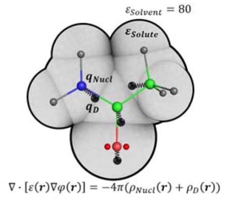
In the present work we have combined the polarizable force field based on the classical Drude oscillator with a continuum Poisson-Boltzmann/Solvent Accessible Surface Area (PB/SASA) model. In practice, the positions of the Drude particles experiencing the solvent reaction field arising from the fixed charges and induced polarization of the solute must be optimized in a self-consistent manner. Here, we parameterized the model to reproduce experimental solvation free energies of a set of small molecules. The model reproduces well experimental solvation free energies of 70 molecules, yielding a root mean square difference of 0.8 kcal/mol versus 2.5 kcal/mol for the CHARMM36 additive force field. The polarization work associated with the solute transfer from the gas-phase to the polar solvent, a term neglected in the framework of additive force fields, was found to make a large contribution to the total solvation free energy, comparable to the polar solute-solvent solvation contribution. The Drude PB/SASA also reproduces well the electronic polarization from the explicit solvent simulations of a small protein, BPTI. Model validation was based on comparisons with the experimental relative binding free energies of 371 single alanine mutations. With the Drude PB/SASA model the root mean square deviation between the predicted and experimental relative binding free energies is 3.35 kcal/mol, lower than 5.11 kcal/mol computed with the CHARMM36 additive force field. Overall, the results indicate that the main limitation of the Drude PB/SASA model is the inability of the SASA term to accurately capture non-polar solvation effects.

Graphical Abstract

The polarizable force field based on the classical Drude oscillator was combined with a continuum Poisson-Boltzmann/Solvent Accessible Surface Area model. In this model the positions of the Drude particles, representing the electronic degrees of freedom, experiencing the solvent reaction field are optimized in a self-consistent manner. The model reproduces well experimental solvation free energies of small molecules, the electronic polarization from an explicit solvent simulation of a small protein, and a large set of experimental protein-protein relative binding free energies.

INTRODUCTION

Aqueous solvent plays a key role in the majority of biological processes, including ligand-protein binding. Upon formation of ligand-protein complexes the environment of the binding site changes significantly by replacement of the polar aqueous solvent by polar and non-polar groups of the ligand. Thus, the ligand-protein binding represents a fine balance between ligand-protein, protein-solvent and ligand-solvent interactions. To model these interactions the most accurate approach is to use models with explicit solvent molecules, which arguably provide the highest level of detail of biomolecular systems and, in principle, allow calculations of precise binding free energies of ligands to targets.^1–3 However, in practice, these simulations remain computationally demanding, especially for problems including de novo protein design, studies of protein-protein interactions and virtual screening of large small molecule databases that require the evaluation of solvation free energies within a few seconds. For this reason a significant amount of efforts has been invested in the development of approximate schemes for treating the solvent implicitly.^4–6 Typically, implicit solvent models represent the solvation energy as a sum of nonpolar and polar contributions.^7,8 The nonpolar contribution is often expressed in terms of the solvent-accessible solute surface area and/or solvent excluded solute volume, while the polar contribution is commonly approximated on the basis of the Poisson equation for continuum dielectric media.^9,10 Numerical solutions to the Poisson equation, or Poisson-Boltzmann (PB) equation when accounting for effect of electrolyte, can provide a very effective approach for treating the influence of electrostatic solvation effects on molecules of arbitrary shape.^11–22

The solvent charge density produces the solvent reaction field acting on the solute atoms, with the largest contribution to this field being produced by the solvent charges and associated polarization directly adjacent to the solute, i.e. near the molecular boundary of the solute.⁸ Thus, results of continuum electrostatics models are especially sensitive to the location of the solute/solvent boundary and its functional form.^9,23–25 In continuum models this boundary is defined on the basis of atomic Born-like radii,²⁵ which normally do not depend on the solute conformation, but may depend on the solute covalent structure. This imposes a restraint on the solvation radii to give accurate results across multiple conformations of the solute. In addition, similar to force field optimization the solvation radii are explicitly parametrized only for a limited set of small compounds, representing the space of all possible molecules. Then these parameters are transferred to larger molecules. This also imposes a restraint that the solvation parameters should work equally well across entire space of molecules, including beyond those for which they are developed. Finally, and probably most importantly, since not all details of the explicit solvent are treated by continuum implicit solvents, such as energetics and directionality of solute-solvent hydrogen bonds, not all aspects of the explicit solvent can be reproduced by implicit solvents. As consequence, the target data and method used to parametrize solvation models and the PB model in particular determine their accuracy and applicability to a particular set of problems.

It was previously shown that the ionic radius of hydration can be approximated as the first peak in the solute-solvent radial distribution function.⁹ As a consequence, the optimal value for ionic radius is not a property of the ion alone but is an empirical quantity depending on the ion as well as on the chemical nature of the surrounding solvent molecules. For example, this is reflected in the difference in solvation free energy between anions and cations in bulk water due to the asymmetric structure of the water molecule.^9,26–29 In principle, the same asymmetry of interactions should be found for polar groups of the solute. Thus, the atomic solvation radii of the solute are defined by the solute and solvent in synergy.³⁰ The solvent radial density function (RDF) around a solute atom shows a complex behavior with several peaks corresponding to different layers of partially structured waters.²⁵ The Poisson model with uniform dielectric media for the solvent and the solute should reproduce the polarization of this non-uniform and granular solvent. For this reason, the solvation radii may not be related directly the solvent radial density distribution function. In addition the Poisson method does not treat all details of the explicit solvent, such as solute-solvent hydrogen bonds, and thus the solvation radii can be regarded as empirical adjustable parameters.

In past parameterizations of continuum electrostatic models either experimental solvation energies^31,32 or explicit solvent simulations^25,33–39 were used to fit solvation parameters. Both methods have advantages and disadvantages. Fitting solvation parameters against explicit solvent simulations relies on the quality of those simulations, which strongly depend on the simulation details and force field parameters (such as charges) of the solute as well as force field parameters of the solvent. On the other hand fitting a solvation model against experimental solvation free energies instantly gives a benchmark of the simulation model against experimental data. Both polar and non-polar terms of the solvation model must be fitted together, since in the experiments it is not possible to separate the polar and non-polar contributions. This is not a disadvantage, since most of the applications of solvation models, such as ligand or protein binding require knowledge of the complete energies and forces acting on solute atoms. However, during optimization of continuum models based on additive force fields, which use fixed-point charges on atoms, the polarization work associated with the transfer of the solute from the gas phase to the bulk solvent is commonly neglected. This may cause problems in the parametrization of continuum solvation models against experimental data, which include the contribution from the polarization. Thus, it is more straightforward in fitting of continuum solvation models to reproduce results of explicit solvent simulations with additive force fields, since these explicit solvent simulations would not include polarization effects. With the Drude force field the polarization work associated with the solute transfer from the gas phase to the solvent can be naturally included in the calculations. Thus, using the Drude polarizable force field, there is no limitation to use experimental solvation free energies as in the case of additive force fields.

In parametrization of the PB model against experimental data, the model must be supplemented with an appropriate non-polar term to reproduce the total solvation energy. Historically one of the first and still one of the most widely-used models is based on the Solvent-Accessible Surface Area (SASA).^40,41 Several studies have pointed out that SASA term is inadequate to reproduce experimental measurements and proposed further to split the non-polar term into a cavity formation contribution and a contribution due to solute-solvent attractive van der Waals interactions.^42–44 We note that an elegant separation of repulsive and attractive forces in LJ potential was originally developed by Weeks, Chandler, and Andersen (WCA) in the context of liquid perturbation theory,⁴⁵ which can be used for calculations of the repulsion-cavity and soft dispersion-VDW contributions by free energy perturbation (FEP) techniques.⁴⁶ For the dispersion vdW contribution to the total free energy Levy et al proposed a continuum solvent van der Waals interaction energy model.⁴⁴ This model is exact for a solute of an arbitrary shape, but needs finding integrals numerically. Later Gallicchio and Levy proposed an analytical approximation for the continuum dispersion term, which employ atomic Born solvation radii of the Generalized Born (GB) model.⁴² Recently, Michael et al proposed a continuum van der Waals model, which uses another form for the analytical approximation of the continuum vdW model.⁴³ The main difference between this model and the analytical approximation of Gallicchio and Levy is that the integral over the solute volume is taken over the 1/r⁶ function, while the model of Gallicchio and Levy makes use of Born solvation radii, which in turn depend on the self GB energies, which are integrals of the 1/r⁴ function (recently proposed flavors of the GB model employ the 1/r⁶ power function^47–49). Since the two functions behave similarly at short distances, the performance of the two models should be comparable. Michael et al also tested the Lazaridis–Karplus (LK) Gaussian model for the cavity and dispersion term. The continuum model and LK model showed a moderate improvement over the surface area term for the performance for a large set of protein stability mutations.

Solvation models in the context of polarizable force fields were developed by several groups. Ponder et al developed a Poisson-Boltzmann solvation model based on the AMOEBA polarizable force field,^50,51 which was demonstrated to accurately reproduce the polarization from explicit solvent simulations. Luo et al adopted a different approach, where atomic partial charges are fitted against quantum mechanics electrostatic potential and solvent reaction field due to solute charges.^52,53 In this method fitting of the ab-initio electrostatic potential is limited to relatively small systems, tractable by quantum mechanics methods. Finally, a self-consistent reaction field (SCRF) methodology in which solution of the Poisson-Boltzmann equation is coupled with determination of the polarization response of the solute was developed for the polarizable force field by Maple et al.⁵⁴

The goal of the present article is to develop a PB continuum electrostatics solvation model combined with the Drude polarizable force field. In this model, the electronic polarization response of the solute is computed in accord with the solvent reaction field produced both by solute charges and solute induced polarization. Since the solvent reaction field depends on the electronic polarization of the solute, the reaction field and polarization must be computed in a self-consistent manner. In the case of the Drude force field, this requires that the positions of the Drude particles representing electronic polarization be optimized by minimizing the total free energy of the solute. Importantly, the implicit solvation forces arising from the continuum dielectric must be reevaluated at each energy minimization iteration. We also present a set of optimized atomic solvation radii for the model based on the SASA approximation. The usefulness and limitation of the current model are discussed in the context of its application to protein-protein relative binding free energy calculations.

METHODS

The Drude Poisson-Boltzmann/Solvent Assessable Surface Area (PB/SASA) solvation model

The solvation free energy of a solute can be defined as the reversible work to transfer the solute from the gas phase to the bulk solvent and can be separated into electrostatic and non-polar contributions via a thermodynamic cycle. In this cycle the solute cavity is first formed in the solvent, then solute-solvent vdW interactions are introduced, and finally solute-solvent electrostatic interactions are switched on:

$$\mathrm{\Delta }{G}_{\text{tot}}=\mathrm{\Delta }{G}_{\text{cavity}}+\mathrm{\Delta }{G}_{\text{vdW}}+\mathrm{\Delta }{G}_{\text{elec}}$$ Eq 1

The non-polar contribution comprised of the cavity and vdW terms is commonly approximated by the Solvent Accessible Surface Area (SASA) model:

$$\mathrm{\Delta }{G}_{\text{np}}=\mathrm{\Delta }{G}_{\text{cavity}}+\mathrm{\Delta }{G}_{\text{vdW}}\approx \alpha ·\text{SASA}+\beta ,$$ Eq 2

where α is a surface tension and β is the non-polar free energy of solvating an infinitely small solute. In attempts to improve the non-polar treatment, the non-polar solvation free energy in Eq 2 was supplemented with a solute volume proportional term.^55,56 In recent work Harris and Pettitt⁵⁷ showed that the solute volume is practically linear in SASA for small molecules, arguing that the additional volume-dependent term alone cannot improve the non-polar solvation model. For this reason, in this work we did not attempt to include the volume-dependent term. Finally, we did not explore possibilities to improve the non-polar treatment by including a continuum van der Waals dispersion model. Indeed, though recent works reported moderate success of such models, in this study we use the classical form of the non-polar term proportional to SASA, widely used in MM/PBSA methods.^58–61 Future efforts will look into the use of more detailed treatments of the nonpolar term in conjunction with the polarizable model.

The electrostatic contribution can be obtained by numerical solution to the Poisson or Poisson-Boltzmann (PB) equation. In the case of additive force fields the PB solvation energy is a difference between the PB energies computed using the high and low dielectric constants for the solvent: $\mathrm{\Delta }{G}_{\text{elec}}=G_{\epsilon =80}^{\text{PB}}-G_{\epsilon =1}^{\text{PB}}$.⁶² Though the same force field charges are used for the low dielectric calculations in the last formula these point charges are normally optimized to reproduce an average polarization in solvent and, thus are not ideal for the gas phase calculations. In the case of the Drude polarizable force field the PB solvation energy can be computed using the electronic structure (ie. charges and induced dipoles based on the positions of the Drude particles) corresponding to the media for which calculations are done. The electrostatic solvation free energy has also an additional contribution due to the work needed to polarize the solute in vacuum from its vacuum polarization to its polarization in solvent. This contribution does not exist by definition when fixed charges additive force fields are used.

Parametrization scheme

Empirical force field calculations were performed with the program CHARMM.⁶³ Additive force field calculations used the CHARMM36 (C36) and CGenFF force field⁶⁴ while the polarizable model calculations used the Drude-2013 protein and nucleic acid force field.^65,66 We note that the CGenFF parameters are identical to the parameters in the CHARMM36 force field for small compounds used to parametrize the CHARMM36 force field for proteins and we will refer to the additive force field as C36 in the remainder of this paper. For this study, due to poor agreement with experiment hydration free energies updated parameters in the Drude force field for imidazole, 4-methylimidazole, methylamine, ethylamine, and propyl-1-amine were used, as described in the Supporting Information.

Data set

To optimize radii and solvent accessible surface area (SASA) parameters, a set of small molecules with known experimental solvation free energies was used.⁶⁷ The data set contains 70 molecules: 19 non-polar, 43 polar and 8 charged molecules (Table S1, Supporting Information). The experimental solvation data were taken from the experimental dataset of hydration free energies from the work of Mobley et al.⁶⁷

Initial coordinates for the model compounds were taken from the Mobley dataset and optimized using the MP2/def2-TZVP model chemistry^68,69 with the Orca program.⁷⁰ Subsequently, these structures were optimized using the CHARMM program⁶³ and Drude force field using the Powell method⁷¹ to a gradient of 10⁻⁴ kcal/mol/Å. The optimization of the PB parameters was done on the individual gas-phase minimized structures corresponding to the empirical force field. After optimization of the PB parameters on the empirical structures, we repeated the solvation energy calculations on the MP2/def2-TZVP structures to verify the effect of geometries on the optimized values.

Optimization of the Drude Poisson-Boltzmann/Solvent Assessable Surface Area solvation model

At each optimization step, the Poisson–Boltzmann/Solvent Accessible Surface Area (PB/SASA) solvation free energies were computed using the radii at that step. To obtain PB free energies the Poisson equation was solved with high and low dielectric constants of 80 and 1 for the solvent and solute regions, respectively, using the PBEQ module⁷² implemented in the CHARMM program. We include polarization effects explicitly by optimizing the positions of Drude particles in each low and high dielectric constant calculation with the nuclear positions constrained. The Poisson equation was solved on a grid using a resolution of 0.1 Å. The ion concentration was set to zero; we continue to call this method PB for the sake of simplicity, but use the finite-difference Poisson equation with no electrolyte present in the continuum solvent. The boundary between a solute and implicit solvent was defined as a region having a smoothing window from the surface of the solute.³⁸ The smoothing window was set to 0.5 Å. Within the solute-solvent boundary, the dielectric constant is changing continuously from the solute dielectric constant to the solvent dielectric constant. Using this method we avoid the sharp transition in the dielectric function with an intermediate dielectric region being introduced at the solute-solvent boundary, which is necessary to make the calculated boundary forces numerically stable.^72,73 We note that the smoothed dielectric boundary is not necessary if only the Drude particles are free to move, since they move only within atomic van der Waals radii, and thus dielectric and ionic boundaries are preserved. However, we include it in the present model to facilitate its future use in conjunction with the estimation of solvation forces acting on the solute atoms. The non-polar contribution was estimated by the solvent accessible solvent area (SASA) term using the same radii used for PB calculation and a sphere probe with a 1.4 Å radius mimicking water to define the molecular surface. This was performed so the same set of radii defines both the SASA and the molecular volume in the PB calculation.

The PB radii were optimized to minimize a target function, which included the RMS deviation between experimental and computed aqueous solvation free energies and a restraint term, to prevent strong deviations from the starting values. The restraint term was the RMS deviation between the starting values and new values of the radii. In the fit function the RMS energy term and restraint term were summed with weights of 1.0 and 0.7 respectively. The starting values for the radii were taken from the Drude force field vdW radii of the corresponding atom types. To optimize the radii we used the Powell algorithm from Numerical Recipes.⁷⁴ The program to optimize parameters was written in C++.

Once the PB free energies and SASAs were computed at each PB radius optimization step, the surface tension parameter of the non-polar term was optimized using the Golden search optimization method from Numerical Recipes. The search was done in the range of 0 to 15 cal/mol/A². The constant term, β, in the regression formula α · SASA + β for the non-polar term is set to zero and was not optimized. Thus, the surface coefficient alpha was optimized separately from the PB radii and was optimal at each PB/SASA optimization step. In the optimization of the non-polar term, we considered only non-polar and polar compounds. Charged compounds were excluded from the optimization of the surface tension coefficient, due to the strong electrostatic contribution dominating the solvation free energy versus the non-polar contribution. During optimization of the surface tension coefficient the target function was a sum of the RMS deviation between experimental and computed solvation free energies, which have polar PB and non-polar contributions, and a weak restraint term applied to the tension coefficient to it keep near the value of 5 cal/mol/A²; the restraint weight for the tension coefficient was 10 relative to the RMSD energy contribution.

Validation

Protein-protein complexes

To test the optimized PB/SASA model we computed relative binding free energies of protein-protein interactions for a set of mutations from a validation data set comprised of 17 proteins (Table S2, Supporting Information). We considered 371 mutations for which experimental data are available. Experimental mutational data were taken from the Bead et al 2013 collection.⁷⁵ Only single alanine mutations of all amino acids, excluding prolines and glycines, were considered. Proline and glycine mutations were not considered as they are commonly associated with large changes in the secondary and tertiary protein structure. Protein structures were taken from the Protein Data Bank. Coordinates of missing atoms were build using the SCWRL4 program.⁷⁶ Protonation states of histidines were assigned by visual inspection and ideal stereochemistry; protonation states of other residues were assigned using PROPKA.⁷⁷ All crystal waters and ligands were removed from protein systems before minimization of hydrogens. During minimization, all heavy atoms were constrained to experimental positions in the crystal structures, while hydrogens were free to move. Minimization was stopped when the average gradient tolerance of 10⁻⁵ kcal/mol/Å was achieved. A uniform dielectric constant of 4 was used for electrostatic interactions during minimization.

To test the effect of structural relaxation on the relative binding free energies the PB/SASA relative binding free energies were recomputed using the minimized protein complex structures. The minimization was done using both the C36 and Drude force fields and with protein heavy atoms restrained to the experimental position in the crystal structures. No restraints were applied to hydrogens and Drude particles. The force constant was 1.0 kcal/mol/Ų for heavy atoms of side-chains and 2.0 kcal/mol/Ų for the backbone atoms, since they are expected to fluctuate less in the protein structure. Minimization was stopped when the average gradient tolerance of 10⁻⁵ kcal/mol/Å was achieved.

Poisson-Boltzmann/Solvent Accessible Surface Area binding free energy calculations

The Poisson-Boltzmann/Solvent Accessible Surface Area (PB/SASA) binding free energy is calculated using the thermodynamic cycle shown in scheme 1.

Scheme 1.

Thermodynamic cycle used to compute binding free energies in solvent. Superscripts show the medium in which the electronic polarization (position of Drude particles) of the protein atoms is computed. S indicates aqueous solution.

In this scheme, we want to calculate the binding free energy in solvent, $\mathrm{\Delta }{G}_{\text{bind}}^{\mathrm{S}}(\text{solv})$ as represented in the upper leg showing the binding of ligand or protein A to receptor B in aqueous solvent. This binding free energy may be expressed using a thermodynamic cycle that includes the binding of A with B in vacuum with the electronic polarization corresponding to that in solvent. Following this cycle the binding free energy in solvent can be computed according to the following formula:

$$\mathrm{\Delta }{G}_{\text{bind}}^{\mathrm{S}}(\text{solv})=\mathrm{\Delta }{G}_{\text{solv}}^{\mathrm{S}}(A:B)-\mathrm{\Delta }{G}_{\text{solv}}^{\mathrm{S}}(A)-\mathrm{\Delta }{G}_{\text{solv}}^{\mathrm{S}}(B)+\mathrm{\Delta }{E}_{\text{bind}}^{\mathrm{S}}(\text{vac}),$$ Eq 3

where $\mathrm{\Delta }{E}_{\text{bind}}^{\mathrm{S}}(\text{vac})$ is the binding energy in vacuum with the solute polarization corresponding to that in solvent as represented by the implicit solvent model. Note that the polarization is different for the complex (A:B) and monomers A and B. In the case of the additive model, $\mathrm{\Delta }{E}_{\text{bind}}^{\mathrm{S}}(\text{vac})$ is simply the interaction energy between the two proteins. $\mathrm{\Delta }{G}_{\text{solv}}^{\mathrm{S}}(X)$ is the solvation free energy of solute X with the solute polarization in solvent and computed using the following formula:

$$\mathrm{\Delta }{G}_{\text{solv}}^{\mathrm{S}}=\mathrm{\Delta }{G}_{\text{elec}}+\mathrm{\Delta }{G}_{\text{np}}=G_{{\epsilon }_S}-G_{\epsilon =1}+\alpha ·\text{SASA},$$ Eq 4

where G_εS and G_ε=1 are PB energies of the solute computed with the solvent polarization determined with a dielectric constant of ε_S and vacuum (ε = 1) for the solute exterior, respectively. SASA is the solvent accessible surface area of the solute and α is the surface tension.⁶² In the thermodynamic cycle we use the polarization of the protein atoms (position of Drude particles) in solvent for vacuum calculations, and thus, avoid the need to compute polarization of the solute in vacuum explicitly. In vacuum, the binding energy has contributions from the electrostatic and van der Waals terms, which includes the energy from the atomic core-Drude particle bonds (i.e. self-polarization energy term or polarization work). This energy is different for the complex (A:B) versus the monomeric proteins A and B, such that $\mathrm{\Delta }{E}_{\text{bind}}^{\mathrm{S}}(\text{vac})$ is calculated as in

$$\mathrm{\Delta }{E}_{\text{bind}}^{\mathrm{S}}(\text{vac})=\mathrm{\Delta }{E}_{\text{elec}}^{\mathrm{S}}(A:B)-E_{\text{elec}}^{\mathrm{S}}(A)-E_{\text{elec}}^{\mathrm{S}}(B)+E_{\text{bond}}^{\mathrm{S}}(A:B)-E_{\text{bond}}^{\mathrm{S}}(A)-E_{\text{bond}}^{\mathrm{S}}(B)+E_{\text{vdW}}(A:B)-E_{\text{vdW}}(A)-E_{\text{vdW}}(B)$$ Eq 5

Equation 5 includes the contribution from the van der Waals term, which is frequently included in calculations of binding free energies.^59,61,78,79 In equation 5 and elsewhere the use of the protein dielectric constant of 1 is assumed. We note that the solvation energies corresponding to the vertical legs on scheme 1 include the contribution from the solute-solvent van der Waals interactions due to the use of the SASA term, since in this work the PB/SASA model was parametrized against the experimental small molecule total solvation energies and, thus, it is reasonable to include the van der Waals contribution into $\mathrm{\Delta }{E}_{\text{bind}}^{\mathrm{S}}(\text{vac})$. As shown below including the vdW contribution in equation 5 actually makes the agreement with the experimental data worse. For this reason we will initially present results without the vdW contribution and discuss the vdW term in the “Minimization and protein-protein vdW contribution” section. In all calculations that we describe in the Results section, we use Equation 5 without the vdW contribution, unless it is explicitly stated otherwise.

Until this point we assumed that the conformations of the individual monomeric proteins and the complexes are the same. If the conformations are different equation 5 should be modified to include intermolecular energy terms due to protein conformational changes upon the complex formation. We also neglect the protein configurational entropy change since it is difficult to estimate,⁵⁹ and may be assumed to cancel out when binding of very similar partners is considered as in our study. Future studies will address these assumptions. Finally, the binding free energy difference between mutant and wild-type protein complexes is

$$\mathrm{\Delta }\mathrm{\Delta }{G}_{\text{bind}}=\mathrm{\Delta }{G}_{\text{bind}}^{\text{MUT}}-\mathrm{\Delta }{G}_{\text{bind}}^{\text{WT}}$$ Eq 6

As stated above the boundary between a solute and the implicit solvent was defined as a region having smoothing window from the surface of the solute. The smoothing window was set to 0.5 Å. Within the solute-solvent boundary, the dielectric constant is changed continuously from the solute dielectric constant to the solvent dielectric constant. We use a probe water of 1.4 Å radius to define the solute surface. This radius is somewhat small, leading to artificial high-dielectric medium cavities inside proteins, which can artificially increase solvation energies.⁸⁰ To solve this problem we fill internal cavities with neutral dummy atoms, which are assigned to the low dielectric space. The radius of dummy atoms was set to 20% less than the mesh size used for PB calculations to assign the low dielectric medium only to the points inside internal cavities. To find internal cavities we use the “COOR SEARCH” command in CHARMM that identifies grid points not connected to an external point outside of the solute based on the solvent accessible volume using the same grid used for PB calculations. With this method, all internal cavities are filled with the low dielectric medium. Thus, the protein surface is based on a molecular surface created with a probe water of 1.4 Å radius and includes the dummy atoms in internal cavities. The protein PB energies were computed using the focusing method^81–83 with a coarse grid of 0.8 Å resolution and fine grid with 0.4 Å resolution. This fine grid resolutions ensures sufficient accuracy in the PB calculations.⁸⁴ As the ion concentration was set to zero we only use the Poisson equation though we continue to call this method PB.

For PB calculations with the Drude force field, the polarization effects were included explicitly by optimizing positions of Drude particles in high dielectric constant environments for the protein complexes and for the separate proteins. 50 steps of steepest descent minimization of the Drude particles were performed with positions of all protein atoms, including hydrogens constrained. Forces due to implicit solvent were reevaluated at each step of minimization by solving the Poisson-Boltzmann equation with new positions of the Drude particles. The initial step size for minimization was reduced to 0.005 Å, since the Drude particles move only around their respective atomic centers. The minimization was considered converged when the energy difference between two consecutive minimization steps was less than 0.01 kcal/mol. The minimizations converged in all cases within 10–20 steps of minimization. Fig SI-1 shows the energy change during minimization for 1164 PB calculations for the proteins in the data set described above.

Molecular Dynamics Simulations

To test the effect of structural relaxation on protein-protein binding free energies we performed molecular dynamics (MD) simulations of two protein complexes (PDB reference code 1F47⁸⁵ and 1FCC⁸⁶) and their mutants, 17 mutations total. The simulations included all protein residues. The initial structures, 1fcc and 1f47, including the crystal waters, were overlaid with a 97 Å or 82 Å octahedral box of water, respectively, and waters overlapping the protein based on a 2.8 Å water O to protein non-hydrogen atom cutoff were removed. Periodic boundary conditions were assumed; i.e. the octahedral boxes were replicated periodically in all directions. The systems contained around 115,000 and 67,000 atoms in the 1fcc and 1f47 simulations, respectively. All long range electrostatic interactions were computed efficiently by the particle mesh Ewald method⁸⁷ using a real space cutoff of 12 Å and the appropriate number of potassium or chloride counterions were included to render the systems electrically neutral. The Lennard-Jones term was evaluated out to 12 Å with a force switch smoothing function from 10 to 12 Å. MD simulations were performed at a constant temperature of 298K and pressure and 1 ATM after 20 ps of thermalization. During MD simulations the center of mass of protein atoms was harmonically restrained to the origin of the system with a force constant of 10 kcal/mol/Ų. The C36 force field was used for the protein⁸⁸ and the CHARMM TIP3P model for water.⁸⁹ Calculations were done with the NAMD program.⁹⁰ Ten nanoseconds of unrestrained MD were performed at constant room temperature and pressure for the wild-type proteins and mutants using the C36 force field. Five nanoseconds of molecular dynamics simulations were performed for each system with the Drude force field for proteins and the SWM4 water model.⁹¹ To calculate PB/SASA free energies, we saved structures from the MD simulations every 10 ps for the simulations with the Drude force field and every 20 ps with the simulations with the C36 force field. The final PB/SASA binding free energies were averaged over the structures from the last 4 and 8 nanoseconds of the simulations with the C36 and Drude force fields, respectively.

To compare polarization in explicit and implicit solvent environments we have also performed MD simulations of a small protein, BPTI in solvent with the Drude force field. We use the crystal structure with the PDB reference code 4PTI⁹² and the MD setup was similar to the setup described above, except a smaller octahedral box of waters of 65 Å was used. Simulations were continued for 10 ns with the positions of protein atoms except Drude particles constrained to the experimental structure. Drude particles were free to move.

RESULTS

Optimization of the polarizable Drude PB model targeted the 70 small compounds listed in Table S1 of the SI. For comparison purposes we present results with the additive C36 force field using the vdW radii from that force field and with the optimized PB radii from Roux and coworkers. In addition, results from the Drude force field using the vdW radii from that force field are presented. Validation was with respect to the reproduction of polarization response in a protein versus explicit solvent and the reproduction of relative experimental binding affinities of a large collection of protein-protein interactions (Table S2 of the SI).

Parametrization

In the optimization of the PB/SASA solvation model we considered atomic solvation radii of the PB model and the surface tension of the accessible surface area model as adjustable parameters. These parameters were optimized to reproduce experimental solvation free energies of a set of small compounds (Table S1, Supporting information). The initial and optimized solvation radii are given in Table S3, Supporting information. Table 1 gives RMS deviations between experimental and computed solvation free energies using the C36 and Drude force fields. The results were computed using the optimized PB radius set as well as the vdW radii, which were the starting values for the optimization. Fig 1 shows experimental vs. computed solvation free energies. Benzene and toluene were considered as non-polar in the analysis. The final optimized value for surface tension of the solvent accessible surface area (SASA) term is α=7.64 cal/mol/Ų, close to the initial value of 5.0 cal/mol/Ų, originally proposed by Sitkoff et al.⁹³ We did not optimize the constant parameter β in the regression formula of SASA. Indeed, the solvation energies in table 1 computed with the optimized set of radii do not show any systematic deviation from the experimental energies with the mean signed deviation with the optimized set of radii and the Drude force field less than 0.1 kcal/mol for all compounds. For the C36 force field and the set of radii from Nina et al²⁵ optimized for the CHARMM additive force field the mean deviation from experimental solvation energies is +0.6 kcal/mol and −0.9 kcal/mol for hydrophobic and polar compounds respectively. This suggests that the PB/SASA solvation model does not need a constant term β to reproduce absolute solvation free energies. We also note that this constant term, though having an effect on the optimized radii, cancels out when relative binding of a ligand or a protein is considered.

Table 1.

RMS and mean signed deviations between experimental and computed solvation free energies in kcal/mol. The SASA tension coefficient was set to 5 cal/mol/A² for both the C36 and Drude calculations with the vdW radii from the force field, and 7.64 cal/mol/A² with the Drude force field and the set of radii optimized in this work.

	C36/vdW	C36/Nina et al.	Drude/vdW	Drude/opt	Drude/opt/no pol.a
Hydrophobic	2.2/+2.1	0.7/+0.6	1.8/+1.6	0.6/+0.2	0.7/+0.4
Polar	10.1/+8.3	2.2/−0.9	11.1/+8.7	0.8/−0.1	2.4/+1.8
Charged	42.0/+33.3	5.0/−0.9	41.6/+34.9	0.8/+0.1	2.9/+1.5
All	16.5/+9.7	2.5/−0.5	16.7/+10.0	0.8/+0.0	2.2/+1.4

^aSolvation free energies were computed without the self-polarization energy contribution.

Figure 1.

Experimental solvation free energies vs. computed solvation free energies. Calculations were done using the C36 force field, shown in the top panels and Drude force field shown in the bottom panels. Left panels: the computed ΔG_solv with the initial vdW radii. Right panel: the computed ΔG_solv with the radii from the work of Nina et al for C36 and radii optimized in this work for the Drude calculations. The SASA tension coefficient was set to 5 cal/mol/Ų for the calculations with the vdW radii and 7.64 cal/mol/Ų for the calculations with the optimized set of radii and the Drude force field. Points for charged molecules are in red; points for polar molecules are in blue; and points for non-polar ones are in black. The gray line shows the perfect match between experimental and computed solvation free energies.

With the optimized set of radii we obtain 0.8 kcal/mol for the root mean square (RMS) deviation from the experimental solvation energies for the Drude force field. With the initial vdW radii the results are much worse: the RMS deviation is 16.7 kcal/mol. Overall, with the initial vdW radii from the force fields the solvation energies computed with the C36 and Drude force fields are systematically overestimated in comparison with the experimental values indicating that the vdW radii are too small for the PB model and tend to overestimate interactions of a solute with solvent. The radii optimized in this work (Table S3) are systematically larger than the vdW radii, although the mean absolute deviation between the optimized and initial vdW radii is small, just 0.26 Å. We also tested the choice of the geometries of the compounds on the solvation energies. Using the structures optimized at MP2/def2-TZVP level of theory and the optimized set of radii we obtain the RMS deviation of 0.8 kcal/mol, practically the same value within the precision we obtain with the CHARMM optimized structures.

In the case of the Drude polarizable force field, the electrostatic contribution to the solvation free energy has a contribution from the self-polarization energy associated with the atomic core-Drude particle bonds. When calculating hydration free energies, the difference in self-polarization in vacuum versus that in solvent must be taken into account. This work for the model compounds used to parametrize the Drude PB/SASA solvation model is given in the Table S1, and ranges from 0.003 to 5.6 kcal/mol for cyclopentane and acetate, respectively, and is obviously always positive. The largest relative contribution in this work occurs with in dimethyldisulfide and ethoxyethane, where this is over a 30% contribution relative to the Poisson solvation energy. The RMS deviation computed between experimental and computed solvation free energies without the polarization work is given in Table 1. As expected for the non-polar molecules the polarization work is very small, and thus has little effect on the computed solvation free energies: the RMS deviation without the polarization work is 0.7 kcal/mol, close to 0.6 kcal/mol computed with the polarization work. For the polar molecules the RMS deviation is 0.8 and 2.4 kcal/mol with and without the polarization work contribution, respectively. For the charged molecules the RMSD is 0.8 and 2.9 kcal/mol with and without the polarization work contribution, respectively. Thus, in contrast to the contribution to the solvation of the non-polar molecules, the polarization work has a large effect on the solvation free energies for the polar and especially for the charged molecules. Overall, the electronic polarization makes a significant contribution to the solvation. It is interesting to examine the effect of this approximation of the neglect of the polarization work in the parametrization of the PB solvation model against experimental solvation free energies. Since this work is always positive, the optimized atomic solvation radii without the polarization work tend to be larger in order to reproduce experimental free energies. Thus, if the polarization work is neglected the solute-solvent interactions with the PB model are weaker than in the case when the polarization work is correctly taken into account.

The correlation coefficient between experimental and computed solvation free energies using the Drude force field and the optimized set of radii is excellent, 0.999, clearly visible on Fig 1. The correlation for the polar and charged compounds is again very good, 0.96 and 0.99 respectively. In contrast to the polar and charged molecules the correlation for the non-polar compounds is just 0.11, indicating that the PB/SASA solvation model is not capable to capture the difference in the non-polar solvation for these molecules.

Performance of the Drude Poisson-Boltzmann/Solvent Assessable Surface Area model

Comparison between polarization in implicit and explicit solvent simulations

To compare the polarization in the implicit PB model and that occurring during explicit MD simulations we simulated a small protein, BPTI in the explicit solvent for 10 ns. For this calculation we assume that the protein geometry was constrained to the experimental structure in the explicit solvent MD simulation while the Drude particles and explicit solvent molecules were propagated in the simulation. Positions of Drude particles were averaged over 1000 snapshots saved every 10 picoseconds during MD simulations. Using the same geometry, we optimized the positions of the Drude particles in the PB implicit solvent using the set of radii optimized in this work. The protein dielectric constant was set to 1. To take into account only polarization effects produced by the solvent for analysis, we computed displacements of Drude particles relative to positions optimized in vacuum with dielectric constant of 1. Fig 2 shows absolute displacements computed with implicit and explicit solvents and cosine of angle between them. We obtain 88% correlation for the absolute displacements of the Drude particles. The angle between displacements computed using the explicit and implicit solvent simulations is mostly zero especially for large absolute displacements, i.e. the displacements of the Drude particles are collinear in the implicit and explicit solvent. Overall, the PB implicit solvent model reproduces very well both the magnitude and directionality of displacements of the Drude particles, indicating the PB model to satisfactorily mimic protein polarization occurring in explicit solvent.

Figure 2.

Induced polarization in implicit and explicit models. Left: Displacement of the Drude particles in the BPTI protein in implicit PB and explicit solvents relative to their positions in the protein in vacuum. Right: Angle between displacements of Drude particles induced by solvent interactions in the implicit PB and explicit solvents.

Calculation of the effect of single mutations on protein-protein binding free energies

To further test the PB/SASA model with the optimized parameters we computed the effect of single point mutations on the protein-protein binding free energy for comparison with available experimental data on 17 different protein complexes. The results with a protein dielectric constant of 1 are given in Table 2. We will describe first the results obtained without the vdW contribution in vacuum in Eq 5. The RMS deviation between computed and experimental relative binding free energies is 3.35 kcal/mol with the optimized set of radii and the Drude force field, higher than with the NULL model of 1.68 kcal/mol. The later NULL model assumes all energy differences to be zero. With the C36 force field and the set of radii from Nina et al²⁵ the RMS deviation is 5.11 kcal/mol, which is higher than the result obtained with the Drude force field. The best correlation of 0.29 between the computed and experimental relative binding free energies was obtained with the Drude force field and optimized radii. With C36 a slightly smaller correlation of 0.24 was obtained.

Table 2.

Mean deviations, mean absolute deviations, RMS deviations, and Pearson’s correlations between computed and experimental binding free energy differences between mutants and wild-type proteins. Calculations were done using the protein dielectric constant of 1.

	<Eexp − Ecomp>, kcal/mol	<|Eexp − Ecomp|>, kcal/mol	RMSD, kcal/mol	ρ
NULL model	0.97	1.05	1.68	–
C36/vdW. radii	1.29	1.63	2.39	−0.05
C36/opt. radii	0.72	2.88	5.11	0.24
C36/opt. radii/min.a	1.05	2.75	4.47	0.29
Drude/vdW. radii	0.99	1.69	2.51	0.06
Drude/opt. radii	0.53	2.19	3.35	0.29
Drude/opt. radii/min.a	1.19	2.32	3.67	0.09

^aCalculations were done on the minimized structures.

We also tested the PB/SASA model with the force field vdW radii, since they have been frequently used together. With the Drude force field the RMS deviation is 2.51 kcal/mol, which is lower than with the optimized set of radii. Similar, with the C36 force field we obtain a RMS deviation from the experimental energies of 2.39 kcal/mol, which is again lower than with the optimized set of radii from Nina et al.²⁵ This surprising result may be explained by the fact that with the vdW radii the electrostatic interactions with the solvent are overestimated and, thus, absolute protein-protein binding free energies are underestimated, leading to the binding energies of mutations, which are all to alanine, relative to the binding of wild-type proteins being systematically smaller. These smaller energies give a smaller RMS deviation with the experimental values. Ultimately, if we assume that all energy differences are zero, we obtain a RMS deviation of just 1.68 kcal/mol for the NULL model. While the RMS deviation is smaller with the vdW radii, the correlation between experimental and computed energies is lower, −0.05 versus 0.24 with C36 and 0.06 versus 0.29 with the Drude force field.

Figure 3 shows a comparison between computed and experimental binding free energy differences using the Drude and C36 force fields. The PB/SASA model reproduces reasonably well the relative binding energies associated with the mutations of charged residues with a correlation of 0.50. The results are worse for polar and non-polar residues with correlations of −0.13 and −0.15, respectively. We attribute these poor correlations to the SASA model used in this study, which is unable to capture hydrophobic effects associated with mutations of proteins. A different form of the non-polar term should be proposed and tested, which we leave for future studies.

Figure 3.

Computed and experimental binding free energy differences for protein mutants. Computations were done using (left) CHARMM36 and (right) Drude force fields. In both cases the protein dielectric constant of 1 was used.

Minimization and protein-protein vdW contribution

To test the effect of the structural relaxation on the relative binding free energies we computed PB/SASA relative binding free energies on the minimized structures. For this, all crystallographic water molecules and ligands were removed and structures were minimized with restraints applied to non-hydrogen atoms to the experimental positions as described in the Method section. Using the C36 force field and a dielectric constant of 1 we obtain the RMS deviation of 4.47 kcal/mol, which is slightly better than 5.11 kcal/mol obtained using the experimental structures without minimization (Table 2). The correlation between experimental and computed relative binding free energies also improves slightly from 0.24 to 0.29. Using the Drude force field and dielectric constant of 1 we obtain RMS deviations of 3.35 and 3.67 kcal/mol without and with minimization of the complex structures. With minimization and the Drude force field we obtain a correlation of 0.09, which is worse than 0.29 without minimization of the complexes. Overall, minimization of the protein complex structures alone does not substantially impact the obtained results.

We also tried to improve the computed relative binding free energies by including the contribution from van der Waals interactions as described in equation 5. Indeed, as discussed in the method section, in theory the vdW contribution should be included into the binding free energy in vacuum. In practice, it makes the results much worse. Including the vdW contribution in the vacuum calculations with the C36 force field and a dielectric constant of 1 yields RMS deviations of 5.12 and 4.41 kcal/mol using the experimental structures and minimized structures, respectively. Both values are comparable with 5.11 kcal/mol obtained without the vdW contribution. In contrast to the RMS deviation the correlation improves with the vdW contribution from 0.24 to 0.40 and 0.50 using the experimental and minimized structures, respectively. Using the Drude force field and optimized set of radii RMS deviations of 7.82 and 6.41 kcal/mol are obtained using the experimental and minimized structures, respectively. Both values are worse than the RMS deviation of 3.35 kcal/mol obtained without the vdW contribution. Similar to the C36 force field results with the Drude force field show correlations of 0.29 and 0.59 using the experimental and minimized structures, respectively. In both cases, using the C36 and Drude force field we obtain a larger RMS deviation between experimental and computed relative binding free energies, but a better correlation. With the vdW contribution the relative binding free energies are systematically more unfavorable: the mean signed error with the Drude force field is 0.53 and −3.38 kcal/mol without and with the vdW contribution respectively. With the C36 force field the mean signed error is 0.72 and −0.50 kcal/mol without and with the vdW contribution. This result can be explained by the following. In this work we consider only mutations of protein residues into alanines, i.e. sidechains were essentially converted into a hydrogen on the Cβ atom. Accordingly, the vdW contribution is always positive since larger sidechains have favorable vdW dispersion interactions with the atoms of the partner in the complex. These side chains also have favorable interactions with the solvent, even if they are not completely exposed in the protein monomers. The latter vdW interaction energy with solvent of both partially and completely buried atoms cannot be reproduced by the SASA model. Thus, in the total binding free energy the vdW interaction in vacuum between mutated sidechains and partner atoms is not counterbalanced by the SASA non-polar solvation model. Overall, using the Drude PB/SASA model the main difficulty in the reproduction of the experimental relative free energies is not treatment of the electrostatics, but treatment of the non-polar contribution and inadequacy of the SASA model to reproduce vdW interaction with the solvent. Addressing these issues is the subject of future studies.

Effect of mutual protein–protein polarization in complexes on binding free energy

With the Drude force field and carefully parametrized PB model in this work we can study the effect of mutual polarization of the proteins on the protein-protein binding energy. We recomputed the relative binding free energies using the polarization of the proteins in the unbound state and applied that to the protein complexes. Thus, we neglect the mutual protein-protein polarization effects due to interactions between protein atoms and due to displaced waters from the space occupied by partner proteins. The RMS deviation between computed and experimental binding free energies is 4.27 kcal/mol, higher than 3.35 kcal/mol using the polarization based on the protein complexes. The correlation coefficient is −0.17, lower than 0.29 computed using the protein complex-based polarization. The RMS deviation between energies computed using the two methods is 1.69 kcal/mol. Overall, the mutual polarization appears to be an important factor and should be included in calculations of protein-protein binding.

PB binding free energy with MD simulations

To test the effect of the conformational relaxation on protein-protein binding free energies we have performed molecular dynamics simulations of selected protein complexes. This included two protein complexes and their 17 mutations using both the C36 and Drude force fields. PB/SASA binding free energies were averaged over the snapshots from these trajectories as described in the Method section. We use two methods to treat the polarization. In the first method, positions of Drude particles are optimized in the continuum model in the complexes and separate proteins for each snapshot after the solvent was removed. In the second method, we use polarization (positions of Drude particles) directly from MD simulations of the protein complexes. This uses the same polarization for the unbound state, and thus, polarization is not treated correctly. Nevertheless, it allows us to estimate the effect of mutual polarization on binding similar to what was done in the previous section for the single conformation calculations. The same protein conformation from the protein complexes are used for the unbound state. We note that to take fully into account protein relaxation we need to perform molecular dynamics simulations of the individual proteins in the dissociated state. Including this effect will be addressed in future studies.

With the Drude force field we obtain RMS deviation between experimental and computed relative binding free energies of 7.54 kcal/mol. Using the experimental crystal structure, we obtain a better prediction of binding free energies with RMS deviation of 5.26 kcal/mol. With the C36 force field and structures from the MD simulations we obtain the RMS deviation of 5.30 kcal/mol, which is lower than 8.35 kcal/mol obtained using just the experimental structures. This can be explained by conformational fluctuations observed in MD simulations that do not converge within the simulation time of 5 ns with the Drude force field and 10 ns with the C36 force field, which underlines the need to perform much longer molecular dynamics simulations, an issue that we leave for future studies.

Using the polarization from the MD simulations for the calculations in the complex and in the unbound state we obtain a much larger RMS deviation of 9.85 kcal/mol. The relative binding free energies computed with the correct polarization in the dissociated state are systematically smaller than the relative energies computed with the polarization only from the protein complexes due to electronic relaxation in the dissociated proteins. This is in line with the calculation on the experimental structure described above, and underlines the importance of mutual polarization for binding.

Conclusions

A Poisson-Boltzmann Solvent Accessible Surface Area (PB/SASA) implicit solvation model was developed in conjunction with the Drude polarizable force field. The model is parametrized against the experimental solvation free energies of a set of small ligands, taking advantage of the ability of the polarizable force field to estimate the polarization work associated with the transfer of the solute from the gas-phase to the solvent. The polarization work, or self-energy, was found to make a large contribution to the total solvation free energy of a solute comparable to the Poisson-Boltzmann polar solvation contribution, indicating that to reproduce accurately experimental solvation free energies the polarization should be included into calculations. The Drude PB/SASA model with the optimized parameters reproduces the average polarization in explicit solvent simulations of a small protein. This was also applied to predict experimental relative binding free energies associated with single alanine mutations in a collection of 17 proteins. Including polarization into calculations improves the predicted binding free energies with an RMS deviation of 3.35 kcal/mol computed with the polarization calculated for protein complexes versus 4.27 kcal/mol using the individual monomer protein polarization for the protein complexes. The correlation also improves from 0.17 to 0.29 with the polarization included in calculations. Overall, treatment of polarization improves the computed relative binding free energies.

The results indicate that the charged mutations are reproduced much better than mutations of polar and hydrophobic residues. In addition, the model reproduces the solvation free energies of small hydrophobic compounds with a weak correlation, just 0.11. Overall, these results indicate that the applied SASA term in not capable of satisfactorily capturing non-polar effects. In future we will explore ways to improve the non-polar treatment of the solvation model.

Finally, while the validation calculations in this study involved protein-protein interactions it needs to be noted that the PB radii presented here will be of utility for calculations of all biomolecules included in the Drude Force Field. This is due to the use of common atom types throughout the force field versus molecule specific parameters that comprised much of the CHARMM additive force field. Accordingly, the PB parameters will be of utility for studies of heterogeneous systems such as nucleic acid-protein, lipid-protein, and carbohydrate-protein interactions, as well as the respective molecules alone and other possible combinations. The final PB radii along with example inputs for use of the presented parameters may be accessed from the MacKerell web site at http://mackerell.umaryland.edu/.

Table 3.

RMS deviations and Pearson’s correlations between computed and experimental relative binding free energies for 17 mutants. Calculations were done using experimental structures or structures from MD simulations.

Method	RMSD, kcal/mol	ρ
C36/exp	8.35	0.62
C36/MD	5.30	−0.01
Drude/expa	5.26	0.58
Drude/MDa	7.54	0.50
Drude/MD/polariz. complexb	9.85	0.46

^aCalculations were done using the correct polarization in the apo states;

^busing the polarization from the protein complexes for the proteins in the apo state.

References

- 1.Aleksandrov A, Thompson D, Simonson T. J Mol Recognit. 2010;23(2):117–127. doi: 10.1002/jmr.980. [DOI] [PubMed] [Google Scholar]
- 2.Deng Y, Roux B. J Phys Chem B. 2009;113(8):2234–2246. doi: 10.1021/jp807701h. [DOI] [PMC free article] [PubMed] [Google Scholar]
- 3.Mobley DL, Gilson MK. Annu Rev Biophys. 2017;46:531–558. doi: 10.1146/annurev-biophys-070816-033654. [DOI] [PMC free article] [PubMed] [Google Scholar]
- 4.Li C, Li L, Petukh M, Alexov E. Molecular Based Mathematical Biology (Online) 2013:1. doi: 10.2478/mlbmb-2013-0002. [DOI] [PMC free article] [PubMed] [Google Scholar]
- 5.Dolinsky TJ, Nielsen JE, McCammon JA, Baker NA. Nucleic Acids Res. 2004;32(Web Server issue):W665–667. doi: 10.1093/nar/gkh381. [DOI] [PMC free article] [PubMed] [Google Scholar]
- 6.Jurrus E, Engel D, Star K, Monson K, Brandi J, Felberg LE, Brookes DH, Wilson L, Chen J, Liles K, Chun M, Li P, Gohara DW, Dolinsky T, Konecny R, Koes DR, Nielsen JE, Head-Gordon T, Geng W, Krasny R, Wei G-W, Holst MJ, McCammon JA, Baker NA. Protein Sci. 2018;27(1):112–128. doi: 10.1002/pro.3280. [DOI] [PMC free article] [PubMed] [Google Scholar]
- 7.Decherchi S, Masetti M, Vyalov I, Rocchia W. Eur J Med Chem. 2015;91:27–42. doi: 10.1016/j.ejmech.2014.08.064. [DOI] [PMC free article] [PubMed] [Google Scholar]
- 8.Roux B, Simonson T. Biophys Chem. 1999;78(1–2):1–20. doi: 10.1016/s0301-4622(98)00226-9. [DOI] [PubMed] [Google Scholar]
- 9.Roux B, Yu HA, Karplus M. J Phys Chem. 1990;94:4683–4688. [Google Scholar]
- 10.Koehl P. Curr Opin Struct Biol. 2006;16(2):142–151. doi: 10.1016/j.sbi.2006.03.001. [DOI] [PubMed] [Google Scholar]
- 11.Simonson T, Archontis G, Karplus M. Acc Chem Res. 2002;35(6):430–437. doi: 10.1021/ar010030m. [DOI] [PubMed] [Google Scholar]
- 12.Warwicker J, Watson HC. J Mol Biol. 1982;157(4):671–679. doi: 10.1016/0022-2836(82)90505-8. [DOI] [PubMed] [Google Scholar]
- 13.Gilson MK, Honig BH. Nature. 1987;330(6143):84–86. doi: 10.1038/330084a0. [DOI] [PubMed] [Google Scholar]
- 14.Chin K, Sharp KA, Honig B, Pyle AM. Nat Struct Biol. 1999;6(11):1055–1061. doi: 10.1038/14940. [DOI] [PubMed] [Google Scholar]
- 15.Honig B, Nicholls A. Science. 1995;268(5214):1144–1149. doi: 10.1126/science.7761829. [DOI] [PubMed] [Google Scholar]
- 16.Jean-Charles A, Nicholls A, Sharp K, Honig B, Tempczyk A, Hendrickson TF, Still WC. J Am Chem Soc. 1991;113(4):1454–1455. [Google Scholar]
- 17.Hendsch ZS, Tidor B. Protein Sci. 1994;3(2):211–226. doi: 10.1002/pro.5560030206. [DOI] [PMC free article] [PubMed] [Google Scholar]
- 18.Antosiewicz J, McCammon JA, Gilson MK. J Mol Biol. 1994;238(3):415–436. doi: 10.1006/jmbi.1994.1301. [DOI] [PubMed] [Google Scholar]
- 19.Baker NA, Sept D, Joseph S, Holst MJ, McCammon JA. Proc Natl Acad Sci U S A. 2001;98(18):10037–10041. doi: 10.1073/pnas.181342398. [DOI] [PMC free article] [PubMed] [Google Scholar]
- 20.Kollman PA, Massova I, Reyes C, Kuhn B, Huo S, Chong L, Lee M, Lee T, Duan Y, Wang W, Donini O, Cieplak P, Srinivasan J, Case DA, Cheatham TE. Acc Chem Res. 2000;33:889–897. doi: 10.1021/ar000033j. [DOI] [PubMed] [Google Scholar]
- 21.Eriksson MA, Roux B. Biophys J. 2002;83(5):2595–2609. doi: 10.1016/S0006-3495(02)75270-3. [DOI] [PMC free article] [PubMed] [Google Scholar]
- 22.Roux B, MacKinnon R. Science. 1999;285(5424):100–102. doi: 10.1126/science.285.5424.100. [DOI] [PubMed] [Google Scholar]
- 23.Chakavorty A, Li L, Alexov E. J Comput Chem. 2016;37(28):2495–2507. doi: 10.1002/jcc.24475. [DOI] [PMC free article] [PubMed] [Google Scholar]
- 24.Talley K, Ng C, Shoppell M, Kundrotas P, Alexov E. PMC biophysics. 2008;1(1):2. doi: 10.1186/1757-5036-1-2. [DOI] [PMC free article] [PubMed] [Google Scholar]
- 25.Nina M, Beglov D, Roux B. J Phys Chem B. 1997;101:5239–5248. [Google Scholar]
- 26.Rashin AA, Honig B. J Phys Chem. 1985;89(26):5588–5593. [Google Scholar]
- 27.Mukhopadhyay A, Fenley AT, Tolokh IS, Onufriev AV. J Phys Chem B. 2012;116(32):9776–9783. doi: 10.1021/jp305226j. [DOI] [PMC free article] [PubMed] [Google Scholar]
- 28.Hirata F, Redfern P, Levy RM. Int J Quantum Chem. 1988;34(S15):179–190. [Google Scholar]
- 29.Hummer G, Pratt LR, García AE. J Phys Chem. 1996;100(4):1206–1215. [Google Scholar]
- 30.Mukhopadhyay A, Aguilar BH, Tolokh IS, Onufriev AV. J Chem Theory Comput. 2014;10(4):1788–1794. doi: 10.1021/ct4010917. [DOI] [PMC free article] [PubMed] [Google Scholar]
- 31.Sitkoff D, Sharp K, Honig B. J Phys Chem. 1994;98:1978–1988. [Google Scholar]
- 32.Bordner AJ, Cavasotto CN, Abagyan RA. J Phys Chem B. 2002;106(42):11009–11015. [Google Scholar]
- 33.Swanson JMJ, Adcock SA, Mccammon JA. J Chem Theory Comput. 2005;1(3):484–493. doi: 10.1021/ct049834o. [DOI] [PubMed] [Google Scholar]
- 34.Swanson JM, Wagoner JA, Baker NA, McCammon JA. J Chem Theory Comput. 2007;3(1):170–183. doi: 10.1021/ct600216k. [DOI] [PubMed] [Google Scholar]
- 35.Yamagishi J, Okimoto N, Morimoto G, Taiji M. J Comput Chem. 2014;35(29):2132–2139. doi: 10.1002/jcc.23728. [DOI] [PMC free article] [PubMed] [Google Scholar]
- 36.Tan C, Yang L, Luo R. J Phys Chem B. 2006;110(37):18680–18687. doi: 10.1021/jp063479b. [DOI] [PubMed] [Google Scholar]
- 37.Green DF. J Phys Chem B. 2008;112(16):5238–5249. doi: 10.1021/jp709725b. [DOI] [PubMed] [Google Scholar]
- 38.Nina M, Im W, Roux B. Biophys Chem. 1999;78(1–2):89–96. doi: 10.1016/s0301-4622(98)00236-1. [DOI] [PubMed] [Google Scholar]
- 39.Kleinjung J, Scott WR, Allison JR, van Gunsteren WF, Fraternali F. J Chem Theory Comput. 2012;8(7):2391–2403. doi: 10.1021/ct200390j. [DOI] [PMC free article] [PubMed] [Google Scholar]
- 40.Chothia C, Janin J. Nature. 1975;256:705. doi: 10.1038/256705a0. [DOI] [PubMed] [Google Scholar]
- 41.Chothia C. Nature. 1974;248:338. doi: 10.1038/248338a0. [DOI] [PubMed] [Google Scholar]
- 42.Gallicchio E, Levy RM. J Comput Chem. 2004;25(4):479–499. doi: 10.1002/jcc.10400. [DOI] [PubMed] [Google Scholar]
- 43.Michael E, Polydorides S, Simonson T, Archontis G. J Comput Chem. 2017;38(29):2509–2519. doi: 10.1002/jcc.24910. [DOI] [PubMed] [Google Scholar]
- 44.Levy RM, Zhang LY, Gallicchio E, Felts AK. J Am Chem Soc. 2003;125(31):9523–9530. doi: 10.1021/ja029833a. [DOI] [PubMed] [Google Scholar]
- 45.Weeks JD, Chandler D, Andersen HC. J Chem Phys. 1971;54(12):5237–5247. [Google Scholar]
- 46.Deng Y, Roux B. J Phys Chem B. 2004;108(42):16567–16576. [Google Scholar]
- 47.Grycuk T. J Chem Phys. 2003;119(9):4817–4826. [Google Scholar]
- 48.Aguilar B, Shadrach R, Onufriev AV. J Chem Theory Comput. 2010;6(12):3613–3630. [Google Scholar]
- 49.Mongan J, Svrcek-Seiler WA, Onufriev A. J Chem Phys. 2007;127(18):185101. doi: 10.1063/1.2783847. [DOI] [PubMed] [Google Scholar]
- 50.Schnieders MJ, Baker NA, Ren P, Ponder JW. J Chem Phys. 2007;126(12):124114. doi: 10.1063/1.2714528. [DOI] [PMC free article] [PubMed] [Google Scholar]
- 51.Schnieders MJ, Ponder JW. J Chem Theory Comput. 2007;3:2083–2097. doi: 10.1021/ct7001336. [DOI] [PMC free article] [PubMed] [Google Scholar]
- 52.Tan YH, Luo R. J Chem Phys. 2007;126(9):094103. doi: 10.1063/1.2436871. [DOI] [PubMed] [Google Scholar]
- 53.Tan YH, Tan C, Wang J, Luo R. J Phys Chem B. 2008;112(25):7675–7688. doi: 10.1021/jp7110988. [DOI] [PMC free article] [PubMed] [Google Scholar]
- 54.Maple JR, Cao Y, Damm W, Halgren TA, Kaminski GA, Zhang LY, Friesner RA. J Chem Theory Comput. 2005;1(4):694–715. doi: 10.1021/ct049855i. [DOI] [PubMed] [Google Scholar]
- 55.Wagoner JA, Baker NA. Proc Natl Acad Sci U S A. 2006;103(22):8331–8336. doi: 10.1073/pnas.0600118103. [DOI] [PMC free article] [PubMed] [Google Scholar]
- 56.Chen Z, Zhao S, Chun J, Thomas DG, Baker NA, Bates PW, Wei GW. J Chem Phys. 2012;137(8):084101. doi: 10.1063/1.4745084. [DOI] [PMC free article] [PubMed] [Google Scholar]
- 57.Harris RC, Pettitt BM. Proc Natl Acad Sci U S A. 2014;111(41):14681–14686. doi: 10.1073/pnas.1406080111. [DOI] [PMC free article] [PubMed] [Google Scholar]
- 58.Srinivasan J, Cheatham TE, Cieplak P, Kollman PA, Case DA. J Am Chem Soc. 1998;120(37):9401–9409. [Google Scholar]
- 59.Gohlke H, Case DA. J Comput Chem. 2004;25(2):238–250. doi: 10.1002/jcc.10379. [DOI] [PubMed] [Google Scholar]
- 60.Genheden S, Ryde U. Expert opinion on drug discovery. 2015;10(5):449–461. doi: 10.1517/17460441.2015.1032936. [DOI] [PMC free article] [PubMed] [Google Scholar]
- 61.Kollman PA, Massova I, Reyes C, Kuhn B, Huo S, Chong L, Lee M, Lee T, Duan Y, Wang W, Donini O, Cieplak P, Srinivasan J, Case DA, Cheatham TE., 3rd Acc Chem Res. 2000;33(12):889–897. doi: 10.1021/ar000033j. [DOI] [PubMed] [Google Scholar]
- 62.Gilson MK, Honig B. Proteins. 1988;4(1):7–18. doi: 10.1002/prot.340040104. [DOI] [PubMed] [Google Scholar]
- 63.Brooks BR, Brooks CL, Mackerell AD, Nilsson L, Petrella RJ, Roux B, Won Y, Archontis G, Bartels C, Boresch S, Caflisch A, Caves L, Cui Q, Dinner AR, Feig M, Fischer S, Gao J, Hodoscek M, Im W, Kuczera K, Lazaridis T, Ma J, Ovchinnikov V, Paci E, Pastor RW, Post CB, Pu JZ, Schaefer M, Tidor B, Venable RM, Woodcock HL, Wu X, Yang W, York DM, Karplus M. J Comp Chem. 2009;30(10):1545–1614. doi: 10.1002/jcc.21287. [DOI] [PMC free article] [PubMed] [Google Scholar]
- 64.Vanommeslaeghe K, Hatcher E, Acharya C, Kundu S, Zhong S, Shim J, Darian E, Guvench O, Lopes P, Vorobyov I, Mackerell AD. J Comp Chem. 2010;31(4):671–690. doi: 10.1002/jcc.21367. [DOI] [PMC free article] [PubMed] [Google Scholar]
- 65.Lopes PEM, Huang J, Shim J, Luo Y, Li H, Roux B, MacKerell AD. J Chem Theory Comput. 2013;9(12):5430–5449. doi: 10.1021/ct400781b. [DOI] [PMC free article] [PubMed] [Google Scholar]
- 66.Savelyev A, MacKerell AD., Jr J Comput Chem. 2014;35(16):1219–1239. doi: 10.1002/jcc.23611. [DOI] [PMC free article] [PubMed] [Google Scholar]
- 67.Mobley DL, Guthrie JP. J Comput Aided Mol Des. 2014;28(7):711–720. doi: 10.1007/s10822-014-9747-x. [DOI] [PMC free article] [PubMed] [Google Scholar]
- 68.Møller C, Plesset MS. Physical Review. 1934;46(7):618–622. [Google Scholar]
- 69.Weigend F, Ahlrichs R. Phys Chem Chem Phys. 2005;7(18):3297–3305. doi: 10.1039/b508541a. [DOI] [PubMed] [Google Scholar]
- 70.Neese F. WIREs Comput Mol Sci. 2012;2(1):73–78. [Google Scholar]
- 71.Powell MJD. Math1 Prog. 1977;12:241–254. [Google Scholar]
- 72.Im W, Beglov D, Roux B. Comp Phys Comm. 1998;111:59–75. [Google Scholar]
- 73.Gilson MK, Davis ME, Luty BA, McCammon JA. J Phys Chem. 1993;97(14):3591–3600. [Google Scholar]
- 74.Press WH, Teukolsky SA, Vetterling WT, Flannery BP. Numerical Recipes 3rd Edition: The Art of Scientific Computing. Cambridge University Press; 2007. [Google Scholar]
- 75.Beard H, Cholleti A, Pearlman D, Sherman W, Loving KA. PLoS One. 2013;8(12):e82849. doi: 10.1371/journal.pone.0082849. [DOI] [PMC free article] [PubMed] [Google Scholar]
- 76.Krivov GG, Shapovalov MV, Dunbrack RL., Jr Proteins. 2009;77(4):778–795. doi: 10.1002/prot.22488. [DOI] [PMC free article] [PubMed] [Google Scholar]
- 77.Li H, Robertson AD, Jensen JH. Proteins. 2005;61(4):704–721. doi: 10.1002/prot.20660. [DOI] [PubMed] [Google Scholar]
- 78.Massova I, Kollman PA. J Am Chem Soc. 1999;121(36):8133–8143. [Google Scholar]
- 79.Moreira IS, Fernandes PA, Ramos MJ. J Comput Chem. 2007;28(3):644–654. doi: 10.1002/jcc.20566. [DOI] [PubMed] [Google Scholar]
- 80.Swanson JM, Mongan J, McCammon JA. J Phys Chem B. 2005;109(31):14769–14772. doi: 10.1021/jp052883s. [DOI] [PubMed] [Google Scholar]
- 81.Gilson MK, Sharp KA, Honig BH. J Comput Chem. 1988;9(4):327–335. [Google Scholar]
- 82.Wang J, Luo R. J Comput Chem. 2010;31(8):1689–1698. doi: 10.1002/jcc.21456. [DOI] [PMC free article] [PubMed] [Google Scholar]
- 83.Ritchie AW, Webb LJ. J Phys Chem B. 2013;117(39):11473–11489. doi: 10.1021/jp404582w. [DOI] [PubMed] [Google Scholar]
- 84.Nguyen DD, Wang B, Wei GW. J Comput Chem. 2017;38(13):941–948. doi: 10.1002/jcc.24757. [DOI] [PMC free article] [PubMed] [Google Scholar]
- 85.Mosyak L, Zhang Y, Glasfeld E, Haney S, Stahl M, Seehra J, Somers WS. EMBO J. 2000;19(13):3179–3191. doi: 10.1093/emboj/19.13.3179. [DOI] [PMC free article] [PubMed] [Google Scholar]
- 86.Sauer-Eriksson AE, Kleywegt GJ, Uhlen M, Jones TA. Structure. 1995;3(3):265–278. doi: 10.1016/s0969-2126(01)00157-5. [DOI] [PubMed] [Google Scholar]
- 87.Darden T. Computational Biochemistry & Biophysics. Marcel Dekker; N.Y: 2001. [Google Scholar]
- 88.Mackerell AD, Bashford D, Bellott M, Dunbrack RL, Evanseck J, Field MJ, Fischer S, Gao J, Guo H, Ha S, Joseph D, Kuchnir L, Kuczera K, Lau FTK, Mattos C, Michnick S, Ngo T, Nguyen DT, Prodhom B, Reiher WE, Roux B, Smith J, Stote R, Straub J, Watanabe M, Wiorkiewicz-Kuczera J, Yin D, Karplus M. J Phys Chem B. 1998;102:3586–3616. doi: 10.1021/jp973084f. [DOI] [PubMed] [Google Scholar]
- 89.Jorgensen W, Chandrasekar J, Madura J, Impey R, Klein M. J Chem Phys. 1983;79:926–935. [Google Scholar]
- 90.Phillips JC, Braun R, Wang W, Gumbart J, Tajkhorshid E, Villa E, Chipot C, Skeel RD, Kale L, Schulten K. J Comput Chem. 2005;26(16):1781–1802. doi: 10.1002/jcc.20289. [DOI] [PMC free article] [PubMed] [Google Scholar]
- 91.Lamoureux G, Harder E, Vorobyov IV, Roux B, MacKerell AD. Chem Phys Lett. 2006;418(1):245–249. [Google Scholar]
- 92.Marquart M, Walter J, Deisenhofer J, Bode W, Huber R. Acta Crystallogr Sect B. 1983;39(4):480–490. [Google Scholar]
- 93.Sitkoff D, Sharp KA, Honig B. Biophys Chem. 1994;51(2–3):397–403. doi: 10.1016/0301-4622(94)00062-x. [DOI] [PubMed] [Google Scholar]
Associated Data
This section collects any data citations, data availability statements, or supplementary materials included in this article.