Abstract
A peripherally inserted central catheter (PICC) is a thin catheter that is inserted via arm veins and threaded near the heart, providing intravenous access. The final catheter tip position is always confirmed on a chest radiograph (CXR) immediately after insertion since malpositioned PICCs can cause potentially life-threatening complications. Although radiologists interpret PICC tip location with high accuracy, delays in interpretation can be significant. In this study, we proposed a fully-automated, deep-learning system with a cascading segmentation AI system containing two fully convolutional neural networks for detecting a PICC line and its tip location. A preprocessing module performed image quality and dimension normalization, and a post-processing module found the PICC tip accurately by pruning false positives. Our best model, trained on 400 training cases and selectively tuned on 50 validation cases, obtained absolute distances from ground truth with a mean of 3.10 mm, a standard deviation of 2.03 mm, and a root mean squares error (RMSE) of 3.71 mm on 150 held-out test cases. This system could help speed confirmation of PICC position and further be generalized to include other types of vascular access and therapeutic support devices.
Keywords: PICC, Chest radiograph, Machine learning, Deep learning, Computer-aided detection, Radiology workflow
Introduction
A peripherally inserted central catheter (PICC) is a thin, flexible plastic tube that provides medium-term intravenous access. These are inserted into arm veins and threaded through the subclavian vein into the superior vena cava (SVC) with the catheter tip directed inferiorly and ideally at the junction of the SVC and right atrium (RA). Malpositioned PICCs can have potentially serious complications such as thrombus formation or cardiac arrhythmia [1]. As a result, PICC positioning is always confirmed with a chest radiograph (CXR) immediately after insertion. This radiograph requires timely and accurate interpretation by a radiologist. Although the error rate for radiologists misinterpreting PICC location is likely extremely low [2], delays in treatment initiation can be substantial—up to 176 min in a multisite comparison setting [3]—particularly when this radiograph is one of many in a long list waiting to be interpreted. Machine intelligence techniques, however, may help prioritize and triage the review of radiographs to the top of a radiologist’s queue, improving workflow and turnaround time (TAT). While high sensitivity should be prioritized, adequate specificity will be required to maintain a low false-negative rate and avoid workflow disruption and false positives which can lead to alarm fatigue and distrust of the system.
Computer-aided detection (CAD) has been used to aid radiologists in the interpretation of medical images and decrease mistakes. Recently, new advances in deep-learning technology applied to medical imaging have shown promise in improving diagnostic accuracy and speeding image interpretation. Examples include interstitial lung disease classification on chest computed tomography (CT), skeletal age classification on left hand radiographs, and brain tumor segmentation on magnetic resonance images [4–7]. These successes have been attributed to the ability of deep neural networks to automatically extract salient features from annotated datasets, rather than relying on manually hand-crafted features selected by domain experts [8]. Several attempts have been made to solve medical challenges on CXRs, such as detecting pathologies, bone structure suppression, segmenting the lung fields, and diagnosing pulmonary tuberculosis [9–14]. However, to the best of our knowledge, a fully automated deep-learning approach has not been applied to improve workflow efficiency of PICC position confirmation process in any previous published works.
In this study, we propose a fully automated deep-learning system for an accurate PICC tip detection. This system is comprised of a preprocessing module for image normalization and a cascade segmentation AI with two fully convolutional networks (FCNs) [15] for segmenting PICC line and its tip region of interest (ROI), followed by a post-processing module to prune false positives that are located outside the ROI for accurate assessment of catheter tip location.
Method
Dataset
Data Collection
IRB approval was obtained for this retrospective study. Digital Imaging and Communications in Medicine (DICOM) images containing PICCs were retrospectively collected from picture archiving and communication system (PACS) archive at our institution from 2015-01-01 to 2016-01-31. All the images were fully de-identified for compliance with HIPAA. For this study, only CXRs taken in an anteroposterior (AP) projection were included in the dataset with the exclusion of other viewpoints. At our institution, an AP CXR is routinely performed immediately after the insertion of a PICC to confirm position since AP CXRs are readily available, fast, and easy to perform at the patient’s bedside.
A total of 2265 DICOM images were retrieved by querying for the keyword “PICC” in the report text. Multiple radiographs contained images both presented in standard view as well as edge-enhanced views to help identify support devices. Edge-enhanced images were excluded from the dataset. Many reports referenced non-existent or removed PICCs and therefore were excluded. Several images did not contain the entire thorax, were actually in postero-anterior (PA) or lateral projection, or had extensive overlying devices which obscured PICC tip location. After these exclusions, 600 images from 600 patients with visible PICCs were utilized for the dataset.
Data Categorization
We randomly selected 50 cases from the entire cohort for use as a validation dataset and 150 cases for use as a test dataset. The remaining CXRs (400 cases) were utilized to train two FCNs for segmenting PICC line and PICC tip ROI. Using the validation dataset, hyperparameters of the neural networks and parameters of our post-processing module were tuned to find the best models, and then the chosen models were evaluated on the test dataset.
Data Preparation
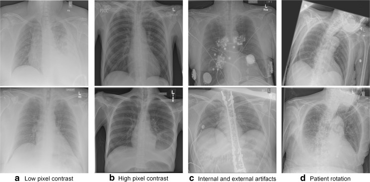
CXRs have a wide variation of appearance in pixel contrast, internal and external artifacts, and patient positioning as presented in Fig. 1. CXRs also have varying resolutions due to the geometry of the source, object, and detector. Our hospital protocol is to perform AP portable radiographs with a source, object, and detector distance of 72 in. Our input CXRs ranged from 1734 × 1782 to 3408 × 4200 pixels with an average size of 2777 × 3213 pixels. This variation prevents predictive models from learning significant and invariant features of PICCs. As a result, a preprocessing module is essential to standardize image quality and dimensions before convolutional neural networks (CNNs) can be trained. The preprocessing module is explained in detail in the “Preprocessing” section.
Fig. 1.
Examples of non-processed chest radiographs to demonstrate the wide variation of image quality. This includes radiographs with a low pixel contrast, b high pixel contrast, c internal and external artifacts, and d patient rotation
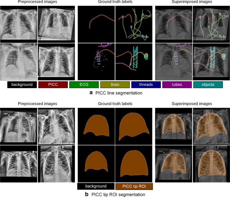
As shown in Fig. 2, label maps for the two different tasks—PICC line and PICC tip ROI segmentation—were created for training and validation datasets (450 cases) by manual annotation by a research assistant with subsequent review by a board-certified radiologist (initials [MHL]). For the purpose of performance evaluation, the correct PICC tip locations were annotated by a radiologist (initials [ST]) on our withheld test dataset (150 cases), as they would be considered ground truth tip locations. The annotation tasks were performed using basic ROI draw functions (brush, polygon, and point) available in OsiriX [13]. The target labels and their corresponding color codes utilized for the segmentation jobs are detailed with descriptions of compositions for each label in Table 1.
Fig. 2.
Input data examples of preprocessed images, ground truth labels, and superimposed images for segmentation of a PICC line and b PICC tip ROI. Seven different semantic labels, including PICC, ECG, lines, threads, tubes, objects, and background, were defined for PICC line segmentation. PICC tip ROI segmentation requires binary labels containing background and PICC tip ROI
Table 1.
Description of labels and color codes used for PICC line and PICC tip ROI segmentation
| Label | Color codes | Description |
|---|---|---|
| PICC line segmentation | ||
| Background PICC |
0 (black) 1 (red) |
Any pixels that any labels are not assigned to PICC lines |
| ECG | 2 (green) | ECG cables |
| Lines | 3 (dark yellow) | Any line-shaped objects excluding PICC and ECG |
| Threads | 4 (blue) | Surgical sutures and staples, used for closing surgical incisions |
| Tubes | 5 (purple) | Any tube-shaped objects |
| Objects | 6 (dark cyan) | Any foreign structures, such as pacemaker devices, simulators, catheter hubs, and ECG electrodes |
| PICC tip ROI segmentation | ||
| Background | 0 (black) | Any pixels that any labels are not assigned to |
| PICC tip ROI | 1 (dark orange) | Subregion of the lung zone excluding the subphrenic areas |
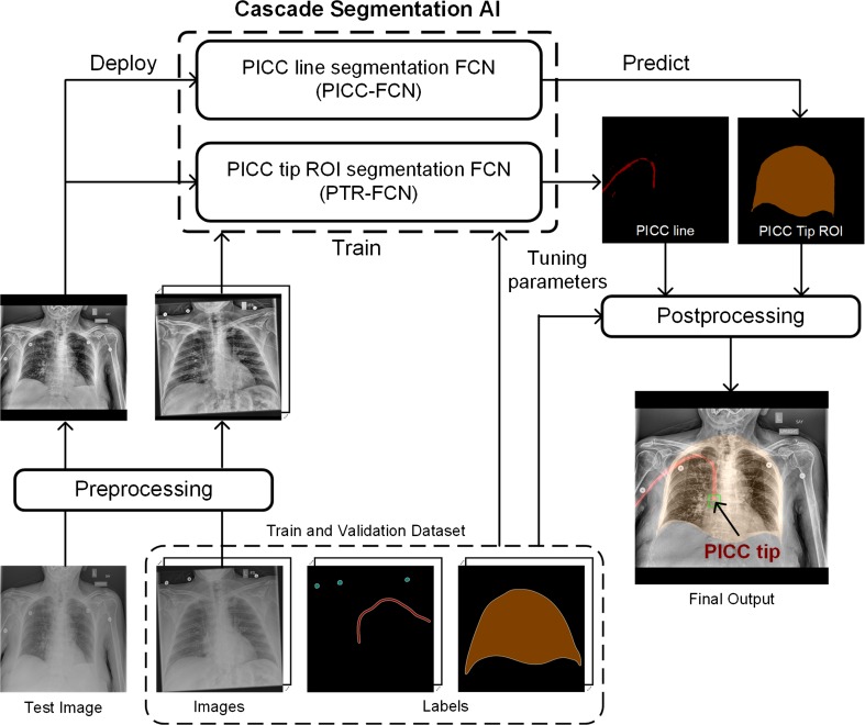
We reformatted the annotated label maps into input labels acceptable for two CNNs for PICC line and PICC tip ROI segmentation, as shown in Fig. 2. The preprocessed images and the corresponding color-coded label maps serve as input images and their pixel-level targets for the two CNNs, respectively. Object boundaries were ignored during training as the pixels surrounding a boundary are ambiguous and can be segmented into any label because of inherent semantic overlap. Figure 3 shows the architecture of the deep-learning system we used in this study.
Fig. 3.
Overview of our proposed fully automated deep-learning system for PICC tip detection. The system consists of a preprocessing module and a cascade segmentation AI containing FCNs for PICC line segmentation FCN (PICC-FCN) and for PICC tip ROI segmentation FCN (PTR-FCN), followed by a post-processing module
System Architecture
Preprocessing
Non-processed AP CXRs are often hazy and have low pixel contrast which prevents CNNs from discriminating PICC from similar appearing objects. Consequently, we took two preprocessing steps to normalize contrast and dimensions of input images. First, Contrast Limited Adaptive Histogram Equalization (CLAHE) [16] was applied to achieve consistency in image contrast. Second, all images were zero-padded to equalize their widths and heights with preserving their aspect ratios, followed by resizing them to 1024 × 1024 pixels. The larger image size was based on our intuition that discriminant features of PICC lines could be lost in image size reduction to more conventional 256 × 256 images. Recent work [17] achieved good segmentation performance of anatomical organs on CXRs despite resizing to 256 × 256 pixels. However, significant features of PICCs could possibly be lost at that size because the widths of PICCs are less than 4 pixels in a 256 × 256 pixel image. As a result, we chose 1024 × 1024 pixels as the size is the largest one our computational hardware could process.
Cascade Segmentation AI: Fully Convolutional Networks
We proposed a cascade architecture of segmentation AI system with two CNNs for segmenting PICC line and its tip ROI as shown in Fig. 3. We chose FCNs among different types of CNNs for three main reasons. FCNs process images and labels in one forward pass for pixel wise segmentations from any-sized input images, allowing us to use 1024 × 1024 pixel images. Using FCNs also allows us to utilize transfer learning by importing a pre-trained model such as ImageNet [18] and accelerate the loss convergence function to a global optimum even when using a small dataset. Moreover, as explained by Long et al. [15], FCN intentionally fuses different levels of layers for the purpose of combining coarse-grained and fine-grained features extracted from earlier and later layers, thus achieving accurate segmentation results thanks to the exploitation of local and global context. Lastly, FCNs can be trained end to end, pixels to pixels with input images and their pixel wise target labels and then be deployed whole-image-at-a-time [15].
Prior work in image classification has used a patch-based approach [19, 20] which requires redundant pixel wise classifications using multiple small patches for each pixel. Our FCN approach outperforms patches because it only performs one forward computation. Unmodified FCNs contain only FCN-32s, FCN-16s, and FCN-8s architectures that fuse and upsample coarse-grained and fine-grained features at granularity of 32, 16, and 8 pixels, respectively [15]. However, we have experimented with finer grained FCN architectures, FCN-4s and FCN-2s, in order to find the optimal granularity of FCN for accurate PICC tip detection.
Post-processing
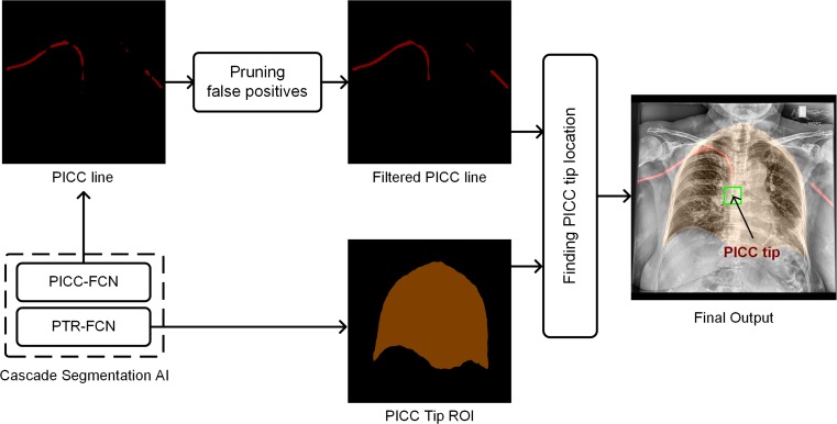
After generating a segmented region of PICC line from PICC-FCN, the system passes it to the post-processing module. Bone edges and other dense linear structures can be erroneously detected as potential false positives. By using a probabilistic Hough line transform algorithm [21], false positives that are distant from the predicted PICC regions are excluded. As shown in Fig. 4, the algorithm effectively merged the significant nearby contours to generate a smoothly curved PICC line trajectory. Our validation dataset facilitated finding optimal combinations of parameters for better algorithmic performance—minimum length of line (minLineLength), maximum allowed gap between line segments for a single line (maxLineGap), and minimum vote count for a line to be formed (minVotingNum). After iterative attempts, using values of minVotingNum = 50, minLineLength = 30, and maxLineGap = 50 provided the best accuracy. After filtering out falsely predicted PICC regions, the catheter tip location can then be computed by simply finding the point with the largest y value inside the PICC tip ROI where the tip is supposed to be located. Final outputs created by our proposed system are shown as a superimposed image with PICC line and its tip location (Fig. 4).
Fig. 4.
Overview of proposed post-processing module for pruning false positives using an optimized Hough line transform algorithm and finding the PICC tip location within the selection ROI predicted by PTR-FCN
Training
We fine-tuned the FCN models after initializing them with pre-trained models retrieved from FCN GitHub [22]. We used a minibatch stochastic gradient descent with momentum 0.9 and a minibatch size of four images. Hyperparameters need to be carefully chosen for a stable convergence to the global optimum when input images are high-resolution (1024 × 1024 pixels). We empirically noticed that using a learning rate of 10−10 and a weight decay of 10−12 enabled a stable convergence of training and validation loss for our application. All experiments were run on a Devbox (NVIDIA Corp, Santa Clara, CA) containing four TITAN X graphics processing units (GPUs) with 12GB of memory per GPU [23], and with Nvidia deep-learning frameworks, including Nvidia-Caffe (0.15.14) and Nvidia DIGITS (5.1).
Model Selection
The best performing FCN models were identified by using Dice similarity coefficient (DSC) results on our validation dataset by increasing granularities of FCN fusions—FCN-32s, FCN-16s, FCN-8s, FCN-4s, and FCN-2s. For PICC tip ROI segmentation FCN (PTR-FCN), FCN-16s model was selected since it achieved the best performance (DSC = 0.968) among the five FCN models. For PICC line segmentation FCN (PICC-FCN), the best FCN models were selected for each FCN model based on its DSC results on the validation dataset. Subsequently, we made comparisons between the entire systems with different FCN models using absolute distance measurements of tip locations on our held-out test dataset.
Results
Performance
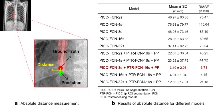
Absolute distance measurement for final performance of our proposed algorithm in this study is visually described in Fig. 5a. Performance comparisons between different models are present with values of mean and standard deviation (mean ± SD) and root mean square error (RMSE) for absolute distances in Fig. 5b. Results are expressed in millimeters based on radiographic pixel spacing using an SID of 72 in. (1 pixel = 0.125 mm). Absolute distances between predicted and ground truth PICC tip locations using only the PICC line segmentation FCN (PICC-FCN) ranged from 28.98 to 78.68 mm (second row in Fig. 5b). Overlaying the PICC tip ROI segmentation FCN (PTR-FCN) system resulted in improved algorithm performance with absolute distances ranging from 3.10 to 23.23 mm (third row in Fig. 5b). Combining the cascade segmentation AIs (PICC-FCN-8s and PTR-FCN-16s) followed by the post-processing module achieved the shortest absolute distances on the test dataset, with a mean of 3.10 mm, a standard deviation of 2.03 mm, and a RMSE of 3.71 mm.
Fig. 5.
Visual description of a absolute distance measurement between predicted and ground truth PICC tip locations and b performance comparisons between PICC line segmentation FCN (PICC-FCN) without and with PICC tip ROI segmentation FCN (PTR-FCN) and post-processing module. Distance values are measured in mm for both of mean ± SD and root mean square error (RMSE)
Deployment Time
Our proposed PICC tip detection system was performed using a single TITAN X GPU for deployment. The best performing system (PICC-FCN-8s + PTR-FCN-16s + PP) took 198 s for testing 150 cases in total. The execution time corresponds to 1.32 s per image, with the following breakdown: 0.22 s of preprocessing, 0.56 s of PICC-FCN, 0.53 s of PTR-FCN, and 0.01 s of post-processing per image.
Image Annotations with Other Labels
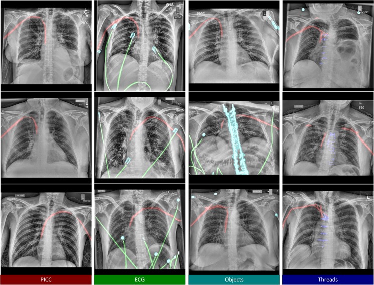
Multiple examples of output images from our PICC-FCN-8s model are detailed in Fig. 6. All images in Fig. 6 highlight the trajectories of the PICCs in red. Images in each column reveal the general cases of annotating multiple external objects, including PICCs, ECGs, electrodes, surgical sutures, and medical devices, each highlighted in different colors (ECG in green, objects in dark cyan, and sutures in blue).
Fig. 6.
Representative result images with annotations of PICC, ECG, internal and external objects, and surgical sutures produced by PTR-PICC in different colors
Mislabeled Cases
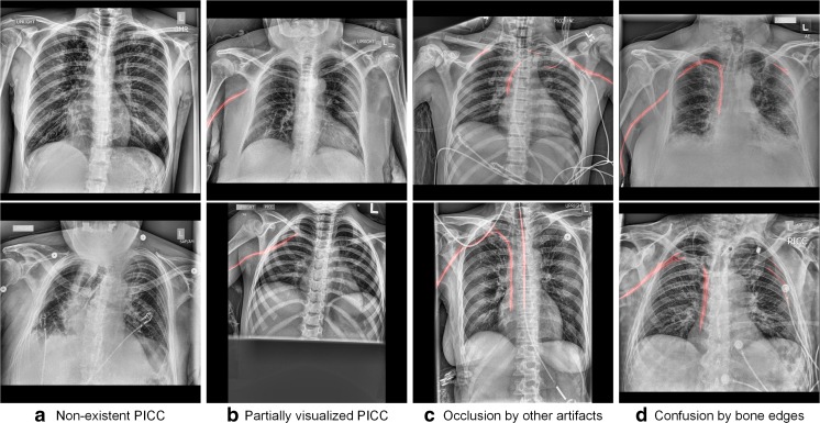
Figure 7 presents example output images for cases where the algorithm was completely incorrect. The images in the first two columns demonstrate that our proposed algorithm can identify cases non-existent or partially visualized PICC cases. The images in the last two columns reveal examples of poor algorithmic performance where false predictions of PICCs occur within the predicted PICC tip ROI. PICCs are challenging to localize when occluded by other similar appearing objects (Fig. 7c) and bone edges (Fig. 7d), causing occasional false positives or negatives.
Fig. 7.
Representative images for exceptional cases. Our proposed system enables identification of a non-existent and b partial PICC visualization. The current algorithm does not perform perfectly when the confusion exists from c other similar appearing artifacts or d edges of bone structures
Discussion
We have developed a fully-automated system for performing PICC line detection and localizing the catheter tip on CXRs using a cascade segmentation AI system with two fully convolutional networks and preprocessing and post-processing modules at a fast deployment time (< 1.3 s per image). We found that using intermediate granularity (FCN-8s and FCN-16s) for segmenting both the PICC trajectory and its tip ROI performed better than using highly granular fully convolutional networks (FCN-2s and FCN-4s). The finer-grained networks probably confuse PICCs with other similar objects when only examining four pixels at a time. Intermediate granularity may have had optimal performance because the width of the typical PICC ranges from 8 to 16 pixels when CXRs were resized to 1024 × 1024 pixels. By combining only hierarchical features at different layers of granularity of 8 to 16 pixels, we may have inadvertently helped the network focus by forcing it to look at objects at a given size range. Much as a forest can be lost for the trees, optimal granularity may prove to be analogous to telling the network how big of a forest to expect.
Data augmentation using random mirroring and image rotation from − 30 to 30° in 5° increments did not provide a noticeable improvement in performance. Our suspicion is that the dataset already representatively contains many similar PICC appearances because PICCs can be inserted on the left or right sides, or the PICC courses along variable trajectories. Non-linear transformations may be able to help neural networks learn more discriminative features from objects with deformed shapes and appearances; however, this investigation is beyond the scope of this work and will be addressed in future directions.
Clinical Applications and Future Directions
Chest radiography performed for PICC tip detection is a frequent exam in the care of sick patients, and it is among the mundane but necessary tasks required in clinical care. Our proposed system can identify a PICC tip’s location in approximately 1.3 s and could help accelerate the recognition of malpositioned catheters.
Our initial intent was to develop a deep-learning system for PICC detection. However, as part of training the models to distinguish PICC from non-PICC, we used many other object labels rather than collapsing all non-PICC objects into a single label. This allows us to further expand the system to identify all lines and tubes frequently used in the clinical setting without having to redesign the system. Future directions will require querying the PACS database for sufficient cases for each of the other classes and annotating those images appropriately so we can independently test the algorithm’s performance for each additional class.
Limitations
While the algorithms have great potential to improve workflow efficiency, there are important limitations. The system often confuses PICCs with bone edges, especially around ribs. This confusion can be reduced by expanding the semantic annotation classes by creating a rib label, passing the new label to the CNNs so they may learn significant features of ribs and their edges, allowing PICCs to be differentiated from bone edges. Performance may also be impaired by linear medical objects. However, ECG cables, external objects, and surgical sutures were well represented in the dataset—120 for ECG, 60 for objects, and 54 for sutures—and therefore are not confused with PICCs (Fig. 6.) We can also train the system to distinguish metal objects from PICC. Another inherent limitation is that most pixels in a CXR derive from the background class [24]. The resulting class imbalance always occurs even despite additional training data. In order to combat the imbalance problem, class frequency weights can be incorporated into the loss function [17] or data augmentation on non-background samples could be performed [25, 26].
Conclusion
We have proposed a deep-learning system to automatically detect the course and tip location of PICCs. The mean predicted location of the PICC tip is 3.10 mm from ground truth with a standard deviation of 2.03 mm and a root mean square error of 3.71 mm. Mean deployment time is only 1.31 s per image when our system is deployed on a single GPU. The system is generalizable to include other types of vascular access and therapeutic support devices, although the system’s efficacy for classification of these objects has not been fully tested in this initial work. It is our hope that this system can help improve patient safety by reducing turnaround time and speeding interpretation of radiographs.
Acknowledgements
The authors gratefully acknowledge Jordan Rogers for his commitment to initial implementation of PICC line detection machine learning system. We thank Junghwan Cho, PhD; Dania Daye, MD; Vishala Mishra, MD; and Garry Choy, MD for their helpful clinical comments.
Contributor Information
Hyunkwang Lee, Email: hlee51@mgh.harvard.edu.
Mohammad Mansouri, Email: mmansouri1@mgh.harvard.edu.
Shahein Tajmir, Email: stajmir@mgh.harvard.edu.
Michael H. Lev, Email: mlev@partners.org
Synho Do, Phone: (617) 643-0247, Email: sdo@mgh.harvard.edu.
References
- 1.Funaki B. Central venous access: a primer for the diagnostic radiologist. AJR Am J Roentgenol. 2002;179:309–318. doi: 10.2214/ajr.179.2.1790309. [DOI] [PubMed] [Google Scholar]
- 2.Fuentealba I, Taylor GA. Diagnostic errors with inserted tubes, lines and catheters in children. Pediatr Radiol. 2012;42:1305–1315. doi: 10.1007/s00247-012-2462-7. [DOI] [PubMed] [Google Scholar]
- 3.Tomaszewski KJ, Ferko N, Hollmann SS, Eng SC, Richard HM, Rowe L, et al. Time and resources of peripherally inserted central catheter insertion procedures: a comparison between blind insertion/chest X-ray and a real time tip navigation and confirmation system. Clinicoecon Outcomes Res. 2017;9:115–125. doi: 10.2147/CEOR.S121230. [DOI] [PMC free article] [PubMed] [Google Scholar]
- 4.Pereira S, Pinto A, Alves V, Silva CA: Brain Tumor Segmentation using Convolutional Neural Networks in MRI Images. IEEE Trans Med Imaging, 2016. 10.1109/TMI.2016.2538465 [DOI] [PubMed]
- 5.Havaei M, Davy A, Warde-Farley D, Biard A, Courville A, Bengio Y, et al. Brain tumor segmentation with Deep Neural Networks. Med Image Anal. 2017;35:18–31. doi: 10.1016/j.media.2016.05.004. [DOI] [PubMed] [Google Scholar]
- 6.Anthimopoulos M, Christodoulidis S, Ebner L, Christe A, Mougiakakou S: Lung Pattern Classification for Interstitial Lung Diseases Using a Deep Convolutional Neural Network. IEEE Trans Med Imaging, 2016. 10.1109/TMI.2016.2535865 [DOI] [PubMed]
- 7.Lee H, Tajmir S, Lee J, Zissen M, Yeshiwas BA, Alkasab TK et al.: J Digit Imaging, 2017. 10.1007/s10278-017-9955-8 [DOI] [PMC free article] [PubMed]
- 8.Greenspan H, van Ginneken B, Summers RM: Guest Editorial Deep Learning in Medical Imaging: Overview and Future Promise of an Exciting New Technique. IEEE Trans Med Imaging 35:1153–1159
- 9.Lakhani P, Sundaram B: Deep Learning at Chest Radiography: Automated Classification of Pulmonary Tuberculosis by Using Convolutional Neural Networks. Radiology 162326, 2017 [DOI] [PubMed]
- 10.Cicero M, Bilbily A, Colak E, Dowdell T, Gray B, Perampaladas K, et al. Training and Validating a Deep Convolutional Neural Network for Computer-Aided Detection and Classification of Abnormalities on Frontal Chest Radiographs. Invest Radiol. 2017;52:281–287. doi: 10.1097/RLI.0000000000000341. [DOI] [PubMed] [Google Scholar]
- 11.Bar Y, Diamant I, Wolf L, Lieberman S, Konen E, Greenspan H: Chest pathology identification using deep feature selection with non-medical training. Computer Methods in Biomechanics and Biomedical Engineering: Imaging & Visualization. Taylor & Francis, 2016, pp 1–5
- 12.Yang W, Chen Y, Liu Y, Zhong L, Qin G, Lu Z, et al. Cascade of multi-scale convolutional neural networks for bone suppression of chest radiographs in gradient domain. Med Image Anal. 2017;35:421–433. doi: 10.1016/j.media.2016.08.004. [DOI] [PubMed] [Google Scholar]
- 13.Chen S, Zhong S, Yao L, Shang Y, Suzuki K. Enhancement of chest radiographs obtained in the intensive care unit through bone suppression and consistent processing. Phys Med Biol. 2016;61:2283–2301. doi: 10.1088/0031-9155/61/6/2283. [DOI] [PubMed] [Google Scholar]
- 14.Lee W-L, Chang K, Hsieh K-S. Unsupervised segmentation of lung fields in chest radiographs using multiresolution fractal feature vector and deformable models. Med Biol Eng Comput. 2016;54:1409–1422. doi: 10.1007/s11517-015-1412-6. [DOI] [PubMed] [Google Scholar]
- 15.Long J, Shelhamer E, Darrell T: Fully convolutional networks for semantic segmentation. In Proceedings of the IEEE Conference on Computer Vision and Pattern Recognition. 2015, pp 3431–3440 [DOI] [PubMed]
- 16.Zuiderveld K.: Contrast Limited Adaptive Histogram Equalization. In Graphics Gems IV. Academic Press Professional, Inc., San Diego, 1994, pp 474–485
- 17.Novikov AA, Lenis D, Major D, Hladůvka J, Wimmer M, Bühler K: Fully Convolutional Architectures for Multi-Class Segmentation in Chest Radiographs [Internet]. arXiv [cs.CV]. Available: http://arxiv.org/abs/1701.08816, 2017 [DOI] [PubMed]
- 18.Deng J, Dong W, Socher R, Li LJ, Li K, Fei-Fei L: ImageNet: A large-scale hierarchical image database. In Computer Vision and Pattern Recognition, 2009. CVPR 2009. IEEE Conference on 2009, pp 248–255
- 19.Platero C, Tobar MC: Combining a Patch-based Approach with a Non-rigid Registration-based Label Fusion Method for the Hippocampal Segmentation in Alzheimer’s Disease. Neuroinformatics, 2017. 10.1007/s12021-017-9323-3 [DOI] [PubMed]
- 20.Ciresan D, Giusti A, Gambardella LM, Schmidhuber J: Deep Neural Networks Segment Neuronal Membranes in Electron Microscopy Images. In: Pereira F, Burges CJC, Bottou L, Weinberger KQ, editors. Advances in Neural Information Processing Systems 25. Curran Associates, Inc. 2012, pp 2843–2851
- 21.Kiryati N, Eldar Y, Bruckstein AM. A probabilistic Hough transform. Pattern Recognit. 1991;24:303–316. doi: 10.1016/0031-3203(91)90073-E. [DOI] [Google Scholar]
- 22.Shelhamer E: fcn.berkeleyvision.org [Internet]. Github; Available: https://github.com/shelhamer/fcn.berkeleyvision.org
- 23.NVIDIA® DIGITS™ DevBox: In: NVIDIA Developer [Internet]. Available: https://developer.nvidia.com/devbox, 16 Mar 2015 [cited 23 Aug 2016]
- 24.Litjens G, Kooi T, Bejnordi BE, Setio AAA, Ciompi F, Ghafoorian M, et al.: A Survey on Deep Learning in Medical Image Analysis [Internet]. arXiv [cs.CV]. Available: https://arxiv.org/abs/1702.05747, 2017 [DOI] [PubMed]
- 25.Kamnitsas K, Ledig C, Newcombe VFJ, Simpson JP, Kane AD, Menon DK, et al. Efficient multi-scale 3D CNN with fully connected CRF for accurate brain lesion segmentation. Med Image Anal. 2017;36:61–78. doi: 10.1016/j.media.2016.10.004. [DOI] [PubMed] [Google Scholar]
- 26.Litjens G, Sánchez CI, Timofeeva N, Hermsen M, Nagtegaal I, Kovacs I, et al. Deep learning as a tool for increased accuracy and efficiency of histopathological diagnosis. Sci Rep. 2016;6:26286. doi: 10.1038/srep26286. [DOI] [PMC free article] [PubMed] [Google Scholar]


