Identifying populations sensitive to environmental chemicals by simulating toxicokinetic variability

Abstract

The thousands of chemicals present in the environment (USGAO 2013) must be triaged to identify priority chemicals for human health risk research. Most chemicals have little of the toxicokinetic (TK) data that are necessary for relating exposures to tissue concentrations that are believed to be toxic. Ongoing efforts have collected limited, in vitro TK data for a few hundred chemicals. These data have been combined with biomonitoring data to estimate an approximate margin between potential hazard and exposure. The most “at risk” 95^th percentile of adults have been identified from simulated populations that are generated either using standard “average” adult human parameters or very specific cohorts such as Northern Europeans. To better reflect the modern U.S. population, we developed a population simulation using physiologies based on distributions of demographic and anthropometric quantities from the most recent U.S. Centers for Disease Control and Prevention National Health and Nutrition Examination Survey (NHANES) data. This allowed incorporation of inter-individual variability, including variability across relevant demographic subgroups. Variability was analyzed with a Monte Carlo approach that accounted for the correlation structure in physiological parameters. To identify portions of the U.S. population that are more at risk for specific chemicals, physiologic variability was incorporated within an open-source high-throughput (HT) TK modeling framework. We prioritized 50 chemicals based on estimates of both potential hazard and exposure. Potential hazard was estimated from in vitro HT screening assays (i.e., the Tox21 and ToxCast programs). Bioactive in vitro concentrations were extrapolated to doses that produce equivalent concentrations in body tissues using a reverse dosimetry approach in which generic TK models are parameterized with: 1) chemical-specific parameters derived from in vitro measurements and predicted from chemical structure; and 2) with physiological parameters for a virtual population. For risk-based prioritization of chemicals, predicted bioactive equivalent doses were compared to demographic-specific inferences of exposure rates that were based on NHANES urinary analyte biomonitoring data. The inclusion of NHANES-derived inter-individual variability decreased predicted bioactive equivalent doses by 12% on average for the total population when compared to previous methods. However, for some combinations of chemical and demographic groups the margin was reduced by as much as three quarters. This TK modeling framework allows targeted risk prioritization of chemicals for demographic groups of interest, including potentially sensitive life stages and subpopulations.

1. Introduction¹

The U.S. Environmental Protection Agency (EPA) is responsible for determining risks associated with chemicals in the environment. In order to address the thousands of man-made chemicals present in environmental samples (Rager et al. 2016) and human blood (Park et al. 2012), the EPA requires efficient risk-based methods to prioritize, screen, and evaluate chemicals. A promising framework for prioritization (Thomas et al. 2013; Wetmore et al. 2015) identifies chemicals with greater putative risk by combining data from high-throughput in vitro toxicity screening (HTS) assays, such as those developed and used by the US EPA ToxCast program (Kavlock et al. 2012), with data from high-throughput exposure modeling frameworks, such as US EPA ExpoCast (Wambaugh et al. 2013; Wambaugh et al. 2014). Those chemicals more likely to pose a risk become targets for further investigation.

In vitro bioactivity HTS has been conducted for thousands of chemicals to date (Kavlock et al. 2012). To use in vitro HTS for chemical prioritization, methods for in vivo-in vitro extrapolation (IVIVE) have been developed that relate external chemical exposures to internal tissue concentrations (Aylward and Hays 2011; Rotroff et al. 2010). A primary application of IVIVE in risk prioritization has been reverse dosimetry, which uses toxicokinetic (TK) modeling to predict the oral equivalent dose (OED) of a chemical needed to produce an internal (e.g., plasma) concentration equal to a bioactive in vitro concentration (Rotroff et al. 2010; Tan et al. 2007; Tan et al. 2006). The ratio of OED to estimated human exposure is a measure of potential risk (Judson et al. 2011; Thomas et al. 2013); this ratio is known as the activity-exposure ratio, or AER.

Unfortunately, unlike the thousands of chemicals with predicted estimates for toxicity and exposure, TK data from traditional methods are available for only a few dozen chemicals (Wetmore et al. 2015; Wetmore et al. 2012). Alternative in vitro methods for TK have allowed the development of very simple prototype TK models for many hundreds of chemicals (Rotroff et al. 2010; Wetmore et al. 2015; Wetmore et al. 2012). These simple “high throughput” TK (HTTK) models are useful precisely because they are simple – they can be rapidly parameterized using in vitro measurements of chemical clearance by hepatocytes and plasma protein binding (Rotroff et al. 2010) as well as bioavailability data (Wetmore et al. 2012). With additional data, more elaborate models have been generated (Wambaugh et al. 2015), including simulation of population variability in metabolizing enzymes (Wetmore et al. 2014). However, these data cannot currently be rapidly generated for large numbers of chemicals. The minimal HTTK data used for characterizing chemicals constrains models built on these data in how they may describe variability between individuals. However, these HTTK data and models have been useful for identifying those chemicals that are more likely to pose a human health risk (Thomas et al. 2013; Tonnelier et al. 2012; USEPA 2014; Wetmore et al. 2015; Wetmore et al. 2012).

TK, hazard, and exposure are known to vary between individuals, life stages, and populations with varying genetics, ontogeny, and physiology (Belle and Singh 2008; Hines 2007; Jamei et al. 2009a; Lipscomb and Kedderis 2002; McNally et al. 2014; Wambaugh et al. 2014). Therefore, to better describe vulnerable life stages and populations, HT risk-based chemical prioritization needs to incorporate inter-individual variability in predictions of both hazard and exposure. The open-source, publicly available R package ‘httk’ (hereafter referred to as “HTTK-package”), was developed to facilitate HTTK modeling for IVIVE (Pearce et al. 2016). Currently, the HTTK-package incorporates the ability to simulate inter-individual physiological variability by Monte Carlo (MC) sampling of the HTTK model parameters using uncorrelated normal distributions characterized by means and coefficients of variation (Wambaugh et al. 2015); these distributions typically reflect the physiology of a healthy young Caucasian adult (Birnbaum et al. 1994; Valentin 2002).

Here, we incorporate the inter-individual variability of the modern U.S. population into high-throughput risk-based chemical prioritization. To do this, we develop a population physiology simulation that makes demographic-specific predictions of chemical risk, using data collected as part of the ongoing National Health and Nutrition Examination Survey (NHANES) performed by the Centers for Disease Control (CDC) (http://www.cdc.gov/nchs/nhanes.htm) (Johnson et al. 2014). This new tool, which we refer to here as “HTTK-Pop,” has been publicly released for use by the TK and risk assessment communities.

HTTK-Pop uses a correlated MC approach to simulate inter-individual physiological variability across demographic groups. We evaluate our approach using predictions of steady-state plasma concentrations (C_ss) derived from in vivo measurements for 95 pharmaceutical (Obach et al. 2008) and other (Wetmore et al. 2012) compounds. We further assess predictions of inter-individual variability in C_ss using published in vivo measurements from 86 studies of 14 compounds (Howgate et al. 2006; Johnson et al. 2006).

We demonstrate the impact of human variability using an example framework for chemical risk prioritization (Wetmore et al. 2015). We simulate ten important demographic groups of the U.S. population informed by the NHANES. For each demographic group, we use chemical bioactivity HTS data and our new description of physiology for individuals within each demographic to predict the population distributions of doses needed to cause bioactivity for 50 chemicals. We then estimate the group-specific AERs as a measure of potential risk. Finally, we identify chemicals and groups within the U.S. population with greater predicted risk of chemical exposure-induced bioactivity, as characterized by high throughput methods.

2. Methods

2.1. High Throughput Toxicokinetics data

All the TK data and models for HTTK-Pop used in this analysis are open source and publicly available as R package “httk” (Pearce et al. 2016) v1.5. This version included literature data on 543 chemicals, but our analysis was limited to 50 chemicals for which both HTS bioactivity data (Section 2.8) and exposure inferences (Section 2.9) were available. In the HTTK-package the chemicals are described by physico-chemical properties (molecular weight and hydrophobicity) obtained from EPI Suite (USEPA), as well as ionization equilibria (Strope et al. 2015). The chemicals are further described by in vitro measurements of pooled human hepatocyte clearance and plasma protein binding, as in Wetmore et al. (2015; 2012). Absorption is assumed to be fast (1/h) and bioavailability is assumed to be 100%. The MC population simulation methods included in previous versions of the HTTK-package were replaced in version 1.5 by the HTTK-Pop methods described here.

2.2. Model used for reverse TK

The HTTK-package includes several TK models. For our analysis, we used a general TK model from previous HT risk prioritization studies (Wetmore et al. 2014; Wetmore et al. 2015; Wetmore et al. 2012) to predict steady-state plasma concentrations (C_ss):

$$C_{ss}= \frac{k_o}{\left(GFR \times F_{ub}\right)+\frac{Q_{liver}\times F_{ub}\times C{L}_{int, h}}{Q_{liver}+F_{ub}\times C{L}_{int, h}}}$$ Equation 1

In Equation 1, k_o represents the dose rate (mg/kg/h); F_ub, the fraction of parent compound unbound in blood; Q_liver, the hepatic portal vein blood flow per kg body weight (L/h/kg); GFR, the glomerular filtration rate per kg body weight (L/h/kg); CL_int,h, the whole-liver intrinsic clearance rate per kg body weight under first-order metabolism conditions (L/h/kg). The model is equivalent to the steady-state concentration in a three-compartment (liver, gut, and body blood) model. It assumes zero-order uptake of a daily dose from the gut with 100% oral bioavailability, includes passive renal clearance, and assumes a first-order hepatic clearance modeled using the “well-stirred” approximation (Wilkinson and Shand 1975). Because this model is a steady-state model (i.e., sufficient time has passed for free chemical concentration in plasma to equilibrate with all tissues) tissue partitioning is not included in Equation 1. This model has been shown to predict C_ss similarly to a more detailed, perfusion-limited PBTK model for all but a few highly bioaccumulative compounds (Wambaugh et al. 2015). The model includes both physiological parameters (GFR and Q_liver) and chemical-specific parameters (F_ub and CL_int.h). When chemical-specific estimates of F_ub and CL_int,h are available, the model can be parameterized for that chemical.

F_ub was estimated from in vitro measurements of the fraction of chemical unbound in plasma (F_up), by assuming a constant ratio of blood concentration to plasma concentration (R_b2p).

$$F_{ub}=\frac{F_{up}}{R_{b2p}}$$ Equation 2

R_b2p was in turn calculated according to Equation 3, using hematocrit (Hct) and the partition coefficient between red blood cells and plasma (K_RBC2p). K_RBC2p was predicted from physico-chemical properties using Schmitt’s method (Schmitt 2008).

$$R_{b2p}=\text{1 - Hct }+ \text{Hct}\times K_{RBC2p}\times F_{up}$$ Equation 3

Whole-organ intrinsic hepatic clearance per kg body weight (CL_int,h) was scaled from intrinsic clearance rates measured in vitro in human hepatocytes (CL_int) using the following equation:

$$C{L}_{int,h}=C{L}_{int}\times \text{hepatocellularity ×}{M}_{liver}$$ Equation 4

where M_liver represents liver mass in kg, and hepatocellularity is millions of cells per kg of liver tissue.

2.3. Simulating inter-individual variability in the TK model

To simulate inter-individual variability in the TK model, a MC approach is used: the model parameters are sampled from known or assumed distributions, and the model is evaluated for each sampled set of parameters. To simulate variability across subpopulations, the MC approach needs to capture the parameter correlation structure. For example, kidney function changes with age (Levey et al. 2009), thus the distribution of GFR is likely different in 6-year-olds than in 65-year-olds.

To directly measure the parameter correlation structure, all parameters need to be measured in each individual in a representative sample population. Such direct measurements are extremely limited. However, the correlation structure of the physiological parameters can be inferred from their known individual correlations with demographic and anthropometric quantities for which direct population measurements do exist. These quantities are sex, race/ethnicity, age, height, and weight (Howgate et al. 2006; Jamei et al. 2009a; Johnson et al. 2006; McNally et al. 2014; Price et al. 2003). Direct measurements of these quantities in a large, representative sample of the U.S. population are publicly available from NHANES. NHANES also includes laboratory measurements, including both serum creatinine, which can be used to estimate GFR (Levey et al. 2009), and hematocrit. For conciseness, sex, race/ethnicity, age, height, weight, serum creatinine, and hematocrit will be called the NHANES quantities.

HTTK-Pop’s correlated MC approach begins by sampling from the joint distribution of the NHANES quantities to simulate a population. Then, for each individual in the simulated population, HTTK-Pop predicts the physiological parameters in Equations 1–4 from the NHANES quantities using regression equations from the literature (Barter et al. 2007; Baxter‐Jones et al. 2011; Bosgra et al. 2012; Koo et al. 2000; Levey et al. 2009; Looker et al. 2013; McNally et al. 2014; Ogiu et al. 1997; Price et al. 2003; Schwartz and Work 2009; Webber and Barr 2012). Correlations among the physiological parameters are induced by their mutual dependence on the correlated NHANES quantities. Finally, residual variability is added to the predicted physiological parameters using estimates of residual marginal variance (i.e., variance not explained by the regressions on the NHANES quantities) (McNally et al. 2014).

2.4. Pre-processing NHANES data for use in HTTK-Pop

Data were combined from the three most recent publicly-available NHANES cycles: 2007–2008, 2009–2010, and 2011–2012. For each cycle, some NHANES quantities — height, weight, serum creatinine, and hematocrit — were measured only in a subset of respondents. Only these subsets were included in HTTK-Pop. The pooled subsets from the three cycles contained 29,353 unique respondents. Some respondents were excluded from analysis: those with age recorded as 80 years (because all NHANES respondents 80 years and older were marked as “80”); those with missing height, weight or hematocrit data; and those aged 12 years or older with missing serum creatinine data. These criteria excluded 4807 respondents, leaving 24,546 unique respondents; their breakdown by race/ethnicity and sex is given in Table 1. Each NHANES respondent was assigned a cycle-specific sample weight, which can be interpreted as the number of individuals in the total U.S. population represented by each NHANES respondent in each cycle (Johnson et al. 2013). Because data from three cycles were combined, the sample weights were rescaled (divided by the number of cycles being combined, as recommended in NHANES data analysis documentation) (Johnson et al. 2013). To handle the complex NHANES sampling structure, the R survey package was used to analyze the NHANES data (Lumley 2004). More details of NHANES data processing are available in the Supplementary Material (Section S1.1).

Table 1.

Number of NHANES respondents included in HTTK-Pop dataset, by race/ethnicity and sex.

	Male	Female	Total
Mexican American	2514	2484	4998
Other Hispanic	1358	1450	2808
Non-Hispanic White	4666	4466	9132
Non-Hispanic Black	2705	2744	5449
Other	1092	1067	2159
Total	12335	12211	24546

To allow generation of virtual populations specified by weight class, we coded a categorical variable for each NHANES respondent. The categories Underweight, Normal, Overweight, or Obese were assigned based on weight, age, and height/length (Grummer-Strawn et al. 2010; Kuczmarski et al. 2002; Ogden et al. 2014; WHO 2006; 2010). More details about weight class are available in the Supplementary Material (Section S1.1.7).

2.5. HTTK-Pop algorithms for sampling NHANES quantities

We implemented two population simulation methods within HTTK-Pop: the direct-resampling method and the virtual-individuals method. The direct-resampling method simulated a population by sampling NHANES respondents with replacement, with probabilities proportional to the sample weights. Each individual in the resulting simulated population was an NHANES respondent, identified by a unique NHANES sequence number. By contrast, the second method generates “virtual individuals” — sets of NHANES quantities that obey the approximate joint distribution of the NHANES quantities (calculated using weighted smoothing functions and kernel density estimators; see Section S1.2.2 in the Supplementary Material), but do not necessarily correspond to any particular NHANES respondent. The direct-resampling method removed the possibility of generating unrealistic combinations of the NHANES quantities; the virtual-individuals method allowed the use of interpolation to simulate subpopulations represented by only a small number of NHANES respondents. Further details are given in the Supplementary Material (Section S1.2). For either method, HTTK-Pop takes optional specifications about the population to be simulated (Table 2) and then samples from the appropriate conditional joint distribution of the NHANES quantities.

Table 2.

HTTK-Pop specifications on population to be simulated.

Input	Description	Default if not specified
N	Number of individuals in population.	—
Gender specification	Number of males and females in population.	Both genders included in their proportions in NHANES data, conditional on any other specifications.
Race/ethnicity	One or more of the NHANES race/ethnicity category names (see Table 1)	All race/ethnicity categories included in their proportions in NHANES data, conditional on any other specifications.
Age limits (years)	Minimum and maximum age in years.	If age limits in months specified, then equivalent limits in years; otherwise ages 0–79 years included in their proportions in NHANES data, conditional on any other specifications.
Age limits (months)	Minimum and maximum age in months.	If age limits in years specified, then equivalent limits in months; otherwise ages 0–959 months included in their proportions in NHANES data, conditional on any other specifications.
Weight class	One or more of the weight class category names Underweight, Normal, Overweight, or Obese.	All weight classes included in their proportions in NHANES data, conditional on any other specifications.

Once HTTK-Pop has simulated a population characterized by the NHANES quantities, the physiological parameters of the TK model (Equation 1–4) are predicted from the NHANES quantities using regression equations from the literature. Liver mass was predicted for individuals over age 18 using allometric scaling with height from Reference Man (ICRP 2002), and for individuals under 18 using regression relationships with height and weight published by Ogiu et al. (1997). Residual marginal variability was added for each individual as in PopGen (McNally et al. 2014). Similarly, hepatic portal vein blood flows (in L/h) are predicted as fixed fractions of a cardiac output allometrically scaled with height from Reference Man (ICRP 2002), and residual marginal variability is added for each individual (McNally et al. 2014). Glomerular filtration rate (GFR) (in L/h/1.73 m² body surface area) is predicted from age, race, sex, and serum creatinine using the CKD-EPI equation, for individuals over age 18 (Levey et al. 2009). For individuals under age 18, GFR is estimated from body surface area (BSA) (Johnson et al. 2006); BSA is predicted using Mosteller’s formula (Verbraecken et al. 2006) for adults and Haycock’s formula (Haycock et al. 1978) for children. Hepatocellularity (in millions of cells per gram of liver tissue) is predicted from age using an equation developed by Barter et al. (2007). Hematocrit is estimated from NHANES data for individuals 1 year and older. For individuals younger than 1 year, for whom NHANES did not measure hematocrit directly, hematocrit was predicted from age in months, using published reference ranges (Lubin 1987).

2.6. Inter-individual variability in chemical-specific parameters

In addition to the HTTK physiological parameters, the HTTK models include chemical-specific parameters representing the fraction of chemical unbound in blood (F_ub) and intrinsic clearance (CL_int). Because these parameters represent interactions of the chemical with the body, their values will vary between individuals. To simulate this variability, F_ub and CL_int were included in MC simulations, by sampling from estimated or assumed distributions for the parameters defining them (Equations 2, 3, and 4).

Variability in hematocrit was simulated either using NHANES data (for individuals ages 1 and older) or using age-based reference ranges (for individuals under age 1). F_up was treated as a random variable obeying a distribution censored below the average limit of quantification (LOQ) of the in vitro assay. Specifically, F_up was assumed to obey a normal distribution truncated below at 0 and above at 1, centered at the F_up value measured in vitro, with a 30% coefficient of variation. Below the average LOQ (0.01), F_up was instead drawn from a uniform distribution between 0 and 0.01. F_up was assumed to be independent of all other parameters. This censored normal distribution was chosen to match that used in Wambaugh et al. (2015).

Variability in hepatocellularity (10⁶ cells/g liver) and M_liver (kg) were simulated. The remaining source of variability in CL_int,h is variability in CL_int, which was simulated using a Gaussian mixture distribution to represent the population proportions of poor metabolizers (PMs) and non-PMs of each substance. The true prev alenceof PMs is isozyme-specific (Ma et al. 2002; Yasuda et al. 2008); however, isozyme-specific metabolism data were not available for the majority of chemicals considered. We therefore made a simplifying assumption that 5% of the population are PMs, metabolizing each substance ten times slower than average.

With 95% probability, CL_int was drawn from a non-PM distribution: a normal distribution truncated below at zero, centered at the value measured in vitro, with a 30% coefficient of variation. With 5% probability, CL_int was drawn from a PM distribution: a truncated normal distribution centered on one-tenth of the in vitro value with 30% CV. Both CL_int itself and the probability of being a PM were assumed to be independent of all other parameters. The truncated normal non-PM distribution was chosen because it has been used (with 100% probability) in previous work (Rotroff et al. 2010; Wambaugh et al. 2015; Wetmore et al. 2014; Wetmore et al. 2015; Wetmore et al. 2012); the PM distribution was chosen to comport with the non-PM distribution.

2.7. Methodology for TK Variability Model Evaluation

To evaluate the model’s ability to predict the population median clearance, we compared median model-predicted C_ss values to C_ss values derived from published median in vivo clearance values (Obach et al. 2008) for 95 chemicals. The HTTK-Pop median C_SS was predicted using Equation 1 for each chemical. Because Obach et al. (2008) selected for studies performed in healthy adult populations, model predictions were made for a non-obese population aged 20–50 years (N=1000). HTTK-Pop was used in direct-resampling mode to simulate this population. C_ss values were derived from published median in vivo clearance values by assuming steady state and 100% oral bioavailability; for a dose rate of 1 mg/kg/day, Css was then calculated according to Equation 5.

$$C_{ss}=\frac{\text{dose, }1 \text{mg/kg/day}}{\text{clearance, L/day/kg}}$$ Equation 5

C_ss was converted from units of mg/L to μM using the molecular weight of the compound in question.

To evaluate the model’s ability to predict population variability in clearance, we compared model-predicted variability in clearance to in vivo measurements of inter-individual variability in clearance compiled by Howgate et al. (2006) and Johnson et al. (2006). Howgate et al. compiled data on clearance median and 90% CI (in units of L/h) from in vivo human studies of 15 pharmaceuticals, dosed by both IV and oral routes. Johnson et al. compiled data on clearance median and 95% CI (in units of L/h/kg bodyweight) from in vivo human studies of 11 pharmaceuticals, dosed by both IV and oral routes. (For consistency, we converted the 90% CIs reported in Howgate et al. to 95% CIs, assuming log-normal distributions.) The compiled data tables in Howgate et al. and Johnson et al. characterize each in vivo study by the total number of subjects, their age range, and for some studies, the number of female subjects. For some combinations of chemical and dosing route, clearance data from multiple studies were pooled. In these cases, the compiled data table reported the overall median and CI of clearance, and the number, age range, and/or gender proportion of the combined study populations (Howgate et al. 2006; Johnson et al. 2006). In total, Howgate et al. reported 25 values for 15 chemicals, and Johnson et al. reported 61 values for 11 chemicals.

For each study or pool of studies, in vivo clearance medians and CI bounds were converted into corresponding C_ss values using Equation 5. Clearance measurements in L/h/kg (from Johnson et al.) were converted into C_ss in μM; clearance measurements in L/h (from Howgate et al.) were converted into C_ss in μM/kg. (Because the studies reported in Howgate et al. and Johnson et al. did not report the body weights of their subjects, the units of their reported clearance median and CIs could not be harmonized.)

Model predictions of C_ss variability were made for each reported study or pool of studies. Model simulations were performed using the protocol of Howgate et al. (2006): 20 different “trials” of the study population were simulated for each study, using the virtual-individuals method. For each simulated individual, HTTK-Pop predicts C_ss in units of μM (equivalent to mg/L). Consequently, for comparison to in vivo-derived values from Howgate et al. in units of μM/kg, HTTK-Pop C_ss predictions were divided by the body weight of each simulated individual. For comparison to in vivo-derived values from Johnson et al. in units of μM, HTTK-Pop C_ss predictions were left in their original units. For each study, the overall C_ss median was computed as the median of the 20 trial medians. The predicted C_ss median and 95% CI were then compared to in vivo-derived values. One study of midazolam in neonates (gestational age 28 weeks) (compiled in Johnson et al.) was excluded from the comparison, due to insufficient data for simulation of the neonatal life stage.

To determine the sensitivity of C_ss to the parameters of Equations 1–4, including the physiological parameters (bodyweight, GFR, hepatic portal vein blood flow, hematocrit, hepatocellularity, and liver mass), F_ub, and CL_int, a global sensitivity analysis was performed using the method of Glen and Isaacs (Glen and Isaacs 2012) for each chemical in the data set. This method for variance-based sensitivity analysis computes the Sobol indices as correlation coefficients between pairs of independent MC runs; furthermore, it introduces correction terms to reduce numerical error in the computed Sobol indices arising from spurious correlations (Glen and Isaacs 2012). In this analysis, the first-order sensitivity index for parameter i, S_i, gives the fraction of variability in C_ss that is attributable to variability in that parameter alone (disregarding its interactions with other parameters). S_i can also be interpreted as the expected fractional reduction of variance in C_ss that would be obtained if parameter i could be fixed (Saltelli et al. 2010).

The analysis calculated first-order C_ss sensitivity to CL_int, to F_ub, and to the physiological parameters as a group. Sensitivity could only be determined to the physiological parameters as a group, because the HTTK-Pop-simulated physiological parameters are not independent of one another, but as a group they are independent of F_ub and CL_int (Jacques et al. 2006). (To explore potential sensitivity to individual physiological parameters, another global sensitivity analysis was performed using the assumption that the physiological parameters were independently distributed about “average” values representing an adult Caucasian male. However, the results of this sensitivity analysis are not guaranteed to be representative of the sensitivity of HTTK-Pop-predicted C_ss.)

2.8. ToxCast Bioactivity Data

OEDs were estimated for the bioactive ToxCast concentrations using data from the Aggregated Computational Toxicology Repository (http://www.epa.gov/actor/), downloaded on June 2, 2015). The data are described in Kavlock et al. (2012). In HTS, each chemical is tested in concentration-response across many in vitro assay endpoints. ToxCast data included activity calls (active/inactive) and, if active, the concentration that caused 50% of any observed activity (AC₅₀ values) for 821 different bioactivity assays across 1860 chemicals. The distribution of AC₅₀ across active assays for each chemical approximates the distribution of internal concentrations of that chemical at which various biological effects may occur. This distribution was characterized by 10^th and other percentiles of the ToxCast AC₅₀ values. OEDs were computed using the 95^th percentile C_ss value (denoted C_ss⁹⁵), using reverse dosimetry assuming first-order metabolism (Rotroff et al. 2010).

$$\text{OED}=\frac{{\text{ToxCast AC}}_{50} \text{percentile}}{C_{ss}^{95}}\times 1\text{mg}/\text{kg}/\text{day}$$ Equation 6

These OEDs reflect the dose that would be needed in the most-sensitive 5% of the population to produce a steady-state plasma concentration equal to a given percentile of the ToxCast AC₅₀ distribution across assays for the given chemical. The 10^th percentile AC₅₀ is intended to be a stable (i.e., unlikely to be an outlier) and conservative (i.e., sensitive or potent) estimate of in vitro bioactive concentration: the very lowest AC₅₀ values across assays may reflect noise or otherwise spurious data, and the 10^th percentile is judged likely to exclude these spurious values.

2.9. Exposure Inferences for Demographic subgroups

We performed prioritization for 50 chemicals (Table 4) across ten demographic groups with exposures rates (mg/kg BW/day) that were determined in a previously published high-throughput exposure analysis (Wambaugh et al. 2014). Briefly, a manually-curated metabolic mapping of NHANES urine chemical analytes to chemicals was used to draw inferences of human exposure for each NHANES subject. Bayesian statistical analysis estimated a log-normal parent chemical exposure distribution consistent with the analyte concentrations measured by NHANES. The distribution for each chemical was described by a geometric mean. Analyte measurement limits of detection and uncertainty in the case of analytes and parent chemicals with multiple linkages (i.e., two metabolites shared by three parent chemicals) were considered (Wambaugh et al. 2014).

Table 4.

Enumeration of chemical-specific data for risk prioritization

Data Set	Type of Data	Source	Number of Chemicals
ToxCast	In vitro bioactivity assays	ACToR (Kavlock et al. 2012)	1860
HTTK	In vitro toxicokinetics and physico-chemical properties	HTTK-package v1.5	543
ExpoCast	Exposure rates inferred from NHANES urine metabolites	SupplementalTable-NHANESInferences.xlsx (Wambaugh et al. 2014)	106
Overlapping Chemicals			50

The chemicals used here are only those chemicals for which the median was above the limit of detection. The inferred exposure rates analyzed here are distinct from the heuristic model exposure predictions reported for 7968 chemicals in Wambaugh et al. (2014) – these are the exposures inferred directly from the NHANES data that served as a “training set” for the heuristic model. These data are provided in the supplemental file SupplementalTable-NHANESInferences.xlsx.

2.10. Calculating Activity:Exposure Ratio (AER) for Specific Demographic Groups

As described in Table 4, we restricted our analysis to the 50 chemicals with HTS, exposure, and HTTK data (Sections 2.1 and 2.9, above). Exposures had been inferred for 106 parent chemicals from NHANES urine biomonitoring data (Wambaugh et al. 2013). A total of 51 of these chemicals also had in vitro measurements of hepatocyte clearance and plasma protein binding allowing parameterization of the HTTK models; 50 of those 51 chemicals were included in the most recent ToxCast public release as of this writing (downloaded on June 2, 2015).

HTTK-Pop was used in direct-resampling mode to generate ten simulated populations corresponding to the ten demographic groups, each containing N = 1000 individuals. For each of the ten demographic groups, population variability in steady-state plasma concentration (C_ss) was predicted for each individual and chemical. To characterize the population distribution of C_ss for each chemical, median and 95^th percentiles were computed. For each of those 50 chemicals, the OED was compared to the inferred median exposure rate by computing the activity-exposure ratio, or AER, as defined in (Wetmore et al. 2012).

$$\text{AER}=\frac{\text{OED}}{\text{Inferred exposure}}$$ Equation 7

An AER less than or equal to 1 implies that the estimated exposure is greater than or equal to the dose needed to induce bioactivity. An AER greater than 1 implies that the estimated exposure is lower than the dose needed to induce bioactivity.

3. Results

3.1. Evaluation of Population Simulation Method

There are five key physiological parameters in our TK model: hepatocellularity, GFR, portal vein flow, liver mass, and hematocrit. The CDC NHANES measures four biometrics which may be predictive of these parameters: age, weight, height, and serum creatinine. Based upon the NHANES biometrics, various models (see Methods) allow prediction of the population distribution of our key TK model parameters (Barter et al. 2007; Baxter‐Jones et al. 2011; Bosgra et al. 2012; Koo et al. 2000; Levey et al. 2009; Looker et al. 2013; Ogiu et al. 1997; Price et al. 2003; Schwartz and Work 2009; Webber and Barr 2012).

Figure 1 visualizes the distribution of and relationship between the key model parameters and NHANES biometrics. Figure 1 is a plot matrix of estimated one- and two-dimensional marginal densities of the parameters. These plots illustrate the estimated correlation structure for N=1000 individuals in the NHANES age 20–65 demographic group. The off-diagonal plots (i.e., two-dimensional marginal densities) indicate a noticeable correlation whenever a systematic trend (i.e., a line with non-zero slope) is observed, as opposed to a circular cloud indicating no relationship. A formal calculation of correlation with Bonferroni correction for multiple comparisons indicates that 24 of the 36 pair-wise combinations are significantly correlated (p < 0.05), though only 4 have correlation greater than 0.5. The most notable correlation is height with all parameters except age and GFR. GFR and hepatocellularity were themselves correlated, induced by the fact that both GFR and hepatocellularity generally decrease with age in adults. Body weight also has a slight positive correlation with portal vein flow and liver mass, induced by the fact that these three quantities all generally increase with height in adults.

Figure 1.

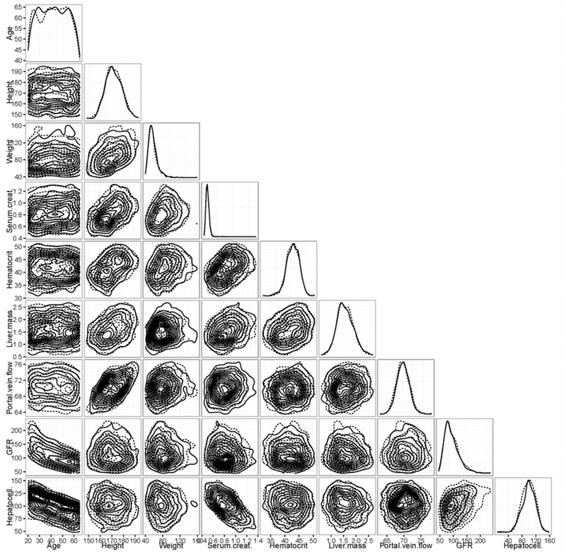
Plot matrix of pairwise density estimates of the parameters generated by HTTK-Pop, for a simulated population Ages 20–65 (N=1000). Solid lines represent data generated using the direct-resampling method; dotted lines represent data generated using the virtual-individuals method. Plot diagonal shows estimated one-dimensional marginal densities. Lower triangular portion of plot shows estimated contours of two-dimensional marginal densities for each pair of parameters. Deviations from concentric circles indicate correlation and/or departure from normal distribution.

The diagonal entries in Figure 1 show the distribution of values across the simulated population (i.e., one-dimensional density). Populations were generated by both the direct-resampling method (actual NHANES subjects, plotted with solid lines) and the virtual-individuals method (plotted with dashed lines) are shown. Direct sampling might be preferred when NHANES includes a large number of actual subjects reflecting the demographic under study (e.g., non-obese adults aged 20–50 years), and was used to evaluate HTTK-Pop model’s ability to predict the population median C_ss. The virtual-individuals method might be preferred for simulation of a more narrowly specified demographic, and was used to evaluate HTTK-Pop’s ability to predict variability in C_ss measured in specific in vivo study populations. As indicated by Figure 1, we did not observe significant differences in the populations generated by these two methods.

In Figure 2, the HTTK-Pop model’s ability to predict the population median C_ss is evaluated by comparison of predicted values to values derived from peer-reviewed literature. The HTTK-Pop median C_SS was predicted using Equation 1 for 95 chemicals, shown on the Y-axis of Figure 2. Each of the 95 chemicals in Figure 2 had in vivo derived C_ss values reported in Wambaugh et al. (2015), shown on the X-axis.

Figure 2.

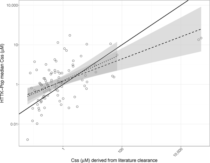
Median C_ss predicted using a generated population of N=1000 non-obese 20–50-year-olds, plotted against median C_ss derived from clearance values measured in vivo for 95 chemicals. Solid line: identity line. Dashed line: best-fit line to the full data set (log₁₀-transformed) (adjusted R²=0.3; intercept 0.16±0.08; slope 0.56±0.09). Dotted line: best-fit line to the log₁₀-transformed data set excluding the two chemicals with the highest literature-derived median C_ss (PFOS and PFOA) (adjusted R² = 0.22; intercept 0.2±0.09; slope 0.67±0.13). Shaded regions around each line denote the 99% confidence intervals around each fit.

A regression of the measured data on the predictions in Figure 2 indicates that HTTK-Pop has limited ability to predict median C_ss. The R² of the best-fit line (the dashed line in Figure 2) was approximately 0.3. This is consistent with other studies (Sohlenius-Sternbeck et al. 2010; Wambaugh et al. 2015). The two chemicals with the highest literature-derived median C_ss values, perfluorooctane sulfonic acid (PFOS) and perfluorooctanoic acid (PFOA), appeared to be highly influential, so the regression was recalculated excluding them (the dotted line in Figure 2). The R² of this recalculated best-fit line was 0.22. The 99% confidence intervals of the two regressions (shaded regions in Figure 2) largely overlap, showing that in fact, PFOS and PFOA are not very influential on the regression on a log₁₀-log₁₀ scale. Both regression slopes are significantly different from 1 (p=2.5 × 10⁻⁶ and 3 × 10⁻³, respectively). For 73 of 95 chemicals (77%), the difference between predicted median C_ss and literature-derived median C_ss is ten-fold or less. For 53 of 95 chemicals (56%), the error is 5-fold or less; for 25 of 95 (26%), the error is 2-fold or less. Errors also tend to be conservative: for 60 of 95 chemicals (73%), the model over-predicts median C_ss values, as shown by the points that lie above the identity line (the solid line in Figure 2).

The distribution of the residuals (the log-transformed ratio of predicted to literature-derived C_ss values) was also characterized. By the Shapiro-Wilk normality test, the residual distribution was found not to be significantly different from a normal distribution (p=0.3). The arithmetic mean of the log-transformed residuals was 0.49, indicating a bias towards over-prediction of median C_ss values (a conservative error for reverse dosimetry). The standard deviation was 2.11. 95% of log-transformed residuals fall between −3.67 and 4.58.

In Figure 3, predicted C_ss variability was compared to in vivo measured variability in order to evaluate the model’s ability to predict inter-individual variability. HTTK-Pop was used to simulate populations corresponding to literature study populations in which clearance variability was measured. The model could be parameterized for seven chemicals included in Johnson et al. (2006), and eleven chemicals included in Howgate et al. (2006). For some of these chemicals, variability had been reported from more than one in vivo study per chemical; model-predicted variability was compared separately for each study. For each study, perfectly predicted variability would be indicated by a circle in Figure 3. Instead, as shown by the eccentricity of the ellipses in Figure 3, the predicted variability in C_ss tends to be different from in vivo measured variability.

Figure 3.

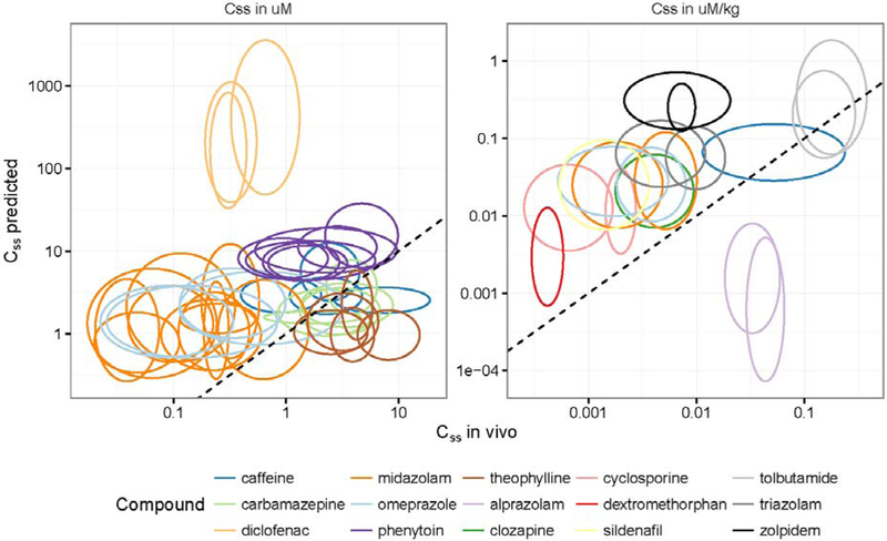
Comparisons of C_ss variability predicted using HTTK-Pop generated study populations averaged over 20 trials to in vivo C_ss variability (data collected in Johnson et al. 2006 [left panel] and Howgate et al. 2006 [right panel]). Each ellipse corresponds to a different in vivo study or pool of studies; each color corresponds to a chemical. For some chemicals, the results of multiple in vivo studies are included (represented by multiple ellipses in the same color). Ellipse centers are located at the median value in each dimension; ellipse axes encompass 95% confidence intervals on the observations in each dimension. The dashed line is the identity line. Ellipses centered at points on the identity line would indicate that the model predicted the same median C_ss as was observed in vivo. Perfect circles would indicate that the model predicted the same amount of variability in C_ss as was observed in vivo. Horizontally-elongated ellipses indicate that the model predicted less variability in C_ss than was observed in vivo; vertically-elongated ellipses indicate that the model predicted more variability in C_ss than was observed in vivo.

For the studies shown in the left-hand panel of Figure 3 (those compiled by Johnson et al. (2006)), HTTK-Pop predicts the range of the 95% CI within 2-fold of in vivo for 7/39 (18%); within 5-fold for 23/39 (59%); and within 10-fold for 28/39 (72%). For the studies shown in the right-hand panel of Figure 3 (compiled by Howgate et al. (2006)), HTTK-Pop predicts the range of the 95% CI within 2-fold of in vivo for 1/18 (6%); within 5-fold for 2/18 (11%); and within 10-fold for 7/18 (39%). Correlation between median model-predicted values and median in vivo values for these chemicals is also limited. The model of Johnson et al. (2006) predicted 90% of median clearance values within 2-fold of in vivo values; HTTK-Pop predicts only 8/39 (20%) of median C_ss values within 2-fold of in vivo values. HTTK-Pop predicts 24/39 values (62%) within 5-fold, and 30/39 values (77%) within 10-fold. Howgate et al. (2006) predicted median clearance within 2-fold of in vivo values for 73–78% of drugs. HTTK-Pop accomplishes the same only for 3/18 or 17%. HTTK-Pop predicts 7/18 values (39%) within 5-fold, and 10/18 values (56%) within 10-fold.

The log-transformed residuals for median C_ss were characterized, as well as the log-transformed residuals for the upper bound of the 95% CI (corresponding to 97.5^th percentile C_ss). They were tested for normality and summary statistics were computed. The results, shown in Table 5, indicated that the distribution of residuals was indeed non-normal for both data sets. Because arithmetic mean and median values are greater than 0, these results suggest that the model tends to over-predict both median and upper-bound C_ss.

Table 5.

Characterization of log-transformed residuals of median C_ss and 97.5^th percentile C_ss (upper bound on 95% CI) from Figure 3; variability factors from Figure 3, both in vivo and model-predicted; log-transformed residuals of variability factors from Figure 3. Distributions of all residuals were tested for normality by the Shapiro-Wilk test; all had p values < 1e-5, indicating statistically significant differences from normality.

For studies compiled by:	Howgate et al.				Johnson et al.
	Mean	Median	SD	95% interval	Mean	Median	SD	95% interval
Median Css residuals (log [predicted median Css /in vivo median Css])	1.21	1.61	1.95	−3.71−3.67	1.15	1.18	1.78	−1.68−5.50
97.5th %ile Css residuals (log [predicted 97.5th %ile Css /in vivo 97.5th %ile Css])	1.74	2.36	1.88	−2.65−4.06	1.38	1.12	2.23	−1.75−7.87
In vivo variability factor (in vivo 97.5th %ile Css /in vivo median Css)	2.28	2.10	0.78	1.33−4.55	2.52	2.25	0.97	1.36−5.41
Predicted variability factor (predicted 97.5th %ile Css /predicted median Css)	4.71	3.35	10.96	2.22−9.27	10.58	2.58	94.22	1.24−22.40
Variability factor residuals (log [predicted variability factor/in vivo variability factor])	0.53	0.50	0.57	−0.49−1.74	0.22	0.05	0.85	−0.84−2.45

The ratio of upper-bound C_ss to median C_ss was calculated for each study, for both predicted and in-vivo-derived values. This ratio can be interpreted as a variability factor; the larger it is, the greater the difference between median and upper-bound C_ss, indicating greater variability in C_ss and therefore individuals with greater sensitivity. Summary statistics were computed for this ratio for both predicted and in-vivo-derived values (Table 5). Then, the log-transformed residuals of this ratio were calculated, tested for normality, and summary statistics calculated. These results are also shown in Table 5. Again, these results suggest that the residuals are non-normal and that the model tends to over-predict the variability factor.

The results of a global sensitivity analysis of Equation 1 (presented in detail in the Supplemental Material, Section S2.2) indicated that variability in model-predicted C_ss is primarily driven by variability in either F_up or CL_int, depending on the chemical. Variability in the physiological parameters became important only for chemicals with low in vitro-measured intrinsic clearance (less than about 0.01 μL/min/million cells). The contributions of variability in each individual physiological parameter could not be separated, because the HTTK-Pop-simulated physiological parameters are not independently distributed. However, we also performed an exploratory sensitivity analysis in which the physiological parameters were assumed to be independently distributed, in which we could separately assess sensitivity of C_ss to each physiological parameter. In this analysis, we observed that for chemicals with low measured intrinsic clearance, variability in GFR became an important driver of variability in C_ss. These results indicate that variability in C_ss is primarily driven by variability in clearance rate for the primary clearance route for each chemical (hepatic or renal).

3.2. Comparing oral equivalent doses to exposures inferred from NHANES biomonitoring data

The model evaluation demonstrated that some large uncertainties remain, but that the errors tend to over-predict C_ss, which is a conservative bias for AER-based chemical risk prioritization (Wetmore et al. 2015). The predictive performance of HTTK-Pop for median C_ss is consistent with previous methods (Wambaugh et al. 2015). Predictions of variability in C_ss was not assessed by these previous methods and the previous HTTK method for simulating variability contained only a simple, body weight-based correlation structure (Wambaugh et al. 2015). Here we have gained the ability to use modern demographic information from the NHANES cohort to address human variability and establish sensitive populations. Therefore, we used HTTK-Pop to calculate demographic-specific AERs for the 50 chemicals (parent compounds only) with all necessary data (enumerated in Table 4).

AERs for the Total population are visualized as the comparison of OEDs and exposure estimates in Figure 4. Ranking chemicals by AER is intended to provide an approximate chemical risk prioritization. An AER less than or equal to 1 implies that the estimated exposure is greater than or equal to the dose needed to induce bioactivity. AER is less than 1 for only two chemicals (2,4-d, AER ≈ 0.09, and naphthalene, AER ≈ 0.5). AER increases quickly as one moves down the chemical ranking: triclosan has AER ≈ 8, and fenitrothion, AER ≈ 104. Despite the sometimes-wide ranges of OED and inferred median exposures (up to 6 orders of magnitude), the AER-based prioritization is able to characterize whether even the highest potential median exposure (upper confidence limit) is high enough to induce bioactivity. If there is 95% confidence that the exposure is well below the lowest OED, the breadth of the confidence interval may be irrelevant.

Figure 4.

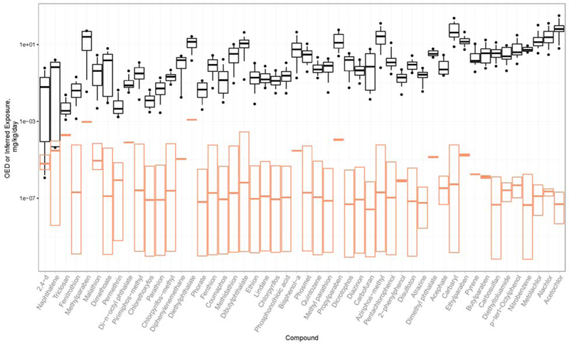
Black box-and-whisker plots show the range of oral equivalent doses over a range of ToxCast AC₅₀ percentiles, for the 95^th percentile C_ss in the Total population. Black bars indicate oral equivalent dose corresponding the median AC₅₀. Boxes range from 25^th percentile AC₅₀ to 75^th percentile AC₅₀ equivalent doses. Whiskers range from 10^th percentile AC₅₀ to 90^th percentile AC₅₀ equivalent doses. Filled circles indicate 5^th and 95^th percentile AC₅₀ equivalent doses. Orange box plots show the range of the 95% confidence interval on median exposures inferred from NHANES biomonitoring data: bars indicate the median exposure. The distance between the lower black whisker (corresponding to the 10^th percentile AC₅₀ equivalent dose) and the upper edge of the orange box, on a log scale, is the AER. (Note: For reasons of space, O-ethyl o-(p-nitrophenyl) phenylphosphonothioate is denoted by the shorter name Phosphonothioic acid, and 4-(1,1,3,3-tetramethylbutyl)phenol is denoted by the shorter name p-tert-Octylphenol.)

The C_ss values generated by HTTK-Pop and used to calculate OED for the Total population in Figure 4 were 13% higher (median) across the fifty chemicals than what had been previously calculated by Wambaugh et al. (2015). This resulted in a slight (12%) reduction of the OED for the Total population. For an individual chemical, the greatest increase in C_ss was 59% (for Fipronil). As shown in Table 5, the residual (unexplained) variability factor characterizing the sensitivity of the 95^th percentile ranges from 0.05 to 0.5; therefore, even small changes in the AER may be significant.

In Figure 5, we investigated how AER changes for the upper 95^th percentile of various demographic groups. AERs for the 50 chemicals were computed for all ten groups, and AERs for each group were compared to AERs for the Total population. For most chemicals, AERs are higher (lesser risk) for younger and non-obese populations; AERs are lower (greater risk) for ages above 65 or BMI above 30. All four paraben chemicals (fragrance preservatives) had relatively higher risk for women and reproductive-aged women.

Figure 5.

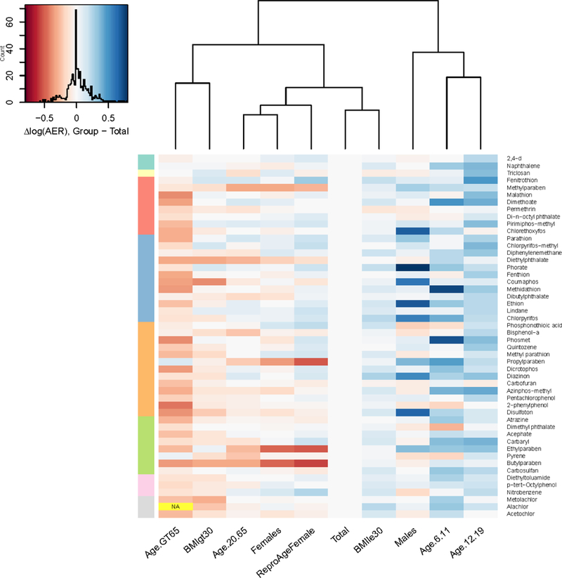
Difference in log₁₀ AER (number of orders of magnitude difference) between each demographic subgroup and the Total population. Chemicals are arranged from top to bottom in the same order as in Figure 4 (increasing AER for total population). Color bar at left indicates order of magnitude of AER in the Total population (from top to bottom: <=1, 100, 1 000, 10 000, etc.; no AERs on the order of 10 were observed in the Total population). The color of each cell represents the difference in log₁₀ AER from the Total population for the corresponding chemical (see color map with histogram, at top left). Red indicates lower AER (OED and exposure closer together); blue indicates higher AER (OED and exposure farther apart). (For reasons of space, O-ethyl o-(p-nitrophenyl) phenylphosphonothioate is denoted by the shorter name Phosphonothioic acid, and 4-(1,1,3,3-tetramethylbutyl)phenol is denoted by the shorter name p-tert-Octylphenol.)

In general, AER-based prioritization (relative ranking by AER) for the 50 chemicals is similar for all ten demographic groups considered in this analysis. AERs are at most about six times greater or lesser than for the total population. A six-fold change is relatively small compared to the order of magnitude of AERs for most chemicals in this set; all but three chemicals in Figure 4 had an AER greater than two orders of magnitude. Further, as shown in the comparison to actual in-vivo-measured variability (Table 5), the median unexplained difference between the median and 95^th percentile individuals in the available evaluation data sets (Figure 3) was roughly three-fold. However, in AER-based risk screening, AER is compared to an absolute threshold value; the changes in AER between demographic groups could result in different risk screening results for each group. (See Supplemental Material, Section S2.3.)

Because AER is the ratio of OED to exposure, the observed AER differences between groups may be induced either by differences in OED (i.e., by the inclusion of physiological variability in the reverse TK model), or by differences in exposure, or both. To elucidate the sources of the observed AER differences, we examined the differences in OED and exposure between each group and the Total population (Figure 6 and Figure 7). Throughout Figures 6–8, blue corresponds to higher AER (lesser risk) and red corresponds to lower AER (higher risk). Note that the color map is reversed for the exposure heatmap: lower exposures are colored in blue and higher exposures in red. Note also that the color map for all three plots is on the same scale (−0.8 to 0.8). For the groups Males, Females, and Reproductive-Age Females, relative to the Total population, chemicals (e.g., the parabens for women) with a large difference in AER have a large difference in exposure, but not a large difference in OED. These results imply that for these groups, the predicted differences in AER are mainly driven by differences in exposure. For the groups BMI GT 30 (obese individuals) and Age GT 65, AER is decreased for most chemicals relative to the Total population, exposure is slightly lower or unchanged, and OED is decreased. These results imply that for these groups, the decrease in AER is primarily driven by the decrease in OED, not by an increase in exposure.

Figure 6.

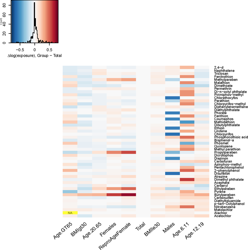
Difference in log₁₀ upper 95% confidence limit on median exposure between each demographic subgroup and the total population, for each chemical in the NHANES biomonitoring inference data set. Note that chemicals are arranged from top to bottom in the same order as Figure 6 (increasing AER).

Figure 7.

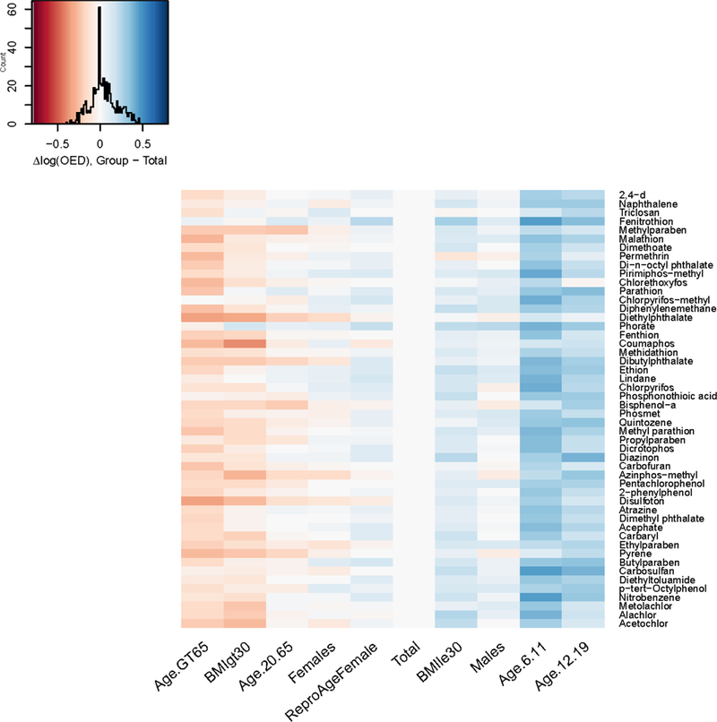
Difference in log₁₀ OED between each demographic subgroup and the total population, for each chemical in the NHANES biomonitoring inference data set. Note that chemicals are arranged from top to bottom in the same order as in Figure 6 (increasing AER).

By more accurately simulating variability in the OED, HTTK-Pop identified that the median C_ss was 73% higher for individuals aged greater than 65 than previously calculated for the total population (Wambaugh et al. 2015) and 49% greater for obese individuals. These increases lowered the OED by 42% and 33%, respectively. The combination of specific chemical and demographic group with the greatest change relative to the previous method was PCB136, which was 267% higher for the population aged greater than 65, corresponding to an OED decrease of 73%.

For the groups Age 6–11, Age 12–19, and BMI LE 30 (non-obese individuals), AER is increased (lesser risk) for most chemicals relative to the Total population, and the increase in AER appears to be mainly driven by an increase in OED, rather than by a decrease in exposure. In fact, for Age 6–11, exposure is markedly increased (i.e., indicating lesser risk) for many chemicals compared to the Total population, implying that the increase in OED outweighs the increase in exposure for these subgroups.

We note that, because of the assumed log-normal distribution of chemical exposure rates assumed by Wambaugh et al. (2014), the upper bounds on the 95% CI on the median exposures (plotted in Figure 5) depend upon both the central tendency and the estimated breadth of the distribution. For smaller data sets (e.g., males or females alone vs. the total population), there is greater uncertainty about the shape of the distribution. This contributes to some of the observed differences in upper-bound inferred exposures (Wambaugh et al. 2014).

We also note that uncertainty in model-predicted OED (over- or under-estimation) contributes uncertainty to AER-based relative ranking. However, the error in model-predicted OED is likely to be in the same direction across demographic groups for a given chemical. Thus, HTTK-Pop may be useful to identify populations more or less sensitive to a given chemical.

Although the chemical-specific changes in the AER for the 50 chemicals analyzed here are at most six-fold, there are clear implications for the identification of sensitive populations among the modern U.S. demographic groups. In particular, the reduced clearance of adults aged greater than 65 makes them generally one of the most sensitive populations. Meanwhile, the enhanced clearance of younger life-stages (per kg body weight) on average increases the margin between exposure and putative bioactive dose, indicating lesser risk despite the higher exposure rates of younger life stages.

4. Discussion

We incorporated physiological variability based on recent data from a large-scale survey of the U.S. population (NHANES) into HTTK-Pop, a high throughput toxicokinetic modeling tool. This model extends an existing open-source high-throughput toxicokinetic (TK) framework (Pearce et al. 2016). Using HTTK-Pop, we evaluated predictions of plasma concentration by comparison to values derived from in vivo measurements for 95 compounds (Obach et al. 2008; Wetmore et al. 2012). We also evaluated predictions of inter-individual variability by comparison to in vivo measurements in 14 compounds (Howgate et al. 2006; Johnson et al. 2006). Finally, we simulated ten demographic groups within the modern, U.S. population. In each demographic group, we performed reverse TK on ToxCast high throughput screening (HTS) data to predict the population distributions of the oral equivalent doses (OEDs) for each of fifty chemicals with exposures indicated by NHANES urine biomonitoring data (Wambaugh et al. 2014). Although, to date, HTS data itself does not incorporate variability between demographic groups, we can now include this variability for both TK and exposure.

Chemical AERs for each demographic group were compared to the corresponding AERs in the total population (Section 3.5). We identified chemicals and demographic groups with the smallest margin between OED and exposure (i.e., the activity:exposure ratio or AER). This analysis found that AERs were consistently higher (lower risk) across chemicals for children ages 6–11, adolescents ages 12–19, and non-obese people. This result occurs because the OEDs tend to be higher for these populations than for the total population (see Figure 7 and Supplemental Material Section S3.2). Thus, a fixed 1 mg/kg/day dose results in a consistently lower 95^th percentile steady-state plasma concentration, and therefore a consistently higher OED. However, we did find that the population aged greater than 65 had lower AERs (higher risk). We further found that for women, and especially reproductive aged women, that AERs for paraben chemicals were lower. However, for the fifty chemicals examined the relative change in the AERs is less than one order of magnitude in all cases, indicating that the priority of these chemicals relative to each other would not have changed. For any one chemical, the predictive error will be similar across demographic groups, so that the relative ranking between demographic groups may be more certain.

HTTK-Pop predicts higher OEDs in children ages 6–11 compared to the overall population (Figure 7), equivalent to higher predicted total clearance in this age range. This prediction is consistent with in vivo PK data compiled from studies on 45 chemicals (all pharmaceuticals) in children, adolescents, and adults (Ginsberg et al. 2002). Ginsberg et al. (2002) found that, across 27 chemicals with in vivo clearance data, children ages 2–12 years had significantly higher clearance per kg body weight than adults. The increased clearance in children is attributed by Ginsberg et al. (2003) to a combination of isozyme ontogeny and physiology. Where data exist, isozyme abundances and activities reach near-adult levels by approximately age 1, so that the intrinsic clearance rate is approximately equal in children and adults (Ginsberg et al. 2003). These data on isozyme ontogeny support HTTK-Pop’s use of CL_int values based on measurements in adult hepatocytes for the age groups simulated in this report. Furthermore, children tend to have larger livers and greater blood flow for their bodyweight than adults have (Ginsberg et al. 2003), which combine with the near-adult intrinsic clearance rate to produce a higher total clearance rate per kg bodyweight. HTTK-Pop reflects these differences in liver size and blood flow in the simulated populations of children and adolescents (Supplemental Material: Section S3.2).

The lower AERs (higher risk) noted for the population aged greater than 65 can also be linked to physiologic differences that manifest during this life stage, resulting in lower OEDs. Supporting evidence for this observation can be found in a TK meta-analysis assessing trends in clearance across adults aged 18 to over 85 years across over 46 compounds (Ginsberg et al., 2005). This study showed a concomitant decrease in clearance with increasing age, with steeper decreases observed for individuals aged over 60 years. These decreases have been attributed to decreases in tissue blood flow rates, glomerular filtration rates, and hepatic clearance, the latter of which is impacted by decreased liver size, cytochrome P450 enzyme content, bile flow, and blood flow (Ginsberg et al., 2005). HTTK-Pop reflects these differences in liver size, liver blood flow, and GFR (Supplemental Material: Section S2.7).

The variability simulation approach used here was developed taking into consideration previous population physiology simulations, including P3M (Price 2003), PK-Pop (Willmann et al. 2007), physB (Bosgra et al. 2012), SimCyp (Jamei et al. 2009a; Jamei et al. 2009b), and especially PopGen (McNally et al. 2014). However, HTTK-Pop has notable improvements over these software packages. First, HTTK-Pop can generate simulated populations by either 1) direct resampling of its reference database, or 2) use of a virtual-individuals method that is based on interpolation of the reference database. Second, in the virtual-individuals mode, HTTK-Pop takes a more detailed approach to reproducing the correlation structure of its reference database than does previous software. Other population physiology simulators that generate virtual individuals tend to approximate the population age distribution using parametric or piecewise linear distributions, and distributions of age-dependent height and weight using piecewise polynomial approximations with normally distributed residual variability (Howgate et al. 2006; Johnson et al. 2006; McNally et al. 2014; Willmann et al. 2007). By contrast, HTTK-Pop uses gender- and ethnicity-specific non-parametric distributions to model age, height, and weight. Finally, HTTK-Pop uses the most recent publicly available NHANES data as a reference database. Both P3M and PopGen use NHANES III (1988–1994) as a reference database, and thus may not accurately reproduce demographic and anthropometric quantities that have changed in the U.S. population over the last 20 years. HTTK-Pop is specifically designed to produce better and more representative U.S. populations and subpopulations.

Simulating NHANES individuals had limited ability to reproduce variability in C_ss observed in vivo (Section 3.1). An important source of the disagreement may involve HTTK-Pop’s assumptions about the distributions of the chemical-specific parameters F_up and CL_int. Global sensitivity analysis (Supplemental Material S2.4) indicated that C_ss is primarily sensitive to either F_up or CL_int, depending on the chemical. Thus, assumptions made about the distributions of these parameters may have a strong influence on the model results.

The distributions assumed by HTTK-Pop are idealized approximations that can be revised only after more data become available. This is particularly true of chemical-specific HTTK data for in vitro measured unbound fraction in plasma (F_up) and hepatic metabolism (CL_int). The distribution of F_up depends on inter-individual variability in plasma protein concentrations, particularly for the two plasma proteins responsible for most chemical/drug binding, albumin and alpha-1-acid glycoprotein (AAG) (Routledge 1986). AAG binding may be particularly important for basic compounds (Israili and Dayton 2001; Routledge 1986). Plasma lipoprotein concentrations may also affect the unbound fraction in plasma, particularly for lipophilic compounds that tend to associate with lipoproteins (Wasan et al. 2008). Data are available for inter-individual variability in these plasma protein concentrations: NHANES measured serum albumin concentrations and blood lipids in respondents ages 12–80, providing information on correlation of these concentration with the other NHANES demographic, anthropometric, and laboratory quantities (Johnson et al. 2014). Several studies have quantified correlations of AAG concentrations with age, ethnicity, gender, and disease state (summarized in Israili and Dayton 2001). Improving accuracy in predicting inter-individual variability in F_up will require substance-specific relative affinities for albumin, AAG, and lipoproteins, which cannot be estimated from the in vitro measurements of F_up in pooled plasma samples that are currently available for these chemicals. A high-throughput method to measure or predict these binding affinities would improve HTTK-Pop’s ability to simulate inter-individual variability in F_up. The distribution of F_up may also depend on inter-individual variability in plasma lipids, particularly for lipophilic compounds.

The distributions assumed for CL_int could also be refined with more data. Sources of inter-individual variability in CL_int include variability in the abundance and phenotype of each hepatic isozyme that metabolizes a given compound, which are known to be correlated with demographic factors (Barter et al. 2007; Barter et al. 2008; Hines 2007; Kedderis and Lipscomb 2001; Yasuda et al. 2008; Yeo et al. 2004). CV of abundance has been estimated at 31% for CYP3A4 and 36% for CYP2E1 (Lipscomb et al. 2003). CV of isozyme-specific CL_int has been estimated at 33% for CYP3A4 (Kato et al. 2010); 60–70% for CYP2D6 (Chiba et al. 2012); 66% in extensive CYP2C19 metabolizers, and 26% in poor CYP2C19 metabolizers (Chiba et al. 2014). HTTK-Pop’s assumption of 30% CV in overall CL_int may therefore be reasonable for compounds primarily metabolized by CYP3A4 or 2E1, but may be an underestimate for compounds primarily metabolized by CYP2D6 or 2C19. Furthermore, the true prevalence of PMs is isozyme-specific and varies with ethnicity. HTTK-Pop’s assumption of 5% PMs is within the estimated range of the proportion of CYP 2C19, 2C9, and 2D6 PMs based on data on ethnicity-specific proportions of CYP-specific PMs, combined with NHANES data on the proportion of each ethnicity in the US population (Belle and Singh 2008; Bernard et al. 2006; Hiratsuka 2012; Inoue et al. 2006; Luo et al. 2006; Mizutani 2003; Strom et al. 2011). (More details on the source data used for this estimation is available in Supplemental Material Section S3.1.) Approximating inter-individual variability in overall Cl_int can be done more accurately using an isozyme-specific IVIVE approach, combining in vitro measurements of isozyme-specific intrinsic clearance rates for each chemical with information on age- and ethnicity-specific prevalence of various isozymes, proportion of PMs, and residual variability (Cubitt et al. 2011).

For environmental chemicals, isozyme-specific clearance data are not typically gathered. Isozyme-specific data allows very accurate predictions of inter-individual variability in steady-state clearance. The compounds considered by Johnson et al. and Howgate et al. were selected because they had adequate published in vitro data on CYP-specific metabolism to allow an isozyme-specific IVIVE approach to estimating clearance (Howgate et al. 2006; Johnson et al. 2006). The models in these publications therefore perform significantly better than HTTK-Pop, because they include isozyme-specific clearance estimation while HTTK-Pop does not. While isozyme-specific intrinsic clearance has been measured for a few environmental compounds using recombinant CYPs (Wetmore et al. 2014), this method is currently not feasible for screening large numbers of chemicals. HTTK-Pop’s simulation of inter-individual variability in CL_int would be improved by a reliable high-throughput method to measure or predict isozyme-specific clearance.

Direct in vitro high-throughput screening of inter-individual variability in plasma protein binding or hepatic metabolism is not yet available; such techniques would require plasma samples or hepatocytes from large numbers of individuals. The Thousand Genomes High-Throughput Screening Survey has performed such in vitro high-throughput screening for inter-individual variability in cytotoxic responses, using lymphoblastoid cell lines (Abdo et al. 2015); however, such techniques have not yet been developed to screen for inter-individual variability in metabolism or plasma protein binding. Therefore, our suggestions above focus on estimating inter-individual variability by combining in vitro measurements of average or median plasma protein binding or isozyme-specific metabolism with information on inter-individual variability in plasma protein concentrations or isozyme abundance and activity.

5. Conclusion

Our work has improved high throughput risk prioritization for large numbers of environmental chemicals by adding simulated inter-individual TK variability that describes the modern U.S. population.

We have developed HTTK-Pop, a method that uses the CDC NHANES anthropometric data to simulate the appropriate correlation structure for physiological parameters relevant to TK. As an example, in vitro bioactivities (μM concentrations) identified from HTS data were converted to oral equivalent dose rates (mg/kg/day) for different demographic groups. Oral equivalent dose estimates were then compared with estimated exposure rates for the corresponding groups, yielding estimates of the margin between environmental exposure rates and dose rates that might pose a hazard for fifty chemicals across ten demographic groups within the U.S. population. We identified demographic groups and life stages that are potentially more sensitive to exposure to various environmental chemicals. This open-source model provides transparency for review, allows modification of the underlying models as needed to support decision making, and can be expanded as new data become available.

Table 3.

HTTK-Pop specifications by demographic group

Demographic group	Specifications for HTTK-Pop	Number of females among 1000 simulated individuals
Total	None (all ages, sexes, races/ethnicities, and weight classes included)	496
Ages 6–11	Age limits 6 – 11 years	462
Ages 12–19	Age limits 12 – 19 years	491
Ages 20–65	Age limits 20 −65 years	519
Ages > 65	Age limits 66 – 79 years	541
BMI <= 30	Weight classes Underweight, Normal, and Overweight	491
BMI > 30	Weight class Obese	497
Males	Number of males = 1000; number of females = 0	0
Females	Number of females = 1000; number of males = 0	1000
Reproductive Age Females	Number of females = 1000; number of males = 0	1000
	Age limits 16 – 49 years

References

- Abdo N; Xia M; Brown CC; Kosyk O; Huang R; Sakamuru S, et al. Population-based in vitro hazard and concentration-response assessment of chemicals: the 1000 Genomes high-throughput screening Study. Environmental Health Perspectives 2015;123:458. [DOI] [PMC free article] [PubMed] [Google Scholar]
- Aylward LL; Hays SM Consideration of dosimetry in evaluation of ToxCast™ data. Journal of Applied Toxicology 2011;31:741–751 [DOI] [PubMed] [Google Scholar]
- Barter ZE; Bayliss MK; Beaune PH; Boobis AR; Carlile DJ; Edwards RJ, et al. Scaling factors for the extrapolation of in vivo metabolic drug clearance from in vitro data: reaching a consensus on values of human micro-somal protein and hepatocellularity per gram of liver. Current Drug Metabolism 2007;8:33–45 [DOI] [PubMed] [Google Scholar]
- Barter ZE; Chowdry JE; Harlow JR; Snawder JE; Lipscomb JC; Rostami-Hodjegan A Covariation of human microsomal protein per gram of liver with age: absence of influence of operator and sample storage may justify interlaboratory data pooling. Drug Metabolism and Disposition 2008;36:2405–2409 [DOI] [PubMed] [Google Scholar]
- Baxter‐Jones AD; Faulkner RA; Forwood MR; Mirwald RL; Bailey DA Bone Mineral Accrual from 8 to 30 Years of Age: An Estimation of Peak Bone Mass. Journal of Bone and Mineral Research 2011;26:1729–1739 [DOI] [PubMed] [Google Scholar]
- Belle DJ; Singh H. Genetic factors in drug metabolism. American Family Physician 2008;77 [PubMed] [Google Scholar]
- Bernard S; Neville KA; Nguyen AT; Flockhart DA Interethnic differences in genetic polymorphisms of CYP2D6 in the US population: clinical implications. The Oncologist 2006;11:126–135 [DOI] [PubMed] [Google Scholar]
- Birnbaum L; Bischoff K; Blancato J; Clewell H; Dedrick R; Delp M, et al. Physiological Parameter Values for PBPK Models. International Life Sciences Institute Risk Sciences Institute; 1994 [Google Scholar]
- Bosgra S; van Eijkeren J; Bos P; Zeilmaker M; Slob W An improved model to predict physiologically based model parameters and their inter-individual variability from anthropometry. Critical Reviews in Toxicology 2012;42:751–767 [DOI] [PubMed] [Google Scholar]
- Chiba K; Kato M; Ito T; Suwa T; Sugiyama Y Inter-individual variability of in vivo CYP2D6 activity in different genotypes. Drug Metabolism and Pharmacokinetics 2012;27:405–413 [DOI] [PubMed] [Google Scholar]
- Chiba K; Shimizu K; Kato M; Nishibayashi T; Terada K; Izumo N, et al. Prediction of inter-individual variability in the pharmacokinetics of CYP2C19 substrates in humans. Drug Metabolism and Pharmacokinetics 2014;29:379–386 [DOI] [PubMed] [Google Scholar]
- Cubitt HE; Rowland-Yeo K; Howgate EM; Rostami-Hodjegan A; Barter ZE Sources of interindividual variability in IVIVE of clearance: an investigation into the prediction of benzodiazepine clearance using a mechanistic population-based pharmacokinetic model. Xenobiotica 2011;41:623–638 [DOI] [PubMed] [Google Scholar]
- Ginsberg G; Hattis D; Sonawane B; Russ A; Banati P; Kozlak M, et al. Evaluation of child/adult pharmacokinetic differences from a database derived from the therapeutic drug literature. Toxicological Sciences 2002;66:185–200 [DOI] [PubMed] [Google Scholar]
- Ginsberg G; Slikker W; Bruckner J; Sonawane B Incorporating Children’s Toxicokinetics into a Risk Framework. Environmental Health Perspectives 2003;112:272–283 [DOI] [PMC free article] [PubMed] [Google Scholar]
- Glen G; Isaacs K Estimating Sobol sensitivity indices using correlations. Environmental Modelling & Software 2012;37:157–166 [Google Scholar]
- Grummer-Strawn LM; Reinold CM; Krebs NF; Control C.f.D.; Prevention. Use of World Health Organization and CDC growth charts for children aged 0–59 months in the United States. Department of Health and Human Services, Centers for Disease Control and Prevention; 2010 [PubMed] [Google Scholar]
- Haycock GB; Schwartz GJ; Wisotsky DH Geometric method for measuring body surface area: a height-weight formula validated in infants, children, and adults. The Journal of Pediatrics 1978;93:62–66 [DOI] [PubMed] [Google Scholar]
- Hines RN Ontogeny of human hepatic cytochromes P450. Journal of Biochemical and Molecular Toxicology 2007;21:169–175 [DOI] [PubMed] [Google Scholar]
- Hiratsuka M In vitro assessment of the allelic variants of cytochrome P450. Drug Metabolism and Pharmacokinetics 2012;27:68–84 [DOI] [PubMed] [Google Scholar]
- Howgate E; Rowland-Yeo K; Proctor N; Tucker G; Rostami-Hodjegan A Prediction of in vivo drug clearance from in vitro data. I: impact of inter-individual variability. Xenobiotica 2006;36:473–497 [DOI] [PubMed] [Google Scholar]
- Inoue S; Howgate E; Rowland-Yeo K; Shimada T; Yamazaki H; Tucker G, et al. Prediction of in vivo drug clearance from in vitro data. II: Potential inter-ethnic differences. Xenobiotica 2006;36:499–513 [DOI] [PubMed] [Google Scholar]
- Israili Z; Dayton P Human Alpha-1-Glycoprotein and its Interations with Drugs. Drug Metabolism Reviews 2001;33:161–235 [DOI] [PubMed] [Google Scholar]
- Jacques J; Lavergne C; Devictor N Sensitivity analysis in presence of model uncertainty and correlated inputs. Reliability Engineering & System Safety 2006;91:1126–1134 [Google Scholar]
- Jamei M; Dickinson GL; Rostami-Hodjegan A A framework for assessing inter-individual variability in pharmacokinetics using virtual human populations and integrating general knowledge of physical chemistry, biology, anatomy, physiology and genetics: a tale of ‘bottom-up’vs ‘top-down’recognition of covariates. Drug Metabolism and Pharmacokinetics 2009a;24:53–75 [DOI] [PubMed] [Google Scholar]
- Jamei M; Marciniak S; Feng K; Barnett A; Tucker G; Rostami-Hodjegan A The Simcyp® population-based ADME simulator. Expert Opinion on Drug Metabolism & Toxicology 2009b;5:211–223 [DOI] [PubMed] [Google Scholar]
- Johnson CL; Dohrmann SM; Burt VL; Mohadjer LK National health and nutrition examination survey: sample design, 2011–2014. Vital and Health Statistics Series 2, Data Evaluation and Methods Research 2014:1–33 [PubMed] [Google Scholar]
- Johnson CL; Paulose-Ram R; Ogden CL; Carroll MD; Kruszon-Moran D; Dohrmann SM, et al. National health and nutrition examination survey: analytic guidelines, 1999–2010. Vital and Health Statistics Series 2, Data Evaluation and Methods Research 2013:1–24 [PubMed] [Google Scholar]
- Johnson TN; Rostami-Hodjegan A; Tucker GT Prediction of the clearance of eleven drugs and associated variability in neonates, infants and children. Clinical Pharmacokinetics 2006;45:931–956 [DOI] [PubMed] [Google Scholar]
- Judson RS; Kavlock RJ; Setzer RW; Cohen Hubal EA; Martin MT; Knudsen TB, et al. Estimating toxicity-related biological pathway altering doses for high-throughput chemical risk assessment. Chemical Research in Toxicology 2011;24:451–462 [DOI] [PubMed] [Google Scholar]
- Kato M; Chiba K; Ito T; Koue T; Sugiyama Y Prediction of interindividual variability in pharmacokinetics for CYP3A4 substrates in humans. Drug Metabolism and Pharmacokinetics 2010;25:367–378 [DOI] [PubMed] [Google Scholar]
- Kavlock R; Chandler K; Houck K; Hunter S; Judson R; Kleinstreuer N, et al. Update on EPA’s ToxCast program: providing high throughput decision support tools for chemical risk management. Chemical Research in Toxicology 2012;25:1287–1302 [DOI] [PubMed] [Google Scholar]
- Kedderis GL; Lipscomb JC Application of in vitro biotransformation data and pharmacokinetic modeling to risk assessment. Toxicology and Industrial Health 2001;17:315–321 [DOI] [PubMed] [Google Scholar]
- Koo WW; Walters JC; Hockman EM Body composition in human infants at birth and postnatally. The Journal of Nutrition 2000;130:2188–2194 [DOI] [PubMed] [Google Scholar]
- Kuczmarski RJ; Ogden CL; Guo SS; Grummer-Strawn LM; Flegal KM; Mei Z, et al. 2000 CDC Growth Charts for the United States: methods and development. Vital and Health Statistics Series 11, Data from the National Health Survey 2002:1 [PubMed] [Google Scholar]
- Levey AS; Stevens LA; Schmid CH; Zhang YL; Castro AF; Feldman HI, et al. A new equation to estimate glomerular filtration rate. Annals of Internal Medicine 2009;150:604–612 [DOI] [PMC free article] [PubMed] [Google Scholar]
- Lipscomb JC; Kedderis GL Incorporating human interindividual biotransformation variance in health risk assessment. Science of the Total Environment 2002;288:13–21 [DOI] [PubMed] [Google Scholar]
- Lipscomb JC; Teuschler LK; Swartout JC; Striley CA; Snawder JE Variance of microsomal protein and cytochrome P450 2E1 and 3A forms in adult human liver. Toxicology Mechanisms and Methods 2003;13:45–51 [DOI] [PubMed] [Google Scholar]
- Looker A; Borrud L; Hughes J; Fan B; Shepherd J; Sherman M Total body bone area, bone mineral content, and bone mineral density for individuals aged 8 years and over: United States, 1999–2006. Vital and Health Statistics Series 11, Data from the National Health Survey 2013:1–78 [PubMed] [Google Scholar]
- Lubin B Reference values in infancy and childhood in: Nathan D, Oski F, eds. Hematology of Infancy and Childhood; 1987 [Google Scholar]
- Lumley T Analysis of complex survey samples. Journal of Statistical Software 2004;9:1–19 [Google Scholar]
- Luo HR; Poland RE; Lin KM; Wan YJY Genetic polymorphism of cytochrome P450 2C19 in Mexican Americans: A cross‐ethnic comparative study. Clinical Pharmacology & Therapeutics 2006;80:33–40 [DOI] [PubMed] [Google Scholar]
- Ma MK; Woo MH; Mcleod HL Genetic basis of drug metabolism. American Journal of Health System Pharmacy 2002;59:2061–2069 [DOI] [PubMed] [Google Scholar]
- McNally K; Cotton R; Hogg A; Loizou G PopGen: a virtual human population generator. Toxicology 2014;315:70–85 [DOI] [PubMed] [Google Scholar]
- Mizutani T PM frequencies of major CYPs in Asians and Caucasians. Drug Metabolism Reviews 2003;35:99–106 [DOI] [PubMed] [Google Scholar]
- Obach RS; Lombardo F; Waters NJ Trend analysis of a database of intravenous pharmacokinetic parameters in humans for 670 drug compounds. Drug Metabolism and Disposition 2008;36:1385–1405 [DOI] [PubMed] [Google Scholar]
- Ogden CL; Carroll MD; Kit BK; Flegal KM Prevalence of childhood and adult obesity in the United States, 2011–2012. JAMA 2014;311:806–814 [DOI] [PMC free article] [PubMed] [Google Scholar]
- Ogiu N; Nakamura Y; Ijiri I; Hiraiwa K; Ogiu T A statistical analysis of the internal organ weights of normal Japanese people. Health Physics 1997;72:368–383 [DOI] [PubMed] [Google Scholar]
- Park YH; Lee K; Soltow QA; Strobel FH; Brigham KL; Parker RE, et al. High-performance metabolic profiling of plasma from seven mammalian species for simultaneous environmental chemical surveillance and bioeffect monitoring. Toxicology 2012;295:47–55 [DOI] [PMC free article] [PubMed] [Google Scholar]
- Pearce R; Strope C; Setzer RW; Sipes N; Wambaugh JF httk: R Package for High-Throughput Toxicokinetics. Journal of Statistical Software 2016:in press [DOI] [PMC free article] [PubMed] [Google Scholar]
- Price, P. Instructions for Use of Software Physiological Parameters for PBPK Modeling Version 1.3 (P3MTM 1.3). 2003
- Price PS; Conolly RB; Chaisson CF; Gross EA; Young JS; Mathis ET, et al. Modeling interindividual variation in physiological factors used in PBPK models of humans. Critical Reviews in Toxicology 2003;33:469–503 [PubMed] [Google Scholar]
- Rager JE; Strynar MJ; Liang S; McMahen RL; Richard AM; Grulke CM, et al. Linking high resolution mass spectrometry data with exposure and toxicity forecasts to advance high-throughput environmental monitoring. Environment International 2016;88:269–280 [DOI] [PubMed] [Google Scholar]
- Rotroff DM; Wetmore BA; Dix DJ; Ferguson SS; Clewell HJ; Houck KA, et al. Incorporating human dosimetry and exposure into high-throughput in vitro toxicity screening. Toxicological Sciences 2010;117:348–358 [DOI] [PMC free article] [PubMed] [Google Scholar]
- Routledge P The plasma protein binding of basic drugs. British Journal of Clinical Pharmacology 1986;22:499–506 [DOI] [PMC free article] [PubMed] [Google Scholar]
- Saltelli A; Annoni P; Azzini I; Campolongo F; Ratto M; Tarantola S Variance based sensitivity analysis of model output. Design and estimator for the total sensitivity index. Computer Physics Communications 2010;181:259–270 [Google Scholar]
- Schmitt W General approach for the calculation of tissue to plasma partition coefficients. Toxicology in Vitro 2008;22:457–467 [DOI] [PubMed] [Google Scholar]
- Schwartz GJ; Work DF Measurement and estimation of GFR in children and adolescents. Clinical Journal of the American Society of Nephrology 2009;4:1832–1843 [DOI] [PubMed] [Google Scholar]
- Sohlenius-Sternbeck A-K; Afzelius L; Prusis P; Neelissen J; Hoogstraate J; Johansson J, et al. Evaluation of the human prediction of clearance from hepatocyte and microsome intrinsic clearance for 52 drug compounds. Xenobiotica 2010;40:637–649 [DOI] [PubMed] [Google Scholar]
- Strom CM; Goos D; Crossley B; Zhang K; Buller-Burkle A; Jarvis M, et al. Testing for variants in CYP2C19: population frequencies and testing experience in a clinical laboratory. Genetics in Medicine 2011;14:95–100 [DOI] [PubMed] [Google Scholar]
- Strope CL; Mansouri K; Kancherla J; Stevens C; Wambaugh JF High-Throughput Pharmacokinetic Modeling Using Computationally Predicted Parameter Values: Dissociation Constants Society of Toxicology Annual Meeting. San Diego, CA; 2015 [Google Scholar]
- Tan Y-M; Liao KH; Clewell HJ Reverse dosimetry: interpreting trihalomethanes biomonitoring data using physiologically based pharmacokinetic modeling. Journal of Exposure Science and Environmental Epidemiology 2007;17:591–603 [DOI] [PubMed] [Google Scholar]
- Tan Y-M; Liao KH; Conolly RB; Blount BC; Mason AM; Clewell HJ Use of a physiologically based pharmacokinetic model to identify exposures consistent with human biomonitoring data for chloroform. Journal of Toxicology and Environmental Health, Part A 2006;69:1727–1756 [DOI] [PubMed] [Google Scholar]
- Thomas RS; Philbert MA; Auerbach SS; Wetmore BA; Devito MJ; Cote I, et al. Incorporating new technologies into toxicity testing and risk assessment: moving from 21st century vision to a data-driven framework. Toxicological Sciences 2013;136:4–18 [DOI] [PMC free article] [PubMed] [Google Scholar]
- Tonnelier A; Coecke S; Zaldívar J-M Screening of chemicals for human bioaccumulative potential with a physiologically based toxicokinetic model. Archives of Toxicology 2012;86:393–403 [DOI] [PMC free article] [PubMed] [Google Scholar]
- USEPA. Integrated Bioactivity and Exposure Ranking: A Computational Approach for the Prioritization and Screening of Chemicals in the Endocrine Disruptor Screening Program. 2014
- USEPA. EPI (Estimation Programs Interface) Suite. 2015
- USGAO. Toxic Substances: EPA Has Increased Efforts to Assess and Control Chemicals but Could Strengthen Its Approach. in: Office U.S.G.A., ed; 2013 [Google Scholar]
- Valentin J Basic anatomical and physiological data for use in radiological protection: reference values: ICRP Publication 89. Annals of the ICRP 2002;32:1–277 [PubMed] [Google Scholar]
- Verbraecken J; Van de Heyning P; De Backer W; Van Gaal L Body surface area in normal-weight, overweight, and obese adults. A comparison study. Metabolism 2006;55:515–524 [DOI] [PubMed] [Google Scholar]
- Wambaugh JF; Setzer RW; Reif DM; Gangwal S; Mitchell-Blackwood J; Arnot JA, et al. High-throughput models for exposure-based chemical prioritization in the ExpoCast project. Environmental Science and Technology 2013;47:8479–8488 [DOI] [PubMed] [Google Scholar]
- Wambaugh JF; Wang A; Dionisio KL; Frame A; Egeghy P; Judson R, et al. High throughput heuristics for prioritizing human exposure to environmental chemicals. Environmental Science and Technology 2014;48:12760–12767 [DOI] [PubMed] [Google Scholar]
- Wambaugh JF; Wetmore BA; Pearce R; Strope C; Goldsmith R; Sluka JP, et al. Toxicokinetic Triage for Environmental Chemicals. Toxicological Sciences 2015;147:55–67 [DOI] [PMC free article] [PubMed] [Google Scholar]
- Webber CE; Barr RD Age‐and gender‐dependent values of skeletal muscle mass in healthy children and adolescents. Journal of Cachexia, Sarcopenia and Muscle 2012;3:25–29 [DOI] [PMC free article] [PubMed] [Google Scholar]
- Wetmore BA; Allen B; Clewell HJ 3rd; Parker T; Wambaugh JF; Almond LM, et al. Incorporating population variability and susceptible subpopulations into dosimetry for high-throughput toxicity testing. Toxicological Sciences 2014;142:210–224 [DOI] [PubMed] [Google Scholar]
- Wetmore BA; Wambaugh JF; Allen B; Ferguson SS; Sochaski MA; Setzer RW, et al. Incorporating High-Throughput Exposure Predictions With Dosimetry-Adjusted In Vitro Bioactivity to Inform Chemical Toxicity Testing. Toxicological Sciences 2015;148:121–136 [DOI] [PMC free article] [PubMed] [Google Scholar]
- Wetmore BA; Wambaugh JF; Ferguson SS; Sochaski MA; Rotroff DM; Freeman K, et al. Integration of dosimetry, exposure, and high-throughput screening data in chemical toxicity assessment. Toxicological Sciences 2012;125:157–174 [DOI] [PubMed] [Google Scholar]
- WHO. WHO child growth standards : length/height-for-age, weight-for-age, weight-for-length, weight-for-height and body mass index-for-age : methods and development. in: WHO D.o.N.f.H.a.D, ed; 2006 [Google Scholar]
- WHO. WHO Anthro for Personal Computers Manual: Software for assessing growth and development of the world’s children, version 3.2.2, 2011. in: (WHO) W.H.O., ed. Geneva: WHO; 2010 [Google Scholar]
- Wilkinson GR; Shand DG Commentary: a physiological approach to hepatic drug clearance. Clinical Pharmacology and Therapeutics 1975;18:377–390 [DOI] [PubMed] [Google Scholar]
- Willmann S; Höhn K; Edginton A; Sevestre M; Solodenko J; Weiss W, et al. Development of a physiology-based whole-body population model for assessing the influence of individual variability on the pharmacokinetics of drugs. Journal of Pharmacokinetics and Pharmacodynamics 2007;34:401–431 [DOI] [PubMed] [Google Scholar]
- Yasuda SU; Zhang L; Huang SM The role of ethnicity in variability in response to drugs: focus on clinical pharmacology studies. Clinical Pharmacology & Therapeutics 2008;84:417–423 [DOI] [PubMed] [Google Scholar]
- Yeo KR; Rostami-Hodjegan A; Tucker G Abundance of cytochromes P450 in human liver. British Journal of Clinical Pharmacology 2004;57:687–688 [Google Scholar]
Associated Data
This section collects any data citations, data availability statements, or supplementary materials included in this article.