Automatic Tuning of Virtual Constraint-Based Control Algorithms for Powered Knee-Ankle Prostheses

Abstract

State-of-art powered prosthetic legs are often controlled using a collection of joint impedance controllers designed for different phases of a walking cycle. Consequently, finite state machines are used to control transitions between different phases. This approach requires a large number of impedance parameters and switching rules to be tuned. Since one set of control parameters cannot be used across different amputees, clinicians spend enormous time tuning these gains for each patient. This paper proposes a virtual constraint-based control scheme with a smaller set of control parameters, which are automatically tuned in real-time using an extremum seeking controller (ESC). ESC, being a model-free control method, assumes no prior knowledge of either the prosthesis or human. Using a singular perturbation analysis, we prove that the virtual constraint tracking errors are small and the PD gains remain bounded. Simulations demonstrate that our ESC-based method is capable of adapting the virtual-constraint based control parameters for amputees with different masses.

I. INTRODUCTION

State-of-art powered prosthetic legs are often controlled using a predetermined collection of joint impedance controllers [1], [2] designed for different phases of a walking cycle. Finite state machines are, then, employed to control transitions between each two joint impedance control laws [3]–[5]. In this approach, a gait cycle is typically divided into multiple (usually 4 or 5) gait phases, where each phase has at least three joint impedance control parameters (stiffness, viscosity, and equilibrium angle) for each actuated joint. However, these parameters do not generalize across amputees due to physiological differences. The tuning process for each patient can take around four to five hours due to the large number of patient-specific parameters [6].

In order to reduce the burden of clinicians, approaches such as rule-based fuzzy logic inference [7], model-based methods [8], and cyber expert systems [9] have been used to automatically find an optimum set of parameters for prosthetic impedance controllers. These approaches, however, have two main limitations: (i) they do not simultaneously tune multiple joints; and (ii) they have not demonstrated the ability to learn different parameters for subjects/models with different physical attributes.

Virtual constraints are time-invariant kinematic relationships between a robot’s configuration variables that do not physically exist in the system but can be enforced via feedback. They have been successfully employed in several robotic locomotion control applications such as controlling underactuated biped robots [10], [11], powered prosthetic legs [12], [13], and biologically inspired snake robots [14]–[16]. In the context of powered prosthetic leg control, virtual constraints were used to unify the gait cycle control of the stance phase for the first time in [12]. Although these approaches reduce the number of parameters to be tuned, the remaining control parameters are still tuned by trial-and-error. The problem of automatic real-time tuning of virtual constraint-based controllers for powered prosthetic legs still remains open. Although progress has been made in model-based adaptive control of biped robots [17], such model-based approaches, which rely on input-output feedback line-arization, cannot be used in powered prosthetic applications. This limitation is due to the need for measuring socket interaction forces [13], requiring expensive multi-axis load cells, and the lack of exact knowledge of the prosthetic leg dynamical model parameters.

This paper presents a methodology for automatic tuning of virtual-constraint based controllers for powered prosthetic legs using a classical perturbation-based extremum seeking controller (ESC) [18], [19]. Our ESC-based method does not require explicit knowledge of the relationship between the control parameters and the joint tracking errors. In this approach, we enforce virtual constraints using PD controllers whose gains are automatically tuned in real-time using ESC loops. This approach relieves the designer from finding the control parameters by trial-and-error.

The rest of this paper is organized as follows. In Section II we present the human-prosthesis biped hybrid dynamics, preliminaries from virtual constraint-based control of prosthetic legs, and a brief review of the perturbation-based ESC scheme that is used in this paper. Section III presents the structure of our proposed control architecture. In Section IV we present the main result. Simulation results are presented in Section V. Concluding remarks are given in Section VI.

II. Background

This section presents the human-prosthesis biped dynamical model from [13], [20], the necessary preliminaries from virtual constraint-based control, and the standard ESC architecture used in the paper. The planar model of a transfemoral amputee consists of seven leg segments and a point mass at the hip, as shown in Fig. 1. The prosthesis can be modeled as a dynamical system that interacts with the human body. The prosthesis subsystem itself consists of a prosthetic thigh, shank, and foot. The human subsystem, on the other hand, consists of a residual thigh on the amputated side, a point mass at the hip, contralateral thigh, shank, and foot. The kinematic chain for both subsystems are defined with respect to the same inertial reference frame. Assuming rigid attachment between the prosthesis and the human thigh, the prosthesis and human subsystems can be considered as a single rigid-body kinematic chain.

Fig. 1.

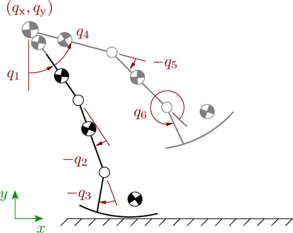
Schematic of the unilateral, transfemoral amputee model during the prosthesis stance period (reproduced from [13]). The prosthetic and human subsystems are shown in black and gray, respectively.

A. Model of the Powered Knee-Ankle Prosthesis

The prosthesis configuration space is given by the set $\mathcal{Q}={\mathrm{ℝ}}^2\times {\mathbb{T}}^3$ with configuration variables q = [q₁, q₂, q₃, q_x, q_y]^T, where (q_x, q_y) is the hip position, q₁ is the absolute thigh angle, q₂ is the knee angle, and q₃ is the ankle angle. The joint velocities of the prosthetic leg are given by the vector $\dot{q}\in {\mathrm{ℝ}}^5$. Therefore, the prosthetic leg state is given by the vector $x={\left[q^T{\dot{q}}^T\right]}^T\in T\mathcal{Q}:=\mathcal{Q}\times {\mathrm{ℝ}}^5$. The dynamics the prosthetic leg are governed by

$$M(q)\ddot{q}+C(q,\dot{q})\dot{q}+G(q)+E{(q)}^T\lambda =Bu+J{(q)}^{T}F,$$ (1)

where M(q) ∈ ℝ^5×5 is the mass matrix, $C(q,\dot{q})\in {\mathrm{ℝ}}^{5\times 5}$ is the matrix of Coriolis/centrifugal forces, G(q) ∈ ℝ⁵ is the vector of gravitational forces, E(q) ∈ ℝ^c×5 is the Jacobian matrix associated with c physical constraints between the foot and the ground, and λ ∈ ℝ^c is the Lagrange multiplier associated with the ground reaction force (GRF). During the prosthetic leg swing phase, E(q) = 0 and λ = 0 because the GRF is zero. We assume no foot slipping during the stance phase. The control torque vector is given by u = [u_k u_a]^T ∈ ℝ², where u_k and u_a are the torque applied to the prosthetic knee and ankle joint, respectively. The matrix B = [0_2×1, I_2×2, 0_2×2]^T ∈ ℝ^5×2 has full rank 2. The socket interaction force vector F = [F_x, F_y, M_z]^T ∈ ℝ³ is exerted at the mid-thigh, which connects the prosthesis to the patient’s body (see Fig. 1). The components F_x, F_y of F are linear forces while the component M_z is a moment in the sagittal plane [12]. The body Jacobian matrix is J(q) = [J₁, 0_3×2] ∈ ℝ^3×5, where

$$J_1=\left[\begin{array}{ccc}1& 0& {\mathcal{l}}_{\text{res}}\cos (q_1)\\ 0& 1& {\mathcal{l}}_{\text{res}}\sin (q_1)\\ 0& 0& 1\end{array}\right]$$ (2)

and ℓ_res is the length of the human’s residual thigh. The body Jacobian maps the force vector F, acting at the beginning of the leg’s kinematic chain, to joint torques/forces. The feet of the human and the prosthetic leg are modeled as arcs with constant curvature as in [13], [21].

B. Model of the Human-Prosthesis Biped

The prosthesis-human, viewed as a single biped, has 8 degrees-of-freedom. We denote the extended configuration vector by $q_e={\left[q^T,q_4,q_5,q_6\right]}^T\in \mathcal{Q}\times {\mathbb{T}}^3$, where q the prosthesis configuration vector, q₄ is the human’s hip (inter-leg) angle, q₅ is the human’s knee angle, and q₆ is the human’s ankle angle.

Following [13], [20], we model bipedal locomotion as a hybrid dynamical system. During the phases of walking, the state is governed by one second-order differential equation during the prosthetic swing phase and another second-order differential equation during the prosthetic stance phase. The transitions between these two phases are governed by two impact maps, which correspond to instantaneous changes in the joint velocities. In particular, the human-prosthesis biped dynamics are given by (see [12], [13], [20], [21] for further details)

$$\begin{array}{rrr}\hfill M_{\mathrm{e}}{\ddot{q}}_{\mathrm{e}}+C_{\mathrm{e}}{\dot{q}}_{\mathrm{e}}+G_{\mathrm{e}}+E_P^T{\lambda }_{\mathrm{P}}=B_{\mathrm{e}}{u}_{\mathrm{e}},& \hfill \text{if}& \hfill p_{\mathrm{H}}(q_{\mathrm{e}})>0\\ \hfill \left(q_{\mathrm{e}}^{+},{{\dot{q}}_{\mathrm{e}}}^{+}\right)={\Delta }_{\mathrm{H}}\left(q_{\mathrm{e}}^{-},{{\dot{q}}_{\mathrm{e}}}^{-}\right),& \hfill \text{if}& \hfill p_{\mathrm{H}}(q_{\mathrm{e}})=0\\ \hfill M_{\mathrm{e}}{\ddot{q}}_{\mathrm{e}}+C_{\mathrm{e}}{\dot{q}}_{\mathrm{e}}+G_{\mathrm{e}}+E_H^T{\lambda }_{\mathrm{H}}=B_{\mathrm{e}}{u}_{\mathrm{e}},& \hfill \text{if}& \hfill p_{\mathrm{P}}(q_{\mathrm{e}})>0\\ \hfill \left(q_{\mathrm{e}}^{+},{{\dot{q}}_{\mathrm{e}}}^{+}\right)={\Delta }_{\mathrm{P}}\left(q_{\mathrm{e}}^{-},{{\dot{q}}_{\mathrm{e}}}^{-}\right),& \hfill \text{if}& \hfill p_{\mathrm{P}}(q_{\mathrm{e}})=0\end{array}$$

where the subscripts P and H are associated with the prosthesis and the human, respectively. Also, the vector $E_i^T{\lambda }_i,i\in \{P,H\}$, is the ground reaction force exerted on the human-prosthesis due to the rolling contact constraint a_i(q) = 0 [13]. The vector u_e = [u^T, u₄, u₅, u₆]^T ∈ ℝ⁵ represents the control torques applied by human and the prosthesis. In particular, the vector u represents the motor torque inputs applied to the prosthesis ankle and knee, while the torques u₄, u₅, u₆ are the human inputs applied at the hip, knee, and ankle joints. The impact mappings relate the human-prosthesis state just before the impact to just after the impact. The impact mappings Δ_H and Δ_P are associated with the human heel-strike and the prosthesis heel-strike, respectively. The function p_i(q_e) ∈ ℝ gives the height of the human/prosthetic swing heel, and the superscripts +/− denote post/pre-impact. Other extended terms are defined as in Section II-A with respect to the coordinate vector q_e.

C. Virtual Constraint Control of Powered Prosthetic Legs

Virtual constraints are relations of the form h(q) = 0 among the joint variables of a legged robot that encode stable walking gaits of the biped [10], [11]. These constraints do not physically exist in the system but are enforced on the robot via feedback control. Motivated by the biological observations in [22], [23], the human behavior is approximated by virtual constraints in [13]. Using a given virtual constraint associated with human walking, an output of the form y = h(q) is designed for the prosthesis, whose stabilization induces stable walking gaits (see [13] for further details). The analysis in [13] demonstrates that the prosthesis-amputee biped would be robust to human-like kinematic variations in the human virtual constraints.

One of the advantages of this control methodology for powered prostheses is that it relieves the designer from dividing a walking gait cycle into numerous phases by considering virtual constraints of the form [13]

$$y=h(q):=h_0(q)-h_d\circ \phi (q)=0,$$ (3)

where h₀(q) := [0_2×1 I_2×2 0_2×2]q, is the vector of the actuated degrees-of-freedom. The function h_d(·), which is a collection of two Bézier polynomials, determines the desired evolution of the actuated joint variables [q₂, q₃]^T as a function of φ(q) [13]. The scalar variable φ(q) is a strictly monotonically increasing variable, which is called the phase variable. Given the virtual constraint in (3), the control objective is to drive y = h(q) and $\dot{y}=(\partial h(q)/\partial q)\dot{q}$ to zero via a PD feedback control law. In the conventional approach [12], [24], [25], the PD control gains are found off-line by trial-and-error. In this paper, we aim to develop a model-free controller that automatically tunes the virtual constraint-based PD gains in real time by using a classical perturbation-based extremum seeking algorithm.

D. Classical Extremum Seeking Algorithm

In order to explain the basic architecture of the standard perturbation-based ESC scheme used in the paper, we consider a system without dynamics, which is given by a static map f(·). The system output y_esc changes instantaneously with the input x. Assuming that f() is a convex function, i.e., f″(x) > 0 for all x, the objective of the ESC scheme is to minimize the output f(x) without knowing a priori the extremum x^∗ of the function f(·).

The ESC scheme block diagram is shown in Fig. 2. In the block diagram, the signal d(t), which is called the dither signal, is a periodic perturbation signal (e.g., sin(ωt)) that is added to the current best estimate of the input x, denoted by $\widehat{x}$. Taking x as input, the mapping f(·) generates the output y_esc = f(x), which is passed through a high pass filter (HPF). The HPF output, denoted by y_H(t), is demodulated by using the same dither signal d(t). The resulting demodulated signal is then passed through a low pass filter (LPF) that generates the output ζ, which is proportional to the gradient of the current measured output y_esc. Next, the signal ζ(t) is passed through an integrator with gain k to give $\widehat{x}$. Since we aim to minimize the objective function, k should be chosen such that the inequality kf″ < 0 holds. This inequality corresponds to moving along the gradient directions along which f(·) decreases. Additional details regarding ESC can be found in [18].

Fig. 2.

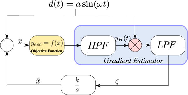
Basic ESC structure (reproduced from [26]).

III. Structure of ESC-based tuning of virtual constraint-based controllers

In this section, we present the structure of our automatic real-time controller tuning method. A rigorous analysis will be presented in the next section.

Given a properly designed virtual constraint h(q) = 0 for a powered prosthetic leg, it should be enforced by driving h(q) and $(\partial h(q)/\partial q)\dot{q}$ towards zero via feedback (see [10] for further details). In this paper, we use the virtual constraints that have been obtained via optimization in [13]. Enforcing the virtual constraints given in [13] results in stable walking of the human-prosthesis biped. In particular, y = h(q) and $\dot{y}=(\partial h(q)/\partial q)\dot{q}$ should be driven to zero using an input-output feedback linearizing control law. Using such a feedback law is not feasible for implementation on the prosthetic leg. This limitation is due to the need for measuring socket interaction forces [13], requiring expensive multi-axis load cells, and the lack of exact knowledge of the prosthetic leg dynamical model parameters. Instead, one can use a PD control law to approximately enforce y and $\dot{y}$ (see [12] for further details). In the conventional virtual constraint-based control algorithms, the PD control gains are tuned in an off-line manner by trial-and-error [12]. These controllers approximately enforce the virtual constraint h(q) = 0, making ║h(q)║ and $\Vert (\partial h(q)/\partial q)\dot{q}\Vert$ sufficiently small to stabilize the walking gait. Hence experimental implementation such as [12], [25] have used a model-free PD control. For these reasons, our paper focuses on auto-tuning of PD control laws for the virtual constraints using a model-free extremum seeking controller.

Our algorithm automatically tunes the virtual constraint-based PD gains in real-time. To achieve this, we consider the following cost function

$$J(q,\dot{q})={\Vert h(q)\Vert }^2+{\Vert \frac{\partial h(q)}{\partial q}\dot{q}\Vert }^2,$$ (4)

and use a control structure, depicted in Fig. 3. Thus, there are two main components: (i) a virtual constraint-based PD controller, given by Γ. The controller Γ commands the prosthetic leg torques via

$$u=-{\theta }_{1}h(q)-{\theta }_2\frac{\partial h(q)}{\partial q}\dot{q},$$ (5)

where

$${\theta }_1=\left[\begin{array}{cc}{\theta }_1^k& 0\\ 0& {\theta }_1^a\end{array}\right],{\theta }_2=\left[\begin{array}{cc}{\theta }_2^k& 0\\ 0& {\theta }_2^a\end{array}\right],$$ (6)

are proportional and damping gain matrices in ℝ^2×2 whose diagonal elements are automatically tuned by the ES scheme. The superscripts k and a correspond to the knee and ankle of the prosthesis, respectively; (ii) a perturbation-based ES scheme whose role is to tune the PD gains given by (6) in real-time, so that the control input u in (5) can minimize the cost function (4).

Fig. 3.

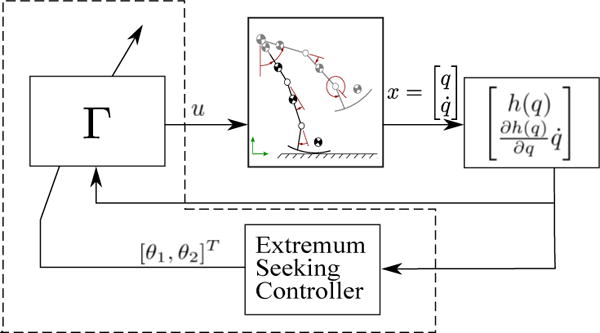
Block diagram of the proposed controller. The controller Γ represents a PD controller, which drives y = h(q) and $(\partial h(q)/\partial q)\dot{q}$ to zero. The PD gains are automatically tuned by four ES loops in real time such that ${\Vert h(q)\Vert }^2+{\Vert (\partial h(q)/\partial q)\dot{q}\Vert }^2$ is minimized.

The cost function J in (4) is the Euclidean distance (squared) of the robot state from the zero dynamics manifold $\mathcal{Z}=\left\{(q,\dot{q}):h(q)=0,\frac{\partial h(q)}{\partial q}\dot{q}=0\right\}$. It can be seen from (4) that J(·) is a function of q, $\dot{q}$. The closed-loop control system trajectories q(t), $\dot{q}(t)$ are the solutions of (1) with control input u, given by (5). Therefore, J(t) is not known in terms of θ₁(t), θ₂(t), a priori. Aside from being C², we do not make any other assumptions on the cost function J. ESC, as a gradient descent algorithm, finds local minima of the cost function J(·) such that the prosthesis closed-loop dynamics are stable.

Assuming that the signal measurements are not noisy, Fig. 4 shows a simplified version of ESC, without filters, used in this paper. Further details regarding the choice of ESC parameters are discussed in Section V.

Fig. 4.

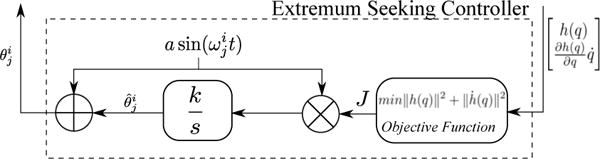
The perturbation-based ES scheme used in the paper.

IV. Closed Loop Dynamics and Stability Analysis

In this section we analyze the stability of the virtual constraint error dynamics along with the ESC dynamics using singular perturbation methods.

Remark 1

In our stability analysis, we only consider the continuous phases of walking, i.e., swing and stance, while ignoring the impacts with the ground. The virtual constraint taken from [13] induces a stable hybrid zero dynamics. Therefore, if the virtual constraint tracking errors become sufficiently small, then the human-prosthesis biped walks in a stable manner (see [12], [24] for further details). ◊

For the sake of brevity, we present our analysis for a symmetric biped. First, we derive the virtual constraint error dynamics for the prosthetic leg. Accordingly, we take two derivatives of y along the vector field of (1). We have

$$\ddot{y}=\frac{d}{dt}\left(\frac{\partial h(q)}{\partial q}\dot{q}\right)=A(q)u+N(q,\dot{q}),$$ (7)

where the matrix $A(q)=\frac{\partial h(q)}{\partial q}{M}^{-1}B\in {\mathrm{ℝ}}^{2\times 2}$ is called the decoupling matrix associated with the virtual constraint y = h(q). The virtual constraints in [13] are designed such that this matrix is non-singular and positive definite. Also,

$$N(q,\dot{q})=\frac{d}{dt}\left(\frac{\partial h(q)}{\partial q}\right)\dot{q}-\frac{\partial h(q)}{\partial q}{M}^{-1}\left\{C(q,\dot{q})\dot{q}+G(q)+E{(q)}^T\lambda -J{(q)}^{T}F\right\},$$ (8)

collects the effect of the nonlinearities in (1).

We denote the PD gain estimates by ${\widehat{\theta }}_j\in {\mathrm{ℝ}}^2$ and use them in (6) to obtain the estimation gain matrices. Next, we substitute the PD control law

$$u=-{\widehat{\theta }}_{1}h(q)-{\widehat{\theta }}_2\frac{\partial h(q)}{\partial q}\dot{q},$$ (9)

into (7) to get

$$\frac{d}{dt}\left(\frac{\partial h(q)}{\partial q}\dot{q}\right)=-A(q)\left({\widehat{\theta }}_{1}h(q)+{\widehat{\theta }}_2\frac{\partial h(q)}{\partial q}\dot{q}\right)+N(q,\dot{q}).$$ (10)

Defining the new state $\stackrel{\sim }{x}:=\left[\begin{array}{c}h(q)\\ \frac{\partial h(q)}{\partial q}\dot{q}\end{array}\right]=\left[\begin{array}{c}{\stackrel{\sim }{x}}_1\\ {\stackrel{\sim }{x}}_2\end{array}\right]\in {\mathrm{ℝ}}^4$, the virtual constraint error dynamics can be written as

$$\dot{\stackrel{\sim }{x}}=\stackrel{\sim }{A}(\stackrel{\sim }{x},\widehat{\theta })\stackrel{\sim }{x}+\stackrel{\sim }{N}(q,\dot{q}),$$ (11)

where

$$\stackrel{\sim }{A}(\stackrel{\sim }{x},\widehat{\theta })=\left[\begin{array}{cc}{0}_{2\times 2}& I_{2\times 2}\\ -A(q){\widehat{\theta }}_1& -A(q){\widehat{\theta }}_2\end{array}\right],\stackrel{\sim }{N}(q,\dot{q})=\left[\begin{array}{c}{0}_{2\times 1}\\ N(q,\dot{q})\end{array}\right].$$ (12)

A single integrator ES loop with dither signal $a\sin ({\omega }_j^{i}t)$ is used for tuning the PD gain ${\theta }_j^i$, where i ∈ {k, a} and j ∈ {1,2} (see Fig. 4). The ES dynamics for the estimate of PD gain ${\theta }_j^i$ can be written as

$${\dot{\widehat{\theta }}}_j^i=\mathit{kaJ}(\stackrel{\sim }{x},{\widehat{\theta }}_j^i)\sin ({\omega }_j^{i}t).$$ (13)

Thus, the augmented closed-loop dynamical equations for the virtual constraint error dynamics are

$$\sum :=\{\begin{array}{l}\dot{\stackrel{\sim }{x}}=\stackrel{\sim }{A}(\stackrel{\sim }{x},\widehat{\theta })\stackrel{\sim }{x}+\stackrel{\sim }{N}(q,\dot{q}),\hfill \\ {\dot{\widehat{\theta }}}_j^i=\mathit{kaJ}(\stackrel{\sim }{x},{\widehat{\theta }}_j^i)\sin ({\omega }_j^{i}t),\text{for}i\in \{k,a\},j\in \{1,2\}\hfill \end{array}$$ (14)

The following result uses a singular perturbation analysis to show that the proposed ESC scheme results in bounded PD gains and small virtual constraint errors.

Proposition 1

Consider the prosthesis virtual constraint error dynamics in (7) along with the ESC-based PD gain update laws in (13). Let ${\widehat{\theta }}_j^{i\ast }$ be the quasi-steady state gain. Then, there exist sufficiently small dither frequencies ${\omega }_j^{i\ast }$ such that for all $0<{\omega }_j^i<{\omega }_j^{i\ast },\left|{\widehat{\theta }}_j^i({\omega }_j^{i}t)-{\widehat{\theta }}_j^{i\ast }({\omega }_j^{i}t)\right|=O({\omega }_j^i)$. Furthermore, ${\widehat{\theta }}_j^{i\ast }({\omega }_j^{i}t)$ satisfies:

$$\begin{gathered} {\widehat{\theta }}_1^{i\ast }({\omega }_j^{i}t)\le {\left({({\widehat{\theta }}_1^i(0))}^3+3\delta Ka{\Vert \mathcal{R}\Vert }^2(1-\cos {\omega }_j^{i}t)\right)}^{1/3} \\ {\widehat{\theta }}_2^{i\ast }({\omega }_j^{i}t)={\widehat{\theta }}_1^{i\ast }({\omega }_j^{i}t)+{\widehat{\theta }}_2^i(0)-{\widehat{\theta }}_1^i(0) \end{gathered}$$ (15)

where $\mathcal{R}=A{(q)}^{-1}N(q,\dot{q})$, Also, $\stackrel{\sim }{x}({\omega }_j^{i}t)-{\stackrel{\sim }{x}}^{\ast }({\omega }_j^{i}t)-z(t)=O({\omega }_j^i)$ where the quasi-steady state tracking error ${\stackrel{\sim }{x}}^{\ast }$ satisfies $\stackrel{\sim }{A}(\stackrel{\sim }{x},\widehat{\theta }){\stackrel{\sim }{x}}^{\ast }+\stackrel{\sim }{N}(q,\dot{q})=0$; and z(t) is the solution. to the boundary layer model $\dot{z}=\stackrel{\sim }{A}(\stackrel{\sim }{x},\widehat{\theta })z$, which is locally asymptotically stable.

Proof

The stability of the error dynamics in (14) is analyzed by a singular perturbation method [27]. To perform the singular perturbation analysis, we bring the closed-loop dynamics in (14) to a standard singular perturbation form. Accordingly, we perform the change of coordinates

$$z=\stackrel{\sim }{x}-{\stackrel{\sim }{x}}^{\ast },$$ (16)

where ${\stackrel{\sim }{x}}^{\ast }$ is the solution¹ to

$$\stackrel{\sim }{A}({\stackrel{\sim }{x}}^{\ast },\widehat{\theta }){\stackrel{\sim }{x}}^{\ast }+\stackrel{\sim }{N}(q,\dot{q})=0.$$ (17)

Expressing the error dynamics given by (14) in terms of the new coordinates in (16), we get

$$\begin{gathered} \dot{z}=\stackrel{\sim }{A}(z+{\stackrel{\sim }{x}}^{\ast },\widehat{\theta })(z+{\stackrel{\sim }{x}}^{\ast })+\stackrel{\sim }{N}(q,\dot{q}) \\ =\stackrel{\sim }{A}(z+{\stackrel{\sim }{x}}^{\ast },\widehat{\theta })z+\stackrel{\sim }{N}(q,\dot{q})+\stackrel{\sim }{A}(z+{\stackrel{\sim }{x}}^{\ast },\widehat{\theta }){\stackrel{\sim }{x}}^{\ast }. \end{gathered}$$ (18)

In the new coordinates (z, $\widehat{\theta }$), the origin (z, $\widehat{\theta }$) = (0, 0) is an equilibrium point because

$$\dot{z}=\stackrel{\sim }{A}({\stackrel{\sim }{x}}^{\ast },0)\underset{=0}{\underbrace{z}}+\underset{=0}{\underbrace{\stackrel{\sim }{N}(q,\dot{q})+\stackrel{\sim }{A}({\stackrel{\sim }{x}}^{\ast },0){\stackrel{\sim }{x}}^{\ast }}}=0.$$ (19)

The overall error dynamics in the new coordinates are

$${\sum }^{\prime }:=\{\begin{array}{l}\dot{z}=\stackrel{\sim }{A}(z+{\stackrel{\sim }{x}}^{\ast },\widehat{\theta })z+\stackrel{\sim }{N}(q,\dot{q})+\stackrel{\sim }{A}(z+{\stackrel{\sim }{x}}^{\ast },\widehat{\theta }){\stackrel{\sim }{x}}^{\ast }\hfill \\ {\dot{\widehat{\theta }}}_j^i=\mathit{kaJ}(z+{\stackrel{\sim }{x}}^{\ast },{\widehat{\theta }}_j^i)\sin ({\omega }_j^{i}t).\hfill \end{array}$$ (20)

Defining $\tau :={\omega }_j^i(t)$ (see Remark 2) and expressing (20) in the new time scale given by τ, we get

$${\sum }^{″}:=\{\begin{array}{l}{\omega }_j^i\frac{dz}{d\tau }=\stackrel{\sim }{A}(z+{\stackrel{\sim }{x}}^{\ast },\widehat{\theta })z+\stackrel{\sim }{N}(q,\dot{q})+\stackrel{\sim }{A}(z+{\stackrel{\sim }{x}}^{\ast },\widehat{\theta }){\stackrel{\sim }{x}}^{\ast }\hfill \\ \frac{d{\widehat{\theta }}_j^i}{d\tau }=\delta \mathit{kaJ}(z+{\stackrel{\sim }{x}}^{\ast },{\widehat{\theta }}_j^i)\sin \tau \hfill \end{array}$$ (21)

where $k:={\omega }_j^i\delta K$ and δ is a small positive constant. According to the singular perturbation theory, we first need to find the quasi-steady state value of z = [z₁ z₂]^T in (21). Accordingly, we set ${\omega }_j^i=0$, corresponding to instantaneous changes of the fast dynamics, and solve the resulting algebraic equations. The algebraic equations, which hold during the quasi-steady state, are given by

$$\stackrel{\sim }{A}(z+{\stackrel{\sim }{x}}^{\ast },\widehat{\theta })z+\stackrel{\sim }{N}(q,\dot{q})+\stackrel{\sim }{A}(z+{\stackrel{\sim }{x}}^{\ast },\widehat{\theta }){\stackrel{\sim }{x}}^{\ast }=0$$ (22)

Substituting $\stackrel{\sim }{A}(z+{\stackrel{\sim }{x}}^{\ast },\widehat{\theta })$and $\stackrel{\sim }{N}(q,\dot{q})$ from (12) in (22), we have

$$\left[\begin{array}{cc}{0}_{2\times 2}& I_{2\times 2}\\ -A(q){\widehat{\theta }}_1& -A(q){\widehat{\theta }}_2\end{array}\right]\left[\begin{array}{c}{z}_1\\ z_2\end{array}\right]+\left[\begin{array}{c}{0}_{2\times 1}\\ N(q,\dot{q})\end{array}\right]+\left[\begin{array}{cc}{0}_{2\times 2}& I_{2\times 2}\\ -A(q){\widehat{\theta }}_1& -A(q){\widehat{\theta }}_2\end{array}\right]\left[\begin{array}{c}{\stackrel{\sim }{x}}_1^{\ast }\\ {\stackrel{\sim }{x}}_2^{\ast }\end{array}\right]=\left[\begin{array}{c}{0}_{2\times 1}\\ 0_{2\times 1}\end{array}\right].$$ (23)

Solving for z, we get

$$z_2=-{\stackrel{\sim }{x}}_2^{\ast };z_1={\widehat{\theta }}_1^{-1}\mathcal{R}-{\stackrel{\sim }{x}}_1^{\ast },$$ (24)

where $\mathcal{R}=A{(q)}^{-1}N(q,\dot{q})$. Having found the quasi-steady state values of z₁ and z₂, the objective function J(·) in (21), denoted by J_qs, evaluated at the quasi-steady state is

$$J_{qs}({\widehat{\theta }}_1,{\widehat{\theta }}_2)={\Vert z_1+{\stackrel{\sim }{x}}_1^{\ast }\Vert }^2+{\Vert z_2+{\stackrel{\sim }{x}}_2^{\ast }\Vert }^2={\Vert {\widehat{\theta }}_1^{-1}\mathcal{R}\Vert }^2,$$ (25)

where $\mathcal{R}$ is a constant vector in the slow time-scale $\tau ={\omega }_j^{i}t$. Note that J_qs is only a function of ${\widehat{\theta }}_1$. It remains to show that the ESC dynamics for ${\widehat{\theta }}_1$ at the quasi-steady state is stable. The ESC dynamics (21) can then be written as

$$\frac{d{\widehat{\theta }}_j^{i\ast }}{d\tau }=\delta Ka{J}_{qs}({\widehat{\theta }}_1)\sin \tau ,$$ (26)

where ${\widehat{\theta }}_j^{i\ast }$ is the gain evaluated at the quasi-steady state. Equation (26) represents a reduced system. Plugging the value of J_qs in (26), we get

$$\frac{d{\widehat{\theta }}_j^{i\ast }}{d\tau }=\delta Ka{\Vert {\widehat{\theta }}_1^{-1}\mathcal{R}\Vert }^2\sin \tau .$$ (27)

Using submultiplicative property of 2-norm, we get

$$\begin{gathered} \frac{d{\widehat{\theta }}_j^{i\ast }}{d\tau }\le \delta Ka{\Vert {\widehat{\theta }}_1^{-1}\Vert }^2{\Vert \mathcal{R}\Vert }^2\sin \tau \\ =\frac{\delta Ka{\Vert \mathcal{R}\Vert }^2}{{\lambda }_{\mathit{max}}\left({\widehat{\theta }}_1^T{\widehat{\theta }}_1\right)}\sin \tau =\frac{\delta Ka{\Vert \mathcal{R}\Vert }^2}{{\lambda }_{\mathit{max}}\left({\widehat{\theta }}_1^{k^2},{\widehat{\theta }}_1^{a^2}\right)}\sin \tau . \end{gathered}$$ (28)

Analyzing (28) for i = a, we have

$$\frac{d{\widehat{\theta }}_j^{a\ast }}{d\tau }\le \frac{\delta Ka{\Vert \mathcal{R}\Vert }^2}{{\left({\widehat{\theta }}_1^{a\ast }(\tau )\right)}^2}\sin \tau .$$ (29)

Setting j = 1 and integrating both sides of (29) from τ = 0 to $\tau ={\omega }_j^{i}t$, we get,

$${\widehat{\theta }}_1^{a\ast }({\omega }_j^{i}t)\le {\left({({\widehat{\theta }}_1^a(0))}^3+3\delta Ka{\Vert \mathcal{R}\Vert }^2(1-\cos ({\omega }_j^{i}t))\right)}^{1/3}$$ (30)

Similar argument holds for i = k. From (27), it is clear that

$$\frac{d{\widehat{\theta }}_1^{i\ast }}{d\tau }=\frac{d{\widehat{\theta }}_2^{i\ast }}{d\tau }$$ (31)

since the right hand side of (27) is a only a function of ${\widehat{\theta }}_1$. Integrating both sides of (31) from τ = 0 to $\tau ={\omega }_j^{i}t$, we get,

$${\widehat{\theta }}_2^{i\ast }({\omega }_j^{i}t)={\widehat{\theta }}_1^{i\ast }({\omega }_j^{i}t)+{\widehat{\theta }}_2^i(0)-{\widehat{\theta }}_1^i(0)$$ (32)

Thus, equation (30), (32) shows that the stiffness and damping gains always remain bounded, as claimed in (15).

Now we perform a boundary layer model analysis. Taking the time derivative of (16), we get

$$\begin{gathered} \dot{z}=\dot{\stackrel{\sim }{x}}-{\dot{\stackrel{\sim }{x}}}^{\ast }=\stackrel{\sim }{A}(\stackrel{\sim }{x},\widehat{\theta })\stackrel{\sim }{x}+\stackrel{\sim }{N}(q,\dot{q}), \\ =\stackrel{\sim }{A}(\stackrel{\sim }{x},\widehat{\theta })\stackrel{\sim }{x}-\stackrel{\sim }{A}({\stackrel{\sim }{x}}^{\ast },\widehat{\theta }){\stackrel{\sim }{x}}^{\ast }, \end{gathered}$$ (33)

where $\stackrel{\sim }{N}(q,\dot{q})=-\stackrel{\sim }{A}({\stackrel{\sim }{x}}^{\ast },\widehat{\theta }){\stackrel{\sim }{x}}^{\ast }$ from (17). Equation (33) can be written in terms of z as

$$\dot{z}=\stackrel{\sim }{A}(z+{\stackrel{\sim }{x}}^{\ast },\widehat{\theta })z+\left[\stackrel{\sim }{A}(z+{\stackrel{\sim }{x}}^{\ast },\widehat{\theta })-\stackrel{\sim }{A}({\stackrel{\sim }{x}}^{\ast },\widehat{\theta })\right]{\stackrel{\sim }{x}}^{\ast }.$$ (34)

The first order Taylor series expansion of the right hand side of (34) about z = 0 is

$$\dot{z}=\left({\frac{d}{dz}\stackrel{\sim }{A}(z+{\stackrel{\sim }{x}}^{\ast },\widehat{\theta })z|}_{z=0}\right)z+\left[{\stackrel{\sim }{A}({\stackrel{\sim }{x}}^{\ast },\widehat{\theta })+\frac{d}{dz}\stackrel{\sim }{A}(z+{\stackrel{\sim }{x}}^{\ast },\widehat{\theta })z|}_{z=0}-\stackrel{\sim }{A}({\stackrel{\sim }{x}}^{\ast },\widehat{\theta })\right]{\stackrel{\sim }{x}}^{\ast },$$ (35)

which can be shown to be

$$\dot{z}=\left({\frac{d}{dz}\stackrel{\sim }{A}(z+{\stackrel{\sim }{x}}^{\ast },\widehat{\theta })z|}_{z=0}\right)z=\stackrel{\sim }{A}({\stackrel{\sim }{x}}^{\ast },\widehat{\theta })z.$$ (36)

Since A(q) is positive definite, $\stackrel{\sim }{A}({\stackrel{\sim }{x}}^{\ast },\widehat{\theta })$ is negative definite, proving the boundary layer model to be locally asymptotically stable. Using Theorem 11.1 in [27] concludes the proof.

Remark 2

In the standard ES perturbation-based schemes, the ES loop dynamics need to be run much slower than the plant dynamics. This is achieved by choosing a small dither frequency such that a time scale separation holds between the ES loop and the plant dynamics.

V. Simulation Results

A complete biped system comprising the human and the prosthesis subsystem was simulated as in [13]. The human subsystem was controlled using input-output feedback linearization with fixed PD gains to enforce the virtual constraints defined in [13], which predict certain features of human walking. The prosthesis subsystem was controlled by the model-free output PD controller (5), which assumes no knowledge of the human system. The total leg length of the model was 90.1 cm, and the mass of the prosthetic leg was 5.7 kg. The Cartesian coordinate of the hip position, i.e., q_x, was chosen as a phase variable. The ESC method from Section III was used to continuously modify the PD gains. To demonstrate the effectiveness of ESC in adapting the gains, simulations were carried out on two different models with its total mass equal to 69.1 and 103.1 kg. The dither amplitude was selected as a = 2 with dither frequencies ${\omega }_1^k=1.4$, ${\omega }_1^a=1.8$, ${\omega }_2^k=1.6$, and ${\omega }_2^a=1.2\text{rad/s}$, and the integrator gains were selected as k = 350. The initial values of PD gains were selected as ${\theta }_1^k={\theta }_1^a=10$ and ${\theta }_2^k={\theta }_2^a=1$. The frequency of the dither was chosen small for two reasons: (i) Theoretically, this allows sufficient time-scale separation between the ESC dynamics [18] and the plant dynamics (human and prosthesis), which have frequencies from 16π to 32π rad/s during walking [28]; (ii) Practically, choosing the dither frequency much smaller than the joint motion frequencies induced by virtual constraints does not result in erratic changes in the control input.

The stabilizing effect of the PD controller, coupled with ESC adaptation, is acutely illustrated in Fig. 5. The amputee biped using fixed PD gains falls after a few steps. However, the amputee biped controlled with a PD controller coupled with ESC adaptation is able to walk stably over 60 steps with the initial gains much lower than the fixed PD controller. Fig. 6 shows the adaptation of PD gains for amputees of different weights. A supplemental simulation video can be found at https://youtu.be/c-D_h63NnZw. As opposed to [7], which does not tune the damping gains, our method helps find the optimum values for different amputees.

Fig. 5.

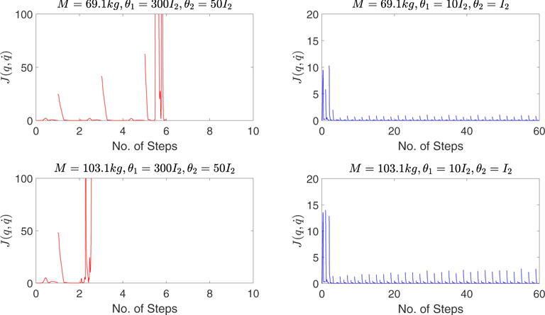
Plots of the objective function for models with two different masses. Left: fixed PD gains. Right: proposed ESC-tuned gains.

Fig. 6.

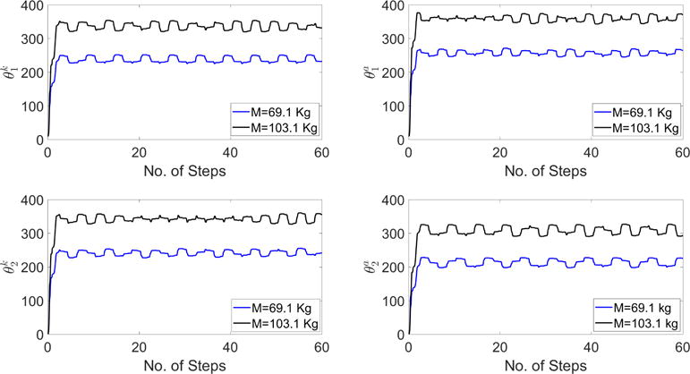
Optimization of stiffness and damping gains of a impedance controller for amputees of different weights.

VI. Conclusion

In this paper, we presented an automatic tuning scheme for virtual constraint-based control laws for a powered knee and ankle prosthesis. The proposed algorithm, which is based on a standard perturbation-based ESC, runs in real-time and does not require knowing the parameters of the human-prosthesis biped. Simulation studies demonstrate the effectiveness of our control methodology. In our future work, a real-time, model-free multi-objective optimization will be used to consider multiple conflicting objectives, e.g., tracking error vs. energy consumed. We will also test our approach on a real powered prosthetic leg against a wider range of uncertain amputee physiological parameters.

References

- 1.Hogan N. Impedance control: An approach to manipulation: Part II -Implementation. J Dyn Syst Meas Contr. 1985;107(1):8–16. [Google Scholar]
- 2.Tucker MR, Olivier J, Pagel A, Bleuler H, Bouri M, Lambercy O, del R Millán J, Riener R, Vallery H, Gassert R. Control strategies for active lower extremity prosthetics and orthotics: a review. J Neuroeng Rehabil. 2015;12(1) doi: 10.1186/1743-0003-12-1. [DOI] [PMC free article] [PubMed] [Google Scholar]
- 3.Sup F, Varol HA, Goldfarb M. Upslope walking with a powered knee and ankle prosthesis: initial results with an amputee subject. IEEE Trans Neur Syst Rehab Eng. 2011;19(1):71–78. doi: 10.1109/TNSRE.2010.2087360. [DOI] [PubMed] [Google Scholar]
- 4.Shultz A, Lawson B, Goldfarb M. Running with a powered knee and ankle prosthesis. IEEE Trans Sys Rehab Eng. 2015;23(3):403–412. doi: 10.1109/TNSRE.2014.2336597. [DOI] [PubMed] [Google Scholar]
- 5.Lawson B, Varol H, Huff A, Erdemir E, Goldfarb M. Control of stair ascent and descent with a powered transfemoral prosthesis. IEEE Trans Neur Sys Rehab Eng. 2013;21(3):466–473. doi: 10.1109/TNSRE.2012.2225640. [DOI] [PubMed] [Google Scholar]
- 6.Simon AM, Ingraham KA, Fey NP, Finucane SB, Lipschutz RD, Young AJ, Hargrove LJ. Configuring a powered knee and ankle prosthesis for transfemoral amputees within five specific ambulation modes. PloS one. 2014;9(6):e99387. doi: 10.1371/journal.pone.0099387. [DOI] [PMC free article] [PubMed] [Google Scholar]
- 7.Wang D, Liu M, Zhang F, Huang H. Design of an expert system to automatically calibrate impedance control for powered knee prostheses. IEEE Int Conf Rehabil Robot. 2013:1–5. doi: 10.1109/ICORR.2013.6650442. [DOI] [PubMed] [Google Scholar]
- 8.Aghasadeghi N, Zhao H, Hargrove LJ, Ames AD, Perreault EJ, Bretl T. Learning impedance controller parameters for lower-limb prostheses. 2013 IEEE/RSJ International Conference on Intelligent Robots and Systems IEEE. 2013:4268–4274. [Google Scholar]
- 9.Huang H, Crouch DL, Liu M, Sawicki GS, Wang D. A cyber expert system for auto-tuning powered prosthesis impedance control parameters. Annals of Biomedical Engineering. 2016;44(5):1613–1624. doi: 10.1007/s10439-015-1464-7. [DOI] [PubMed] [Google Scholar]
- 10.Westervelt E, Grizzle J, Chevallereau C, Choi J, Morris B. Feedback Control of Dynamic Bipedal Robot Locomotion. New York, NY: CRC Press; 2007. [Google Scholar]
- 11.Sreenath K, Park HW, Poulakakis I, Grizzle JW. A compliant hybrid zero dynamics controller for stable, efficient and fast bipedal walking on MABEL. Int J Robot Res. 2011;30(9):1170–1193. [Google Scholar]
- 12.Gregg RD, Lenzi T, Hargrove LJ, Sensinger JW. Virtual constraint control of a powered prosthetic leg: From simulation to experiments with transfemoral amputees. IEEE Trans Robotics. 2014;30(6):1455–1471. doi: 10.1109/TRO.2014.2361937. [DOI] [PMC free article] [PubMed] [Google Scholar]
- 13.Martin AE, Gregg RD. Stable, robust hybrid zero dynamics control of powered lower-limb prostheses. IEEE Trans Automat Contr. 2017 doi: 10.1109/TAC.2017.2648040. [DOI] [PMC free article] [PubMed] [Google Scholar]
- 14.Mohammadi A, Rezapour E, Maggiore M, Pettersen KY. Maneuvering control of planar snake robots using virtual holonomic constraints. IEEE Trans Contr Syst Technol. 2016;24(3):884–899. [Google Scholar]
- 15.Kohl AM, Kelasidi E, Mohammadi A, Maggiore M, Pettersen KY. Planar maneuvering control of underwater snake robots using virtual holonomic constraints. Bioinspiration & Biomimetics. 2016;11(6):065005. doi: 10.1088/1748-3190/11/6/065005. [DOI] [PubMed] [Google Scholar]
- 16.Rezapour E, Hofmann A, Pettersen KY, Mohammadi A, Maggiore M. Virtual holonomic constraint based direction following control of planar snake robots described by a simplified model. IEEE Conf Contr Applicat. 2014:1064–1071. [Google Scholar]
- 17.Nguyen Q, Sreenath K. L1 adaptive control for bipedal robots with control lyapunov function based quadratic programs. American Contr Conf. 2015:862–867. [Google Scholar]
- 18.Krstić M, Wang H-H. Stability of extremum seeking feedback for general nonlinear dynamic systems. Automatica. 2000;36(4):595–601. [Google Scholar]
- 19.Ariyur KB, Krstic M. Real-time optimization by extremum-seeking control. John Wiley & Sons; 2003. [Google Scholar]
- 20.Gregg RD, Martin AE. Prosthetic leg control in the nullspace of human interaction. American Contr Conf. 2016:4814–4821. doi: 10.1109/ACC.2016.7526115. [DOI] [PMC free article] [PubMed] [Google Scholar]
- 21.Martin A, Post D, Schmiedeler J. Design and experimental implementation of a hybrid zero dynamics controller for planar bipeds with curved feet. Int J Robot Res. 2014;33(7):988–1005. [Google Scholar]
- 22.Gregg RD, Rouse EJ, Hargrove LJ, Sensinger JW. Evidence for a time-invariant phase variable in human ankle control. PloS one. 2014;9(2):e89163. doi: 10.1371/journal.pone.0089163. [DOI] [PMC free article] [PubMed] [Google Scholar]
- 23.Villarreal DJ, Poonawala HA, Gregg RD. A robust parameterization of human gait patterns across phase-shifting perturbations. IEEE Trans Neur Sys Rehab Eng. 2017;25(3):265–278. doi: 10.1109/TNSRE.2016.2569019. [DOI] [PMC free article] [PubMed] [Google Scholar]
- 24.Quintero D, Martin AE, Gregg RD. Toward unified control of a powered prosthetic leg: A simulation study. IEEE Trans Contr Syst Technol. 2017;PP(99):1–8. doi: 10.1109/TCST.2016.2643566. [DOI] [PMC free article] [PubMed] [Google Scholar]
- 25.Quintero D, Villarreal DJ, Gregg RD. Preliminary experiments with a unified controller for a powered knee-ankle prosthetic leg across walking speeds. IEEE/RSJ Int Conf Intell Robot Syst. 2016:5427–5433. doi: 10.1109/IROS.2016.7759798. [DOI] [PMC free article] [PubMed] [Google Scholar]
- 26.Kumar S, Gans N. Extremum seeking control for multi-objective optimization problems. IEEE Conf Dec Contr. 2016:1112–1118. [Google Scholar]
- 27.Khalil HK. Noninear Systems. Prentice-Hall; New Jersey: 1996. [Google Scholar]
- 28.Winter DA. Biomechanics and motor control of human movement. John Wiley & Sons; 2009. [Google Scholar]