Survival models and health sequences

Abstract

Survival studies often generate not only a survival time for each patient but also a sequence of health measurements at annual or semi-annual check-ups while the patient remains alive. Such a sequence of random length accompanied by a survival time is called a survival process. Robust health is ordinarily associated with longer survival, so the two parts of a survival process cannot be assumed independent. This paper is concerned with a general technique—reverse alignment—for constructing statistical models for survival processes, here termed revival models. A revival model is a regression model in the sense that it incorporates covariate and treatment effects into both the distribution of survival times and the joint distribution of health outcomes. The revival model also determines a conditional survival distribution given the observed history, which describes how the subsequent survival distribution is determined by the observed progression of health outcomes.

1 Survival studies

A survival study is one in which patients are recruited according to well-defined selection criteria and their health status monitored on a regular or intermittent schedule until the terminal event. Covariates such as sex and age are recorded at the time of recruitment, and, if there is more than one treatment level, the assignment is presumed to be randomized. In a simple survival study, the health status Y(t) at time t is a binary variable, dead or alive, and the entire process is then summarized by the time T > 0 spent in state 1, i.e., the survival time. In a survival study with health monitoring, Y(t) is a more detailed description of the state of health or quality of life of the individual, containing whatever information—pulse rate, cholesterol level, cognitive score or CD4 cell count—is deemed relevant to the study. The goal may be to study the effect of treatment on survival time, or to study its effect on quality of life, or to predict the subsequent survival time of patients given their current health history.

Survival studies with intermittent health monitoring are moderately common, and likely to become more so as health records become available electronically for research purposes. Within the past few years, several issues of the journal Lifetime Data Analysis have been devoted to problems connected with studies of exactly this type. For a good introduction, with examples and a discussion of scientific objectives, see Diggle, Sousa and Chetwynd (2006), Kurland, Johnson, Egleston and Diehr (2009) or Farewell and Henderson (2010). Section 8 of van Houwelingen and Putter (2012) is recommended reading.

In practice, the patient's health status is measured at recruitment (t = 0), and regularly or intermittently thereafter while the patient remains alive. To emphasize the distinction between the observation times and observation values, each time is called an appointment date; the set of dates is called the appointment schedule. Apart from covariate and treatment values, a complete uncensored observation on one patient (T, t, Y[t]) consists of the survival time T > 0, the appointment schedule t ⊂ [0, T), and the health status measurements Y[t] at these times. To accommodate patients whose record is incomplete, a censoring indicator variable (Δ) is also included. In that case, the censoring time is usually, but not necessarily, equal to the date of the most recent appointment.

A statistical model for a survival study is a family of probability distributions for the record of each patient, all three components included. At a minimum, therefore, it is necessary to model the survival time and the state of health jointly, and to consider how the joint distribution might be affected by treatment. Ordinarily, robust health is associated with longevity, but if both are affected by treatment, there is no guarantee that the two effects are in similar directions.

In the sense that the health status is measured over time on each patient, a survival study is a particular sort of longitudinal study. Certainly, temporal and other correlations are expected and must be accommodated. But the distinguishing feature, that each sequence is terminated by failure or censoring, gives survival-process models a very distinct character: death, as an absorbing state, contradicts stationarity in an extreme way. For a good survey of the goals of such studies and the modeling strategies employed, see Kurland, Johnson, Egleston and Diehr (2009).

The goal of this paper is to explore a general mathematical framework for the construction of survival-process models built upon this distinguishing feature by considering reverse alignment of the health processes. The framework permits easy computation of the likelihood function and parameter estimates, and straightforward derivation of predictive distributions for individual survival times. The chief motivation for these models is the effective alignment of patient records for pattern matching and signal extraction. Our framework permits asking whether alignment by patient age, by recruitment date, or by time remaining to failure is most effective. Of course, a hybrid of alignments may be most effective and our framework allows for this possibility. Apart from reservations concerning the use of time-evolving covariates, all standard survival models are acceptable within the framework. Administrative complications of the sort that are inevitable in medical and epidemiological research will be ignored for the most part. Discussion of computational techniques needed for model fitting and parameter estimation is provided in Section 5.2; however, the emphasis is on statistical ideas and principles, strategies for model formulation, sampling schemes, and the distinction between time-dependent variables and time-evolving variables in the definition of treatment effects.

2 Related work

The medical and biostatistical literature contains numerous examples of studies involving both successive measurements on each patient, such as CD4 lymphocyte cell counts, together with survival time (Lagakos, 1976; DeGruttola and Tu, 1994; Faucett and Thomas 1996; Guo and Carlin, 2004; Fieuws, Ver-beke, Maes and Vanrenterghem, 2008). Geriatric studies seldom focus exclusively on survival time, but tend to emphasize variables related to quality of life, such as overall physical and mental health, mobility, independence, memory loss, mental acuity, and so on. In the statistical literature, survival studies with health monitoring are called longitudinal studies with time-to-event data (Wulfsohn and Tsiatis, 1997; Henderson, Diggle and Dobson, 2000; Xu and Zeger, 2001; Tsiatis and Davidian, 2004; Rizopoulos, 2012). Although there are variations in model formulation and implementation, all authors are agreed on the need for a joint distribution covering both survival time and the progression of health outcomes; see Hsieh et al. (2006), Ding and Wang (2008), and Albert and Shih (2010) for additional references.

There are two widely used approaches for longitudinal data analysis with non-ignorable terminal event: a latent-variable approach and a marginal estimating equation approach using inverse probability weighting. The estimating equation approach is inappropriate when the event is terminal as the method treats the terminal event as only a censoring of the longitudinal measurements. Below we describe the latent-variable approach in some detail. This jointly models the survival time and health process via a latent temporal process. We present the well-known shared parameter model (Tsiatis and Davidian, 2004; Rizopoulos, 2012) as a particular example of this approach.

A common joint modeling approach begins with a pair (η, T) consisting of a latent temporal process η(t) together with a positive random variable T < ∞. This joint distribution determines the distribution of the observable process¹

$$Y(t)=\{\begin{array}{cc}\eta (t)& t<T\\ ♭& t\ge T\end{array}$$ (1)

by restriction of the latent process to (−∞, T), or by censoring at time T. The observable process Y constructed in this way has the same domain t ∈ R as the unobservable process η, but the state space includes an additional absorbing value, here labelled ♭. Equivalently, but slightly less conveniently, Y may be defined as a process on the random domain (−∞, T) or (0, T). In either case the survival time T is a function of Y.

In the simplest case where the latent process is Gaussian, η ∼ GP(μ, K) on R, the distributions for each finite subset t ⊂ R are Gaussian:

$$\eta [\mathbf{t}]~N(\mu [\mathbf{t}],K[\mathbf{t}]).$$

This is not to be confused with the distribution of the observable process (t, Y[t]) at either a fixed or randomly generated set of appointment dates. For fixed t, the implied restriction to survivors {i: T_i > max(t)} is an instance of truncation or preferential sampling (McCullagh, 2008; Diggle, Menezes and Su, 2010), and the distribution among survivors is not Gaussian.

A more explicit example is given by Rizopoulos (2012). Given the real-valued temporal process m(t), the survival distribution is determined by the conditional hazard function

$$h(t)=h_0(t)exp\{{\gamma }^{T}w+\alpha m(t)\}$$ (2)

where w is a vector of baseline covariates, and h₀(·) is a baseline risk function common among all patients. The survival time and the latent health process η(t) = m(t) + ∊(t) are conditionally independent given {m(t)}_t≥0, and the observable health process Y is given by equation (1). In the literature on joint modeling, m(t) is called the “true and unobserved” state of health, which is not limited to t < T. For a more detailed account of specific processes, see Rizopoulos (2012), or chapters 13–16 of Fitzmaurice, Davidian, Verbeke and Molenberghs (2009).

The latent-variable framework contains the shared parameter model (Ten Have et al., 2000; Tsiatis and Davidian, 2004). In this model, the state of health for patient i, m_i(t), is described by a linear mixed effects models

$$m_i(t)=x_i{(t)}^T\beta +z_i{(t)}^T{b}_i$$

where β is a vector of fixed effects with corresponding covariate vector x_i(t), b_i is a vector of (typically Gaussian) random effects with corresponding covariate vector z_i(t). The b_i are shared frailties (i.e., subject-specific characteristics). Setting z_i(t)^Tb_i = b_0i + b_1it, for example, incorporates both a random intercept to characterize a baseline level and random slope to characterize a subject-specific trend in the true health trajectory. The shared parameter model uses these latent frailties to indirectly model the relationship between the the health process and the survival distribution. The particular model above is an example of the standard shared parameter model. Of course, it can be extended in several natural ways. For example, we may consider a complex functional representation such as a spline regression. There is continued research around this formulation. For two recent examples, Li et al. (2009) consider a semiparametric approach to estimation, while Crowther et al. (2016) incorporate delayed entry and assessment of model misspecification. In certain circumstances the health process is a point process, recording the occurrences of a specific type of non-fatal event. The shared parameter model has been extended to this setting (Huang and Wang (2004), Zeng and Lin (2009)). In Section 4.4, we illustrate joint modeling of recurrent events and a terminal event under reverse-alignment.

The latent-variable model (and by inclusion the shared parameter model) seems natural enough for recurrent non-fatal events, but probability distributions constructed in this way are extraordinarily complicated when applied to single-event survival data. In particular, the model defines health-status trajectories beyond death. What is missing is an explicit recognition of the fact that death is a state of health, arguably the defining characteristic of a health process, and certainly not a censoring event. Often m(t) is referred to as the “immortal process” as it is well-defined for all t > 0, which may be applicable when the event is dropout. However, death is the fundamental characteristic of a survival process.

2.1 Prior work on reverse alignment

In order to avoid some of the technical difficulties associated with joint modeling the suggestion put forward in this paper is to approach the problem from a different angle—literally in reverse. Reverse alignment avoids the intermediate recurrent process by considering probability distributions for the non-recurrent observable process Y directly. It is discussed as one of several options in Table 2 of Kurland, Johnson, Egleston and Diehr (2009), and is mentioned in section 8.3 of van Houwelingen and Putter (2012), so the idea is not new.

Table 2. ANOVA decomposition for Table 1.

Source	𝒰/𝒱	‖P𝒰Y‖2 – ‖P𝒱Y‖2	d.f.	M.S.
Diagonal	(R + C +D)/(R + C)	544.3	7	77.8
Column	(R + C + D)/(R + D)	237.9	7	34.0
Row	(R + C + D)/(C + D)	817.3	7	116.8
Residual	RC/(R+ C + D)	497.2	21	23.7

Estimation of reverse time-models has been considered by several authors. Chan and Wang (2010) consider a nonparametric estimation approach for the mean of the reverse-time process. They investigate end-of-life-cost for ovarian cancer cases diagnosed at age 65 or older among Medicare enrolles. Li et al. (2013) consider a likelihood-based approach for the reverse-time model with applications to palliative care. The approach extends the terminal decline model introduced by Kurland et al. (2009) to include a survival model that incorporates subjects with censored records. Li et al. (2017) considers a semiparametric approach to the same terminal decline model. Finally, shortly before final acceptance of this paper, a referee informed us about the forthcoming paper by Kong et al. (2017), which to some extent touches on similar topics as this work. Kong et al. propose a two-stage semiparametric likelihood based approach. The paper presents a hybrid approach that incorporates features of time since recruitment along with terms that capture nonlinear terminal behavior that enter only as the participant approaches the terminal event.

This paper explores the probabilistic and statistical implications of time-reversal. It builds from the novel conceptual insight that the health process and survival distribution are not simply correlated, but are in fact a single health process when the event is terminal. Health processes are characterized by the notion of flatlining and the survival time is a deterministic function of the health process. In section 3.4, we present a simple analysis of variance technique to investigate whether reverse-time modeling is more appropriate for a particular dataset than forward-time modeling.

We then present a novel investigation into several statistical consequences of reverse-time modeling: implications for sampling, consequences for survival prediction, and the interpretation and estimation of treatment effects. In prior work, the appointment schedule is pre-determined (e.g., Kong pp. 4, (2017)) and fixed. Here we consider a variety of appointment schedules. We present the sequential conditional independence condition under which we can perform simple likelihood estimation using uncensored records. We fit simple Poisson point process models to show how this condition leads to very weak assumptions on the appointment schedule. In Section 4, we illustrate prediction and how the conditional density depends on both the distribution of the appointment schedule and the revival model. Namely, we introduce the notion of stale measurements. We show predictive distributions based on reverse-time models often exhibit weak dependence on measurements made sufficiently far in the past. In Section 3.5, we define the treatment protocol and the necessary assumption of lack of interference. We then follow this with a discussion of the interpretation of treatment effects in Section 5.3. When aligning by failure, we recognize the importance of introducing a null level for treatment at times before and including baseline.

While prior work has incorporated the proportional-hazards specification for the survival distribution, we discuss complications that arise under the Cox proportional-hazards model. Namely, alignment by failure requires the survival time to be finite with probability one. We present several ways to address this issue. We build upon prior work on Markov, exchangeable survival processes to construct survival models similar to the Cox proportional-hazards model but which guarantee the survival times are finite with probability one. Covariates and treatment can be readily incorporated.

Finally, as in Kong et. al (2017) we provide a systematic approach to considering behavior related to time since recruitment. Our modeling approach captures terminal behavior via nonlinear functions of time until failure. For example, we consider the logarithm of reverse-time in the model introduced in Section 6. We also introduce nonlinear dependence on time until failure into the distribution of the appointment schedule in section 4.5 via an inverse linear model. In both instances, the behavior away from the terminal event depends weakly on these terms. We also incorporate features related to time since recruitment. We provide a simple likelihood-ratio test to ensure we have captured all important forward behavior. See Section 5.1.2 for further details.

3 Reverse alignment

3.1 The survival process

A survival process Y is a stochastic process defined for real t, in which Y_i(t) is the state of health or quality of life of patient i at time t, usually measured from recruitment. In a simple survival process, the state space ℛ = {0, 1} is sufficient to encode only the most basic of vital signs, dead or alive; more generally, the state space is any set large enough to encode the observable state of health or quality of life of the patient at one instant in time. Flatlining, introduced in equation (1), is the distinguishing characteristic of a survival process, i.e., ♭ ∈ ℛ is an absorbing state such that Y(t) = ♭ implies Y(t′) = ♭ for all t′ ≥ t. The survival time is a deterministic function of the survival process:

$$T_i=\underset{t\ge 0}{sup}\{t:Y_i(t)\ne ♭\};$$

it is presumed that Y_i(0) ≠ ♭ at recruitment, so T_i > 0. This definition is quite general, and does not exclude immortality, i.e., T = ∞ with positive probability. Multiple absorbing states {♭_c} representing different terminal events may occur. In all of the models considered here, however, survival time is finite with probability one. Anonymous (2016) provide an indepth discussion of the concepts of vital variables and independent evolution, key ideas for stochastic processes associated with the survival process.

A key distinction from prior work is our understanding of the health process as a single stochastic process. This is opposed to the standard approach of considering two correlated stochastic processes. The latter interpretation is defensible when the event is not terminal; however, for terminal events this is simply not the case. Note, the state ♭ ∈ ℛ is arbitrary and only important in so far as it denotes the health process has flatlined. Consider, for example, a health process where Y_i(t) for t < T is some biomarker index taking values in R. Then ℛ = R ⋃ ♭. Of course, if the index takes values in the positive reals R₊, the state ♭ can be set to an arbitrary negative real. The important thing is that ♭ be distinguished from the rest of the state-space.

3.2 Statistical modeling strategies

At least three distinct strategies may be identified for constructing a survival process, meaning an explicit or implicit probabilistic specification of a continuous-time stochastic process having one or more absorbing states.

One classical approach is to specify the process by its instantaneous transition intensity, or infinitesimal generator q(y′ ↦ dy; dt) in the case of a Markov process. This ‘stochastic differential-equation’ approach generates a random health trajectory in continuous time in much the same way that a partial differential equation generates a non-random trajectory for the motion of particles in a fluid. In principle, the finite-dimensional distribution P_τ(y) is obtained by integration over all paths that are equal to y = (y₁, …, y_k) at the specified set of times τ = (τ₁, …, τ_k). Explicit integration is feasible for stationary Markov processes, but non-stationary non-Markov processes present formidable technical difficulties.

A statistical model requires a family of transition intensities, which means that the effect of treatment and covariates on the transition intensity must be specified. For a pure survival process with state space {0, 1} and no marker variables, the instantaneous transition intensity 1 ↦ 0 is called the hazard function; the multiplicative factor in the proportional-hazards model specifies the effect of treatment and/or covariates on the hazard and thence on the distribution of survival times. For this special setting, there is no need to integrate over paths because 0 = ♭ is the absorbing state, and Y(t) is observable in continuous time.

For the simplest Markovian setting with non-binary state space, the transition intensity for a control patient is q₀(y′ ↦ dy; dt) for y′ ∈ R and y ∈ ℛ. In what way should be the transition intensity be modified by treatment? It seems natural to split q₀ into a sub-stochastic diffusion R → R while the patient lives, plus an absorption intensity y′ ↦ ♭, and to specify treatment effects separately for the two parts. We have no specific recommendations for how this might be done. But the absorption intensity q₀(y′ ↦ ♭; dt) is a conditional hazard function, so a constant multiplier is one option for that part of the specification. In practice, non-Markovian processes must be considered, so the situation is more complicated.

The dominant strategy in the literature today is called joint modeling (Rizopoulos, 2012). As discussed in Section 2, a patient-specific latent process η_i(t) is used twice, once to generate a random hazard function which controls the survival time, and once to generate health values while the patient is alive. The finite-dimensional joint distributions are obtained by integration over η. Treatment and covariate effects, which are included as parameters in the latent process, have a carry-over effect on the joint distribution of survival times and health values. The use of a latent process in this way is entirely satisfactory—provided that it is capable of generating the patterns that are seen in real data.

The third strategy is reverse alignment, which is motivated by the characteristic terminal decline that is a dominant feature of the trajectory of many vital health processes. The infinitesimal generator and latent variable strategies could, in principle, generate health trajectories that exhibit terminal decline and terminal discontinuity, but it is not so straightforward to find or to characterize generators that do so. Most likely, the processes that exhibit terminal decline are severely non-Markovian, which makes the infinitesimal transitions much more complicated. Likewise, there is little evidence that latent-variable methods used at present are successful at reproducing this feature. Reverse alignment bypasses the latent process, so treatment effects, covariate effects and temporal mean trajectories are incorporated directly, either as hazard multipliers or as additive adjustments to mean health values in reverse time. Unlike the preceding two approaches, reverse alignment is applicable only for processes having an absorbing state that is attained with probability one in finite time. More precisely, the process may have multiple absorbing states, one of which is attained with probability one in finite time.

More than a few commentators have raised objections to time reversal and reverse alignment on the philosophical grounds that time marches forwards and not backwards. This objection is understandable in a cultural sense. But it misses the point that every stochastic process, regardless of how it is described or constructed, has a probability distribution that can be factored as P(T)P(Z | T), where Z(s) = Y(T – s) is the time-reversed process, provided that the absorbing state is attained with probability one in finite time. Every process also has a forward-time factorization by its infinitesimal transition intensities, so the factorizations are neither mutually exclusive nor contradictory. Both are automatic as a consequence of the definition of a stochastic process. The existence of two factorizations does not imply that either one is effective for matching patterns in the trajectories of multiple series, but it does mean that reverse alignment is one option for doing so—even for processes generated in forward time using stochastic differential calculus.

A stochastic process P is defined by the probabilities P(A) that it assigns to events. Typically, the probabilities are specified indirectly, either dynamically as in a Markov chain, or statically as in the Ewens process or the Poisson process, or via density functions on suitable spaces, or in myriad other ways suited to the domain. Most processes admit multiple specifications, all statistically equivalent. Likewise, a realization Y ∼ P may be constructed or generated or simulated in more than one way, either all-at-once, or in a tree-like cascade or in a sequential fashion backwards or forwards. A simulation algorithm is not a process, but it does define the probabilities, at least implicitly. Two constructions or algorithms generating [simulations of] the same process are indistinguishable by their outputs: statistically speaking, they are identical. Regardless of how probabilities are specified or simulations are generated, every vital health process has an instantaneous transition intensity, it has a survival distribution, and it has a family of mutually consistent finite-dimensional distributions. It also has conditional distributions for survival times and health values given an arbitrary finite or infinite collection of values Y[τ] at specified times in the past or in the future.

3.3 Administrative and other schedules

Mathematically speaking, post-mortem appointments cause no difficulty: Y_i(t) = ♭ for t ≥ T_i. In practice, these values are not usually included in the patient's record. The recorded appointment schedule t ⊂ [0, T) is obviously informative for survival: T > max(t). If better health is associated with longer survival, we should expect patients who are initially frail to have shorter health records than patients who are initially healthy. In other words, even if the trajectories for distinct individuals may be identically distributed, the first component of a short health-status record should not be expected to have the same distribution as the first component of a longer record. On the contrary, any model such that record length is independent of record values must be regarded as highly dubious for survival studies. It is necessary, therefore, to address the nature of the information contained in t.

Consider a patient who has had appointments on k occasions t^(k) = (t₀ < … < t_k–1). The sequence Y[t^(k)] of recorded health values may affect the scheduled date t_k for the next appointment: for example, patients in poor health needing more careful monitoring may have short inter-appointment intervals. Whatever the scheduled date may be, the appointment is null unless t_k < T. The assumption used in this paper is sequential conditional independence, namely that

$$t_k╨Y|(T,{\mathbf{t}}^{(k)},Y[{\mathbf{t}}^{(k)}]).$$ (3)

In other words, the conditional distribution of the random interval t_k – t_k–1 may depend on the observed history Y[t^(k)], but not on the subsequent health trajectory except through T. Here, t_k may be infinite (or null) with positive probability, in which case the recorded sequence is terminated at t_k–1.

The schedule is said to be administrative if t_k is a deterministic function of the pair (t^(k), Y[t^(k)]), implying that the conditional distribution (3) is degenerate. Eventually, for some finite k, the patient dies or is censored at time T ∈ (t_k–1, t_k) while the next appointment is pending, so the recorded schedule is t = t^(k) = t^(k+1) ⋂ [0, T). Equivalently, the last recorded value is (t_k, ♭).

While the sequential conditional independence assumption is mathematically clear-cut, the situation in practice may be considerably more muddy. Consider, for example, the CSL1 trial organized by the Copenhagen Study Group for Liver Diseases in the 1960s to study the effect of prednisone on the survival of patients diagnosed with liver cirrhosis. In this instance Y(·) is a composite blood coagulation index called the prothrombin level: details can be found in Andersen, Hansen and Keiding (1991). Beginning at death, the reverse-time mean intervals between appointments are 77, 210 and 252 days, while the medians are 21, 166 and 293 days. In other words, half of the patients who died had their final appointment within the last three weeks of life. It is evident that the appointment intensity increases as s → 0 in reverse time, which is not, in itself, a violation of (3). However, one might surmise that the increased intensity is related to the patient's state of health or perception thereof. Condition (3) implies that the appointment intensity does not depend on the blood coagulation index other than at earlier appointments, and it is then unclear to what extent the condition may be violated by patient-initiated appointments. Liestøl and Andersen (2002, section 4.1) note that 71 off-schedule appointments occurred less than 10 days prior to death, the majority of which were patient-initiated. They also examine the effect on hazard estimates of excluding unscheduled prothrombin measurements. Section 6 contains a detailed discussion and analysis this dataset.

3.4 The revival process

On the assumption that the survival time is finite, the time-reversed process

$$Z_i(s)=Y_i(T_i-s)$$

is called the revival process. Thus, Z_i(s) is the state of health of patient i at time s prior to failure, and Z_i(T_i) = Y_i(0) is the value at recruitment. By construction, Z(s) = ♭ for s < 0, and Z(s) ≠ ♭ for s > 0. Although Z is defined in reverse time, the temporal evolution via the survival process occurs in real time: by definition, Z(·) is not observable component-wise until the patient dies. The transformation Y ↦ (T, Z) is clearly invertible; it may appear trivial, and in a sense it is trivial. Its one key property is that the revival process Z and the random variable T are variation independent.

The chief motivation for reverse alignment is the effective alignment of patient records for pattern matching and signal extraction. Are the temporal patterns likely to be more similar in two records aligned either by patient age or by recruitment date, or are they likely to be more similar in records aligned by reverse age (time remaining to failure)? Ultimately, the answer must depend on the context, but the context of survival studies suggests that the latter may be more effective than the former. Table 1 shows the averaged Y-values indexed by T and t for the prothrombin example discussed in more detail in section 6. It should be borne in mind that each cell is the average of 8–266 non-independent high-variability measurements, the larger counts occurring in the upper left cells. Alignment by reverse time is equivalent to counting leftwards from the main diagonal. Despite certain anomalies in the table of averages, e.g. row 6, column 4, it is clear that reverse-time is a more effective way of organizing the data to display the main trends in the mean response: the forward- and reverse-time sums of squares (equally weighted) are 543.0 and 1132.8 respectively, both on eight degrees of freedom.

Table 1. Average prothrombin levels indexed by T and t.

Survival time (T)	Time t after recruitment (yrs)
	0–1	1–2	2–3	3–4	4–5	5–6	6–7	7–8	8+
0–1	58.0
1–2	72.5	66.4
2–3	72.6	73.2	66.0
3–4	69.8	71.2	68.5	54.2
4–5	68.5	75.7	72.5	74.6	57.7
5–6	70.5	77.3	73.5	57.1	64.5	60.9
6–7	81.8	73.6	81.1	80.6	79.4	75.5	75.8
7–8	84.4	88.8	88.1	92.1	85.2	81.2	84.3	88.1
8+	77.3	73.6	87.0	74.1	92.0	80.3	89.2	79.4	84.7

Further confirmation is provided in Table 2, which shows the output from a standard equally-weighted analysis of variance applied to the table of averages, with three factors, row, column and diagonal (reverse time), denoted by R, C and D respectively. Compared with the residual mean square of 23.7, there is considerable excess variation associated with rows (116.8) and with the reverse-time factor (77.8), but not so much with columns (34.0). In other words, the means in Table 1 are expressible approximately as α_T + β_T–t. Figures 8.3 and 8.4 of van Houwelingen and Putter (2012), which are not substantially different from Fig. 4 of this paper, offer strong confirmation of this viewpoint in one further survival study involving white blood cell counts for patients suffering from chronic myeloid leukemia. For an application unrelated to survival, see example B of Cox and Snell (1981).

Fig. 4. Prothrombin mean trajectories aligned by recruitment and by failure.

The key idea is not so much how best to organize the data in the computer-science sense, but how best to extract the signal that is common to multiple series. A common signal implies a temporal alignment, either by recruitment, by death, or by calendar date. The analysis in Table 2 gives strong support to alignment by death. Our framework allows us to try out more than one alignment. Indeed in Section 6, we present a case study in which we include patterns associated with time since recruitment. Likelihood ratio tests are presented for testing whether there are no outstanding significant continuous trends associated with time since recruitment in our time-reversed statistical models.

3.5 Treatment

A treatment arm is a protocol specifying the therapy, drug type, dose level, manner of ingestion, and even the next appointment date, as a function of current medical circumstances and health history. Examples of simple treatment arms include one-time surgical procedures with follow-up care as appropriate, or a fixed pharmaceutical regimen such as 10 mg. Lipitor per day, or regular attendance at weekly counselling sessions. In general, a treatment arm may specify a range of different actions depending on current health and past history, so two individuals on the same arm need not be experiencing the same medical therapy at the same time.

Treatment refers to a scheduled intervention or series of interventions in which, at certain pre-specified times following recruitment, patient i is switched from one arm to another. Thus, a_i(t) is the treatment arm scheduled for patient i at time t ≥ 0. In general, but crucially for revival models, a null level is needed for t ≤ 0, including the baseline t = 0. The entire temporal trajectory a_i(t) for t > 0 is determined by randomization and recorded at baseline. It does not evolve over real time in response to the doctor's orders or the patient's perceived needs, so it is not a time-evolving variable. Ordinarily, the random variables a₁(·),…, a_n(·) are not independent. In the sense that it is recorded at baseline, a_i(·) is a covariate; in the sense that it is a temporal function, it is a time-dependent covariate.

Apart from crossover trials, the distribution of a(·) is such that a switch of treatment arms occurs only once, and then only immediately after recruitment. Nonetheless, more general formulation is retained to underline the fact that treatment is a scheduled intervention such that a_i(t) ≠ a_i(0), and thus not constant in time. Unlike the survival process, the treatment schedule does not evolve randomly in real time.

Let ā_i(s) = a_i(T_i – s) be the treatment arm expressed in revival time, so that, in the standard setting, ā_i(s) is null for s ≥ T_i. While a_i(·) is a covariate, ā_i(·) is not. It is automatic that that Z ╨ T|ā, because T is a function of ā. In the case of treatment, however, the crucial assumption is lack of interference, i.e., the treatment assigned to one individual has no effect on the response distribution for other individuals, and the treatment protocol at one point in time has no effect on the response distribution at other times. For the latter, the statement is as follows. For each finite subset s ⊂ R⁺, the conditional distribution of Z[s] given the treatment schedule and survival time depends only on the treatment arms ā[s] prevailing at the scheduled times, i.e.,

$$Z[\mathbf{s}]╨\overline{a}|\overline{a}[\mathbf{s}].$$

For crossover trials in particular, this is a strong assumption denying carryover effects from earlier treatments or later treatments. It implies in particular that Z(s) ╨ T | ā(s), which is primarily a statement about the one-dimensional marginal distributions. Note, however, that the interference assumption is relatively benign if a_i(t) is constant for t > 0, as is ordinarily the case.

It is common practice in epidemiological work for certain time-evolving variables to be handled as covariates, as if the entire trajectory were recorded at baseline. This approach is perfectly reasonable for an external variable such as air quality in an asthma study where lack of cross-temporal interference might be defensible. It has the advantage of leading to simple well-developed procedures for effect estimation using marginal moments (Zeger and Liang, 1986; Zeger, Liang and Albert, 1988; Laird, 1996; Diggle, Heagerty, Liang and Zeger, 2002). The same approach is less convincing for an evolving variable such as marital status in a survival study, because the entire trajectory—suitably coded for t > T_i—would often contain enough information to determine the survival time (see Anonymous (2016) for an extended discussion of these issues). This issue of external and internal covariates is discussed by Kalbfleisch and Prentice (2002).

4 Survival prediction

Hans C. van Houwelingen's invited lecture (Houwelingen, 2014) in Munich in 2013 discusses the need for “reliable prognostic models for planning of treatment and patient care during the follow-up after the initial treatment.” In particular, there is a renewed focus on robust handling of health measurements in dynamic survival analysis. In this section, we present survival prediction for the revival model showing the benefits of the proposed technique. A key concept is that of “stale measurements” – weak dependence of predictive distributions on measurements made sufficiently far in the past.

4.1 Conditional distribution

Consider the simplest model in which observations for distinct patients are independent and identically distributed. To simplify matters further, problems related to parameter estimation are set aside. In other words, the survival time is distributed according to F, and the revival processes given T = t is distributed as G(· | t). Given the joint distribution, we are free to compute whatever conditional or marginal distribution is needed to address the inferential target.

We consider here the question of how the partial trajectory of Y affects the subsequent survival prognosis. The problem is to predict the survival time of an individual given the survival process Y[t^(k)] at the first k appointments t^(k) = (t₀ < … < t_k–1).

For positive real numbers s = (s₁ > … > s_k), let g_k(z;s|t) be the conditional joint density given T = t of the health-status values

$$Z[\mathbf{s}]=(Z(s_1),\dots ,Z(s_k))=(Y(T-s_1),\dots ,Y(T-s_k)).$$

Under the sequential conditional independence assumption (3), which implies non-preferential appointment dates in the sense of Diggle, Menezes and Su (2010), the joint density of (T, t^(k), Y[t^(k)]) at (t, t^(k), y) is a product of three factors:

$$\begin{array}{c}f(t)\times \prod _{j<k}p(t_j,y_j|{\mathcal{H}}_j,T=t)\\ =f(t)\times \prod _{j<k}p(y_j|{\mathcal{H}}_j,T=t)\times \prod _{j<k}p(t_j|{\mathcal{H}}_j,T=t)\\ =f(t)\times g_k(y;t-{\mathbf{t}}^{(k)}|t)\times \prod _{j<k}p(t_j|{\mathcal{H}}_j,T=t),\end{array}$$ (4)

where f = F′ is the survival density, and ℋ_j is the observed history (t^(j), Y[t^(j)]) at time t_j−1. Without further assumptions, all three factors depend on t, meaning that all three components are informative for survival prediction.

A simplifying assumption for prediction is for the appointment schedule to be uninformative in the sense that

$$p(t_k|{\mathcal{H}}_k,T=t)=p(t_k|{\mathcal{H}}_k,T=\infty )$$ (5)

for t_k–1 < t_k < t. This means that the next appointment is scheduled as if the patient survives forever (i.e., T = ∞). The appointment is recorded only if t_k < T. With this additional assumption, the third factor in (4) is constant in t and can be ignored. In other words, the distribution of the time to the next scheduled appointment may depend on the patient's medical history, but is independent of the patient's subsequent survival. Ordinarily, the scheduled appointment is included as a component of the patient's record only if it occurs in [0, T) while the patient lives, implying that the partial appointment schedule t^(k) is uninformative for subsequent survival. In particular, an administrative schedule is uninformative. In all subsequent sections, we will indicate whether we are assuming the appointment schedule uninformative (i.e., condition (5)) or satisfying the weaker condition of sequential conditional independence (i.e., condition (3)).

A simple numerical example illustrates the idea. Suppose T is exponentially distributed with mean 10 years and the revival process for s > 0 is a real-valued Gaussian process with mean E(Z(s)) = βs/(1 + s) and covariance function δ_ss′ + exp(−|s – s′|) for s, s′ > 0 and the appointment schedule is uninformative. The observed health-status values at t = (0, 1, 2, 3) are y = (6.0, 4.5, 5.4, 4.0).

For β = 0, the conditional density is such that T – 3 is exponential with mean 10; the conditional density is shown for various values 0 ≤ β ≤ 2 in the left panel of Figure 1, and for 4 ≤ β ≤ 8 on the right. Calculations follow from equation (4) under the uninformative schedule assumption (i.e., the third term is a constant function of T). Evidently, the conditional distribution depends on both the observed outcomes and on the model parameters: the median residual lifetime is not monotone in β. In applications where β is estimated with appreciable uncertainty, the predictive distribution is a weighted convex combination of the densities illustrated.

Fig. 1.

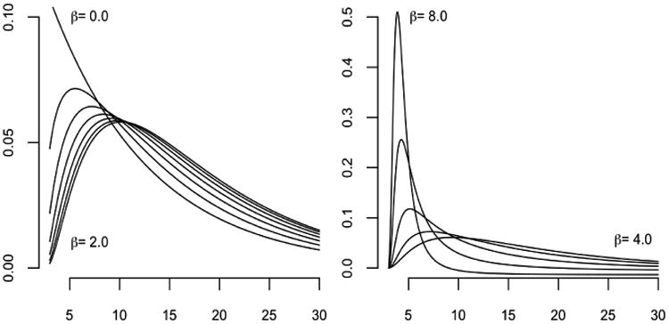
Conditional density of survival time for various values of β.

The conditional survival distribution given Y[t^(k)] depends not only on the current or most recent value, but on the entire vector. In particular, the conditional distribution does not have the structure of a regression model in which the longitudinal variable enters as a time-dependent covariate without temporal interference. Thus, on the assumption that the joint model is adequate, issues related to covariate confounding do not arise.

Figure 1 also shows convergence in the conditional densities for times sufficiently past the final observation time (t = 3); this behavior represents the weak dependence of the predictive distribution on measurements made sufficiently far in the past. In this example, the observed health-status values at appointment times t yield negligible information compared to the knowledge that the individual has survived well into the future.

4.2 Prediction under the latent-variable model

Consider the latent-variable model presented in Section 2. The joint density of (T, t^(k), Y[t^(k)]) at (t, t^(k), y) is again a product of three factors:

$$\begin{array}{c}\prod _{j<k}p(t_j,y_j|{\mathcal{H}}_j)\times f(t|{\mathcal{H}}_k)\\ =\prod _{j<k}p(y_j|{\mathcal{H}}_j)\times \prod _{j<k}p(t_j|{\mathcal{H}}_j)\times f(t|{\mathcal{H}}_k),\end{array}$$ (6)

Unlike equation (4), only the final factor depends on t; however, this component is conditional on the entire observed history and therefore ℋ_k is informative for survival prediction. Under a shared-random effects model (Rizopolous, 2012), the immortal process for patient i, m_i(t), is given by

$$E(m_i(t)|b_i;\beta )=x_i{(t)}^{\prime }\beta +z_i{(t)}^{\prime }{b}_i$$ (7)

with β and b_i denoting fixed and random effects respectively. For the latent-variable model given by equations (2) and (7), the conditional survival distribution given health records (t^(k), Y[t^(k)]) is

$$\text{pr}(T_i\ge u|{\mathbf{t}}^{(k)},Y[{\mathbf{t}}^{(k)}])=\int \frac{S_i(u|{\mathcal{M}}_i(u,b_i,\beta );\theta )}{S_i(t_{k-1}|{\mathcal{M}}_i(t_{k-1},b_i,\beta );\theta )}\cdot \text{pr}(b_i|{\mathbf{t}}^{(k)},Y[{\mathbf{t}}^{(k)}])d{b}_i$$

where θ denotes the set of survival parameters in equation (2), and ℳ_i(t, b_i, β) the entire expected health trajectory up to time t (i.e. {E(m_i(s) | b_i; β) | s ∈ [0, t)}). The conditional survival distribution is therefore a complex function of the entire health trajectory. Inadequate models for the health trajectory, including unobserved time points, could yield inaccurate survival predictions. In most survival studies, noisy health measurements are common making discovery of the “true” trajectories difficult if not impossible. Equation (4), on the other hand, is only a function of the observed patient history and does not require estimation of the unobserved components of the health trajectory. In the latent-variable model, how new measurements affect the conditional distribution is not obvious as the observed health trajectory enters in entirely. Finally, even with adequate models for the entire health trajectory, the predictive density has high computational complexity as compared with equation (4).

4.3 Illustration by simulation

Figure 2 shows simulated data for 200 patients whose survival times are independent exponential with mean five years. While the patient lives, annual appointments are kept with probability 5/(5 + t), so appointment schedules in the simulation are not entirely regular. Health status is a real-valued Gaussian process with mean E(Z(s)) = 10+10s/(10+s) in reverse time, and covariances

Fig. 2. Simulated health status sequences aligned by recruitment time (left) and the same sequences aligned by failure time (right).

$$cov(Z(s),Z(s^{\prime }))=(1+exp(-|s-s^{\prime }|/5)+{\delta }_{s{s}^{\prime }})/2$$

for s, s′ > 0, so there is an additive patient-specific effect in addition to temporal correlation. Values for distinct patients are independent and identically distributed. This distribution is such that health-status plots in reverse time aligned by failure show a stronger temporal trend than plots drawn in the conventional way. The state of health is determined more by time remaining before failure than time since recruitment. These trends could be accentuated by connecting successive dots for each individual, as in Fig. 2 of Sweeting and Thompson (2011), but this has not been done in Fig. 2.

Since the survival times are exponential with mean five, independent of covariates and treatment, the root mean squared prediction error using co-variates only is five years. For fixed k ≥ 2, and a patient having at least k appointments, the conditional survival distribution given the first k health-status values has a standard deviation depending on the observed configuration, but the average standard deviation is about 1.4 years, and the root mean squared prediction error is about 1.7 years. Using only the appointment schedule as a lower bound on the survival time, the root mean squared prediction error is 3.9 years. For this setting, the longitudinal variable is a reasonably effective predictor of survival, and the prediction error is almost independent of k in the range 2–5. This summary does not tell the full story because certain y-configurations lead to very precise predictions whereas others lead to predictive distributions whose standard deviation exceeds five years.

The parameter settings used in this simulation may not be entirely representative of the range of behaviours of the conditional survival distribution given Y[t]. If the ratio of the between-patient to within-patient variance components is increased, the average variance of the conditional survival distribution decreases noticeably with k. For such settings, prediction using the entire health history is more effective than prediction using the most recent value.

4.4 Recurrent health-related events

In certain circumstances the health outcome Y is best regarded as a point process, recording the occurrences of a specific type of non-fatal event, such as epileptic or asthmatic attacks or emergency-room visits. In other words, Y_i ⊂ R is the set of times at which patient i experiences the event. Then t = (0, t_k) is a bounded interval, and the observation Y[t] = Y ⋂ t is the set of events that occur between recruitment and the most recent appointment. This observation records the actual date of each event, which is more informative than the counting process #Y[(0, t₁)], …, #Y[(0, t_k)] evaluated at the appointment dates. If there are recurrent events of several types, Y is a marked point process, and Y[t] is the set of all events of all types that occur in the given temporal interval. The paper Schaubel and Zhang (2010) is one of several papers in the October 2010 issue of Lifetime Data Analysis, which is devoted to studies of this type.

In this situation, the frequency of the recurrent event may be constant over time, or it may vary in a systematic way. For example, the frequency may increase slowly but systematically as a function of either age or time since recruitment. Alternatively, the frequency may be unrelated to age at recruitment, but may increase in the last year of life as death approaches. In the former case, alignment of records by failure time is ineffective; in the latter case, the revival processes for different individuals have a common pattern, and alignment by failure tine is an effective device for exploiting this commonality.

We consider here only the simplest sort of recurrent-event process in which the revival process is Poisson, there is a single event type, and the subset Y ⋂ t = y of observed event times is finite. The mean measure of the revival process is Λ, which is non-atomic with intensity λ on the positive real line. The density ratio at t > sup(t) is the probability density at the observed event configuration t – y as a subset of the reverse-time interval t – t, i.e.,

$$g(\mathbf{y};t-\mathbf{t})=exp(-\Lambda (t-\mathbf{t}))\prod _{y\in \mathbf{y}}\lambda (t-y).$$

In particular, if the intensity is constant for s > 0, the density ratio is constant, and the event times are uninformative for survival. In other words, it is the temporal variation of the intensity function that makes the observed configuration y informative for patient survival.

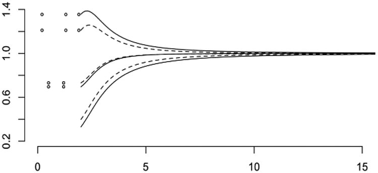
For a specific numerical example, let λ(s) = (2 + s²)/(1 + s²) be the revival intensity, and let t = (0, 2) be the observation window. The revival intensity, monotone decreasing with an asymptote of one, implies that the recurrent events are moderately common at all ages, but their frequency increases as failure approaches. Figure 3 shows the likelihood as a function of t ≥ 2 for three event configurations, y₀ = ø, y₁ = {0.5, 1.2} and y₂ = {0.2, 1.3, 1.9}. Since the likelihood function is defined only up to an arbitrary multiplicative constant the curves have been adjusted so that they are equal at t = 20 or effectively at t = ∞. In place of the predictive survival distributions we show instead the ratio of the predictive hazard functions to the marginal hazards as dashed lines on the assumption that the marginal failure distribution is exponential with mean 5. Because of the form of the revival intensity, which is essentially constant except near the origin, the predictive hazard functions are very similar in shape to the likelihood functions. Figure 3 illustrates again the weak dependence of the predictive distribution on measurements made sufficiently far in the past.

Fig. 3. Likelihood functions (solid lines) for three point configurations, with predictive hazard ratios (dashed lines).

4.5 Appointment schedule under sequential conditional independence

As discussed in Section 3.3, the appointment schedule is informative of survival. Ignoring the associated measurements recorded at appointment times, the appointment schedule can be viewed as a recurrent health-related event process. Here, we consider the appointment schedule assuming sequential conditional independence (i.e., condition (3)). Under this assumption, we fit a Poisson point process model with conditional intensity depending on the observed history and survival time. For the CSL1 trial, we present evidence that, even when controlling for the known schedule behavior, the conditional intensity depends on the time until failure.

First, recall for the CSL1 trial that each patient has an initial appointment at t = 0. Subsequent to the initial appointment, visits were scheduled to take place after three months, six months, twelve months, and then once every year afterwards. However, the observed appointment schedules varied considerably from the planned appointment sequence. We ignore the initial appointment as this is mandatory. Let π(t | (T, t^(kt), Y[t^(kt)])) denote the conditional intensity given the observed history up to time t (i.e., (t^(kt),Y[t^(kt)])) and survival time T. We assume the appointment schedule is a Poisson point process with conditional intensity

$$log(\pi (t|(T,{\mathbf{t}}^{(k_t)},Y[{\mathbf{t}}^{(k_t)}])))={\alpha }_0+{\tau }_{\overline{a}(s)}+{\alpha }_1\frac{s}{s+\gamma }+r{(t)}^T\beta$$

for t < T where τ_ā(s) is the treatment indicator, s = T_i – t, and r(t) is a vector depending on t designed to capture the known appointment schedule behavior. Recall there are three scheduled appointments in the initial year and then a single appointment every year subsequently. We start by capturing this in a simple manner, setting r₁(t) = log(3) for t < 1 and log(1) for t ≥ 1. Thus the baseline intensity is set to one level in the first year and then adjusted to a different level in all subsequent years. The third term is inverse linear and captures the potential non-linear dependence on the time until failure. The probability of the appointment schedule t is then given by

$$exp(-{\int }_0^T\pi (t|(T,{\mathbf{t}}^{(k_t)},Y[{\mathbf{t}}^{(k_t)}])dt)\prod _{k=1}^{k_T}\pi (t_k|(T,{\mathbf{t}}^{(k)},Y[{\mathbf{t}}^{(k)}]))$$

where k_t denotes the number of appointments before time t, and t_k denotes the kth appointment time. We approximate the integral with a sum by assuming the intensity function is piecewise constant on each day. We construct the conditional log-likelihood only for participants with uncensored records. The denominator term γ in all subsequent calculations is set at γ̂ = 0.01 years. Table 3 presents likelihood estimates along with standard errors for r(t) = r₁(t).

Table 3. Fitted coefficients for appointment schedule model.

	Altering baseline			Self-correcting
Covariate	Coef.	S.E.	Ratio
Intercept	3.97	0.13	29.86	4.10	0.14	29.74
s/(s + 0.01)	−3.86	0.14	−28.43	-3.95	0.14	-28.62
r1(t)	0.63	0.01	81.84	1.04	0.05	18.96
r2(t)	-	-	-	0.24	0.02	12.83
Prednizone	−0.04	0.05	−0.72	−0.03	0.05	−0.58

One may argue that this model does not capture the self-correcting nature of the appointment schedule. That is, if an appointment has yet to occur within the year then the patient is very likely to show up; however, if the appointment has already occurred, the patient is likely to not return until the next year. We can capture this by adding a second term into r(t) to account for the self-correcting nature of the appointment schedule. We set

$$r_2(t)=(t-1/3\cdot N^a[\lfloor t\rfloor ,t))\mathbf{1}[t\le 1]+(t-N^a[\lfloor t\rfloor ,t)\mathbf{1}[t>1]$$

where N^a[s, t) is the number of appointments within the window [s, t). The choice derives from work on self-correcting point processes of Isham and Westcott (1970). The process is self-correcting in that, if the appointment schedule strays too far from the target (3(t – ⎿t⏌) for the first year and (t – ⎿t⏌) in the second), then the intensity of the process compensates. Then we set r(t)^T = (r₁(t), r₂(t)). Table 3 presents likelihood estimates for this point process. Both models show that even when controlling for the appointment schedule behavior, the conditional intensity of the next appointment time depends on time until failure.

5 Parameter estimation

5.1 Likelihood factorization

The joint density for the observations in a revival model factors into two parts, one involving only survival times, the other involving only the revival process. More generally, the second factor is the conditional distribution of the revival process given T = t, so both factors depend on t. Although both factors may involve the same covariates and treatment indicators, the parameters in the two parts are assumed to be unrelated, i.e., variation independent. Thus the likelihood also factors, the first factor involving only survival parameters such as hazard modifiers associated with treatment and covariates, the second factor involving only health-status parameters such as temporal trends and temporal correlations. In other words, the two factors can be considered separately, either for maximum likelihood estimation or for Bayesian operations.

This approach is related to pattern-mixture modeling as discussed in Fieuws et al. (2008) in which the joint density pr(T, Y) is factorized as pr(Y | T) pr(T). Therefore the revival model can be viewed as a particular choice of pattern-mixture model. Initial contributions to the pattern-mixture approach include Little (1993) in the context of longitudinal clinical trials with dropout.

5.1.1 Survival distribution specification

The first stage in parameter estimation is to estimate the survival distribution F together with treatment and covariate effects if needed. Whether the model for survival times is finite-dimensional or infinite-dimensional, this step is particularly simple because the first factor involves only the survival times (censored and uncensored) and the survival distribution. The standard assumption of independent survival times for distinct patients simplifies the problem even further. Exponential, gamma and Weibull models are all feasible, with treatment effects included in the standard way.

For the Cox proportional-hazards model, the situation is more complicated. First, the survival time is finite with probability one if and only if the integrated hazard $\Lambda (R^{+})={\int }_0^{\infty }\lambda (t)dt$ is infinite, which is not satisfied at all parameter points in the model. Second, the partial likelihood function depends only on baseline hazard values λ(t) in the range 0 ≤ t ≤ T_max, where T_max is the maximum observed survival time, censored or uncensored. Thus, the likelihood does not have a unique maximum, but every maximum has the property that λ̂(t) = 0 for all 0 ≤ t ≤ T_max except for failure times, at which λ̂ has a discrete atom.

By common convention (Kaplan and Meier 1958; Cox 1972, §8) λ̂(t) = 0 for t > T_max, but this choice is not dictated by the likelihood function. Since the revival model requires survival times to be finite with probability one, it is essential to restrict the space of hazards to those having an infinite integral, which rules out the standard convention for λ̂. Equivariance under monotone temporal transformation points to a mathematically natural choice λ̂(t) = ∞ for t > T_max; a less pessimistic option is to use a finite non-zero constant such as

$$\widehat{\lambda }(t)=\frac{\text{total number of failures}}{\text{total person time at risk}}$$ (8)

for t > T_max. Both of these maximize the proportional-hazards likelihood function—restricted or unrestricted—and either one may be used in the revival model.

A less arbitrary alternative is to consider the set of neutral to the right processes (Kalbfleisch (1978), Clayton (1991), and Hjort (1990)). Such processes are exchangeable survival process constructed by generating survival times conditionally independent and identically distributed via a completely independent hazard measure, i.e. the cumulative conditional hazard is a Lévy process. These automatically satisfy the property that the survival time is finite with probability one. Anonymous (2015) show a correspondence with Markov survival processes, studying in particular the harmonic process for which the conditional distributions have a close affinity with the Kaplan-Meier estimator. For exchangeable survival times, the harmonic process is defined by two non-negative parameters, (ρ, ν). The marginal survival time is exponential with rate ν · (ψ(1 + ρ) – ψ(ρ)) where ψ is the derivative of the log gamma function. Given unique survival times T₁ < … < T_k the conditional hazard is the product of a continuous and discrete component. The continuous component is

$$H(t)=\sum _{i:T_i\le T}\nu \frac{T_i-T_{i-1}}{R^{\#}(T_{i-1})}+\nu \frac{T-T_j}{R^{\#}(T_j)+\rho },$$

where R^#(t) is the number of at risk individuals at time t−. The sum runs over survival times, both censored and uncensored, such that T_i ≤ T, and T_j is the last such time. The discrete component is a product over uncensored survival times

$$\prod _{j:T_j\le t,{\Delta }_j=0}\frac{r_j+\rho }{r_j+d_j+\rho }.$$ (9)

For small ρ, the discrete component is essentially the same as the right-continuous version of the Kaplan-Meier product limit estimator. The hazard rate for t > T_max is constant, λ = ν/ρ. Given ρ, the maximum likelihood estimate for λ is

$${[\frac{\rho }{k}{\int }_0^{\infty }(\psi (\rho +R^{\#}(t))-\psi (\rho ))dt]}^{-1}$$

As ρ tends to zero, the maximum likelihood estimate is non-unique. In particular, λ̂ is either 0 (i.e., equivalent to the common convention) or Σ_j(1 – Δ_j)/T_max. For ρ → ∞, the estimate approaches equation (8). Appendix B derives the estimators as ρ tends to zero when the marginal survival times are assumed to be distributed Weibull.

The harmonic process has both a simple form for the joint density and is easy to generate sequentially. Moreover, it is the only non-trivial Markov survival process with predictive distributions that are weakly continuous as a function of the initial configuration. The only exception is the iid process, which arises as the limit ρ → ∞ in which tied failures occur with probability zero. Given the above, it is a natural choice when working with the revival process. Inclusion of covariates is relatively straightforward and is discussed by Anonymous (2015).

5.1.2 Revival process specification

The second stage, which is to estimate the parameters in the revival process, is also straightforward, but only if all records are complete with no censoring. Serial dependence is inevitable in a temporal process, and there may also be independent persistent idiosyncratic effects associated with each patient, either additive or multiplicative. Gaussian revival models are particularly attractive for continuous health measurements because such effects are easily accommodated with block factors for patients and temporal covariance functions such as those included in the simulation in Fig. 2.

Thus the second stage involves mainly the estimation of variance components and range parameters in an additive Gaussian model. One slight complication is that the revival process is not expected to be stationary, which is a relevant consideration in the selection of covariance functions likely to be useful. Another complication is that the health status may be vector-valued, Y(t) ∈ R^q, so there are also covariance component matrices to be estimated. If the covariance function is separable, i.e.

$$cov(Z_{ir}(s),Z_{i{r}^{\prime }}(s^{\prime }))={\sum }_{r,r^{\prime }}K(s,s^{\prime })$$

for some q × q matrix Σ, maximum-likelihood estimation is straightforward. But separability is a strong assumption implying that temporal correlations for all health variables have the same pattern, including the same decay rate, which may not be an adequate approximation. Nevertheless, this may be a reasonable starting point.

The second stage requires all health records to be aligned at their termini. Accordingly, a record that is right censored (T_i > c_i so Δ_i = 1) cannot be properly aligned. If the complete records are sufficiently numerous, the simplest option is to ignore censored records in the second stage, on the grounds that the estimating equations based on complete records remain unbiased. This conclusion follows from the fact that the second factor is the conditional distribution given survival time. Thus, provided that the censoring mechanism is a selection based on patient survival time, the estimating equations derived from complete records are unbiased. The inclusion of censored records is thus more a matter of statistical efficiency than bias, and the information gained from incomplete records may be disappointing in view of the additional effort required. Note, likelihood estimates derived from complete records are unbiased under sequential conditional independence (i.e., condition (3)).

While alignment by death allows the revival model to incorporate important terminal behavior, this does not preclude the inclusion of initial behavior (i.e., the use of time since recruitment as a covariate). In section 6, the revival model depends on both the time until failure s = T – t and the survival time T. Therefore, the model indirectly depends on time since recruitment (i.e., re-write β₀T_i + β₁s as ${\beta }_0^{\text{'}}{T}_i+{\beta }_1^{\text{'}}t$ where ${\beta }_0^{\text{'}}={\beta }_0+{\beta }_1$ and ${\beta }_1^{\text{'}}=-{\beta }_1$. The inclusion of the null level also captures some behavior near onset of treatment. Moreover, deviations from the proposed revival model can be investigated. For example, we may check whether health sequences exhibit a trend associated with time measured from recruitment. We do this by including the generalized Brownian-motion covariance function −|t – t′| in the covariance model. Likelihood ratio tests can then be used to test whether there is significant characteristic patterns that are continuous in time measured from recruitment.

5.2 Incomplete records

If we choose to include in the likelihood the record for a patient censored at c > 0, we need the joint probability of the event T > c, the density of the subset t_c = t ⋂ [0, c], and the outcome Y[t_c] at y. On the assumption that censoring is uninformative, i.e., that the distribution of the subsequent survival time for a patient censored at time c is the same as the conditional distribution given T > c for an uncensored patient, the joint density is

$${\int }_{t\ge c}f(t)p({\mathbf{t}}_c|t)g(y;t-{\mathbf{t}}_c)dt$$

on the space of finite-length records. Assumption (5) implies that the second factor, the density of the appointment dates in [0, c] for a patient surviving to time t > c, does not depend on the subsequent survival time t – c, in which case it may be extracted from the integral. It is also reasonable to assume that the distribution of appointment schedules is known, for example if appointments are scheduled administratively at regular intervals, in which case the second factor may also be discarded. Since the survival probability 1 – F(c) is included in the first-stage likelihood, the additional likelihood factor needed in the analysis of the revival model is

$$\frac{1}{1-F(c)}{\int }_{t>c}f(t)g(y;t-{\mathbf{t}}_c)dt,$$

in which t_c may regarded as a fixed subset of [0, c]. Unfortunately, the integral involves both the survival density f(t) = F′(t) and the density of the revival process, so the full likelihood no longer factors. For an approximate solution, f may be replaced with the estimate obtained from the first-stage analysis of survival times, and if f̂ is purely atomic, the integral is converted to a finite sum.

For an incomplete record, the component of the derivative of the log-likelihood with respect to revival parameters, ψ, associated with the censored record (Y[t^(k)], t^(k), c) is

$$E_{\psi ,\theta }[\frac{dlogg(y;t-{\mathbf{t}}_c;\psi )}{d\psi }|(Y[{\mathbf{t}}_c],{\mathbf{t}}_c),T>c]$$

where θ denotes the survival parameters assumed common to both. This is the expected value of the score given the observed censored record and censoring time. Treating the survival time as missing data, a simple imputation method is proposed for approximate maximum likelihood estimation. First, impute survival times, T′, using the conditional survival distribution

$$f(T|(Y[{\mathbf{t}}_c],{\mathbf{t}}_c),T>c;{\widehat{\psi }}_u,\widehat{\theta })\propto f(T;\widehat{\theta })g(Y[{\mathbf{t}}_c];T-{\mathbf{t}}_c,{\widehat{\psi }}_u)\cdot \mathbf{1}[T>c]$$

where ψ̂_u is the maximum likelihood estimate of the revival parameters for uncensored records, and θ̂ the maximum likelihood estimate of the survival parameters using both uncensored and censored records.

In this case the log-likehood component associated with the imputed, un-censored record is given by

$$logg(y;T^{\prime }-{\mathbf{t}}_c;\psi )+logf(T^{\prime };\theta ),$$

so parameter estimation after imputation is again straightforward. Imputation performed multiple times creates imputed estimates { ${\widehat{\psi }}_1^{(I)},\dots ,{\widehat{\psi }}_M^{(I)}$} with standard errors { $s_1^{(I)},\dots ,s_M^{(I)}$}. These can then be averaged to get a complete-data estimate, $\widehat{\psi }=\frac{1}{M}{\sum }_{m=1}^M{\psi }_m^{(I)}$. A variance estimate, V_ψ reflects variation within and between imputations:

$$V_{\psi }=W+(1+\frac{1}{m})B$$

where $W=\frac{1}{M}\sum s_m^2$ and $B=\frac{1}{M-1}{\sum }_{m=1}^M{({\widehat{\psi }}_m-\widehat{\psi })}^2$. Let, ${\widehat{\psi }}_{\text{imp}}^{(c)}$ denote the estimate for the censored records under imputation of the survival times.

Given maximum likelihood estimates, ψ̂^(c) and ψ̂^(u), and corresponding standard errors, V̂^c and V̂^u, the following statistic is proposed for testing whether censored records are consistent with uncensored records:

$$T_i=\frac{{\widehat{\psi }}_i^{(c)}-{\widehat{\psi }}_i^{(u)}}{\sqrt{{({\widehat{V}}_i^c)}^2+{({\widehat{V}}_i^u)}^2}}$$ (10)

The denominator is the estimated variance of the difference under independence of the patients' revival processes. While equation (10) can be used, when the survival times are imputed the estimates, ψ̂^(u) and ${\widehat{\psi }}_{\text{imp}}^{(c)}$, are positively correlated as the imputed survival times use the maximum likelihood estimate for uncensored records, resulting in a conservative test statistic.

A Monte-Carlo EM algorithm for exact likelihood analysis with incomplete records was investigated. This is technically more involved, but omitted as imputation provides similar estimates in the data considered here. The situation is considerably more complicated if the revival processes for distinct patients are not independent.

5.3 Treatment effect: definition and estimation

We consider here only the simplest sort of revival model for the effect of treatment on patient health, ignoring entirely its effect on survival time. Health status in the revival process is assumed to be Gaussian, independent for distinct patients, and the treatment is assumed to have an effect only on the mean of the process, not on its variance or covariance. Consider two patients, one in each treatment arm,

$$\begin{array}{cc}{a}_i(t)={\overline{a}}_i(T_i-t)=1,& a_j(t)={\overline{a}}_j(T_j-t)=0\end{array}$$

such that x_i = x_j. If Z is independent of T, then the random variable Z_i(s) – Z_j(s) is distributed independently of the pair T_i, T_j. By definition, the treatment effect as defined by the revival model is the difference of means

$${\tau }_{10}(s)=E(Z_i(s))-E(Z_j(s))=E(Y_i(T_i-s))-E(Y_j(T_j-s))$$

at revival time s. This is not directly comparable with either of the the conventional definitions

$$\begin{array}{ccc}{\gamma }_{10}(t)=E(Y_i(t)-E(Y_j(t))& \text{or}& {\gamma }_{10}^{\text{'}}(t)=E(Y_i(t)-E(Y_j(t)|T_i,T_J>t)\end{array}$$

in which the distributions are compared at a fixed time following recruitment. The expectation in a survival study—that healthy individuals tend to live longer than the frail—implies that E(Y(t) | T) must depend on the time remaining to failure. In that case, the conventional treatment definition ${\gamma }_{10}^{\text{'}}(t)$ depends explicitly on the difference between the two survival times. In other words, it does not disentangle the effect of treatment on patient health from its effect on survival time.

If Z is not independent of T but the dependence is additive, the difference of means at revival time s

$$E(Z_i(s)|T)=E(Z_j(s)|T)={\tau }_{10}(s)+\gamma (T_i)-\gamma (T_j)$$

contains both a treatment effect and an effect due to the difference in survival times. In other words, the fact that Z and T are not independent does not necessarily complicate the interpretation of treatment effects. By contrast with standard practice in the analysis of randomized trials with longitudinal responses, (Fitzmaurice, Laird and Ware 2011, section 5.6), it is most unnatural in this setting to work with the conditional distribution given the baseline outcomes Y_i(0) ≡ Z_i(T_i). This is one reason why the baseline response should be regarded as an integral part of the outcome sequence, not as a covariate. Exchangeability implies distributional equality Z_i(T_i) ∼ Z_j(T_j) for individuals having the same covariate values, but it does not imply equality of conditional distributions given T. On the presumption that treatment assignment is independent of baseline response values, we also have Z_i(T_i) ∼ Z_j(T_j) conditionally on treatment, whether or not a_i, a_j are equal. Consequently, in order to satisfy the exchangeability assumption, it is necessary to introduce a null, pre-randomization, treatment level, a_i(0) = a_j(0), common to all subjects.

6 A worked example: cirrhosis study

6.1 Prednizone and prothrombin levels

In the period 1962–1969, 532 patients in Copenhagen hospitals with histologically verified liver cirrhosis were randomly assigned to two treatment arms, control and prednisone. Only 488 patients for whom the initial biopsy could be reevaluated using more restrictive criteria were retained, yielding 251 and 237 patients in the prednisone and placebo groups respectively. Variables recorded at entry include sex, age, and several histological classifications of the liver biopsy. Clinical variables were also collected, including information on alcohol consumption, nutritional status, bleeding, and degree of ascites. However, these covariates were not included in the dataset used here, which was downloaded from the R library http://cran.r-project.org/web/packages/joineR maintained by Philipson Sousa, Diggle, Williamson, Kolamunnage-Dona and Henderson. At the end of the study period, the mortality rate was 292/488, or approximately 60%.

The focus here is on the prothrombin index, a composite blood coagulation index related to liver function, measured initially at three-month intervals and subsequently at roughly twelve-month intervals. The individual prothrombin trajectories are highly variable, both in forward and in reverse time, which tends to obscure patterns and trends. In Figure 4a the mean trajectory is plotted against time from recruitment for two patient groups placebo/prednisone and censored/not censored. Naturally, only those patients who are still alive are included in the average for that time. Figure 4b shows the same plots in reverse alignment. While there are certain similarities in the two plots, the differences in temporal trends are rather striking. See Appendix H for details on estimation of both mean trajectories. In particular, prothrombin levels in the six months prior to censoring are fairly stable, which is in marked contrast with levels in the six months prior to failure, as seen in the lower pair of curves. As values of the prothrombin index above seventy are considered normal, it is not unreasonable for the trajectories in the six months prior to failure to drop below this threshold.

Inspection of the graphs for uncensored patients in the right panel of Figure 4 suggests beginning with the simplest revival model in which the sequences for distinct patients are independent Gaussian with moments

$$\begin{array}{c}E(Z_i(s)|T)=\alpha +{\tau }_{{\overline{a}}_i(s)}+{\beta }_0{T}_i+{\beta }_{1}s+{\beta }_{2}log(s+\delta )\\ cov(Z_i(s),Z_j(s^{\prime })|T)={\sigma }_1^2{\delta }_{ij}{K}_1(s,s^{\prime })+{\sigma }_2^2{\delta }_{ij}+{\sigma }_3^2{\delta }_{ij}{\delta }_{s{s}^{\prime }}.\end{array}$$

The non-linear dependence on s is accommodated by the inclusion of log(s + δ) in the mean model with a temporal offset δ, which is equal to one day in all subsequent calculations. Inclusion of the survival time T_i is suggested by the increasing trend along the diagonals and sub-diagonals of Table 1. Since the value at recruitment is included as a response for each series, treatment necessarily has three levels, null, control and prednisone. The three covariance terms are associated with independent additive processes, the second for independent and identically distributed patient-specific constants, and the third for independent and identically distributed white noise or measurement error. The first covariance term governs the prothrombin sequences for individual patients, which are assumed to be continuous in time with covariance function K₁(s, s′) = exp(−|s – s′|/λ) for s, s′ > 0. The temporal range in all subsequent calculations is set at λ̂ = 1.67 years, implying an autocorrelation of 0.55 at a lag of one year. The implied one-year autocorrelation for the observed prothrombin sequences is considerably smaller, roughly 0.30, because of the white-noise measurement term.

For the initial likelihood calculations that follow, incomplete records are ignored; only the 1634 measurements for the 292 non-censored patients are used. The fitted variance components, estimated by maximizing the residual likelihood, are

$$({\widehat{\sigma }}_1^2,{\widehat{\sigma }}_2^2,{\widehat{\sigma }}_3^3)=(210.0,206.8,179.6),$$

all significantly positive. Using these values to determine the covariance matrix, the weighted least-squares coefficients in the mean model are shown in Table 4. The standard error for the prednisone/control contrast is 1.77, somewhat larger than the standard error for the prednisone/null contrast because the former is a contrast between patients involving all three variance components, whereas the latter is a contrast within patients, which is unaffected by the second variance component. Recall these likelihood estimates are unbiased under the sequential conditional independence assumption (condition (3)).

Table 4. Fitted coefficients for revival model.

	Censored Records			Uncensored Records
Covariate	Coef.	S.E.	Ratio	Coef.	S.E.	Ratio
Null Treatment	0.00	-	-	0.00	-	-
Control	4.13	1.84	2.3	2.41	1.43	1.7
Prednizone	11.56	1.75	6.6	13.55	1.47	9.2
Survival (T)	2.65	0.39	6.9	1.75	0.47	3.7
Revival (s)	−2.78	0.49	−5.7	−2.11	0.47	−4.5
log(s + S)	3.74	2.68	1.4	4.66	0.41	11.5
λ				0.164

Various deviations from this initial model may now be investigated. In particular, it is possible to check whether there is an interaction between treatment and survival time, i.e., whether the treatment effect for long-term survivors is or is not the same as the treatment effect for short-term survivors. This comparison involves two variance-components models having different mean-value subspaces, so the residual likelihoods are not comparable. For likelihood comparisons, the kernel subspace must be fixed, and the natural choice is the mean-value subspace for the null model as described by Welham and Thompson (1997) or as implemented by Clifford and McCullagh (2006). The likelihood ratio statistic computed in this way is 0.83 on two degrees of freedom, showing no evidence of interaction. However, there is appreciable evidence in the data that the treatment effect (prednisone versus control) decreases as t → T, i.e., as s → 0. The likelihood-ratio statistic for the treat.s interaction is 3.90 on two degrees of freedom, showing little evidence of a linear trend, but the value for the treat. log(s) interaction is 8.68, pointing to a non-linear trend.

We may also check the adequacy of the assumed form for the mean model by including an additional random deviation, continuous in reverse time, with generalized non-stationary covariance function such as K₀(s, s′) = −| log(s + δ) – log(s′ + δ)|. The fitted coefficient is 2.38, and the associated likelihood ratio statistic is 1.2 on one degree of freedom, showing no significant deviations that are continuous in reverse time. Finally, we check whether the sequences for different patients exhibit a characteristic pattern or trend associated with time measured from recruitment by including the generalized Brownian-motion covariance function −|t –t′| in the covariance model. The fitted variance coefficient is 2.10, and the likelihood ratio statistic is 2.38 on one degree of freedom showing no significant characteristic patterns that are continuous in time measured from recruitment.

Using the imputation method proposed in section 5.2, revival parameters for censored records are estimated in order to check consistency with uncensored records. We initially considered the marginal survival time to be exponential with rate dependent on treatment which was the only available baseline variable. However, the treatment indicator was statistically insignificant. This analysis, along with a similar analysis under weibull and Cox-proportional hazards specifications, are reported in the supplementary material. For this reason, we start by assuming the marginal survival time is exponential with rate parameter given by the first stage maximum likelihood estimate. We assume the appointment schedule is uninformative (i.e., condition (5)); survival times are then imputed. The imputation estimates are shown in Table 4. Standard errors of coefficients that do not depend on the behavior near the origin of the revival times are similar to those for uncensored records. Not surprisingly, the standard error for log(s + δ) is substantially higher for censored records. The parameters associated with the survival and revival times show some deviation across record type, while treatment effects and the non-linear behavior with respect to the revival time appear consistent. Conclusions appear robust to survival distribution specification as shown in Appendices C and D, where imputed estimates under both exponential and Weibull specifications for the above model as well as that including an interaction with treatment are provided.

A concern may be the parametric specification of the survival time distribution and whether this limits the method for handling censored records. To address this, Appendix B shows estimates under the Markov survival process specification when ρ is sent to zero. The result is a conditional survival distribution equivalent to the Kaplan-Meier product estimator for t < T_max. For t ≥ T_max the hazard function is the Weibull hazard function. Appendix E finds maximum likelihood estimates for the survival distribution parameters when the marginal survival times are assumed Weibull. We see that the estimated conditional distribution is approximately equivalent to assuming the hazard is infinite for all times after T_max = 13.40. Table 9 and 11 shows the imputed estimates are similar to those under the exponential specification.

An additional concern may be the assumption of an uninformative appointment schedule. To address this, we present imputed estimates under the self-correcting appointment schedule estimated in Section 4.5. Table 13 and 15 shows the imputed estimates are similar to those under the marginal exponential specification with uninformative appointment times.

6.2 Effect of prothrombin on prognosis

Over a period of 5 years and one month following recruitment, patient u had eight appointments with prothrombin values as follows:

tu (days)	0	126	226	392	770	1127	1631	1855
Yu[tu]	49	93	122	120	110	100	72	59

This is in fact the record for patient 402 who was assigned to prednisone and was subsequently censored at 2661 days. As determined on day 1855, the survival prognosis for this patient depends on preceding sequence of measurements. Relative to the unconditional survival density for a patient on the prednisone arm, the conditional survival density at time t > max(t_u) is modified multiplicatively by a factor proportional to the joint conditional density of the random variable Z_u[t – t_u] at the observed point y_u given T_u = t and the data observed for all other patients.

For the model described in the preceding section—in which the records for distinct patients are independent—this factor is particularly simple. The conditional distribution of Z_u[t–t_u] given T = t has a mean vector μ depending linearly on t –t_u and log(t − t_u + δ), and a covariance matrix Σ that is constant in t. The log density at y_u is a quadratic form

$$h(t,y_u)=\text{const}-{(y_u-\mu )}^{\prime }{\sum }^{-1}(y_u-\mu )/2$$

depending on t only through μ. This estimated factor is shown in Figure 5a for three versions of the record in which the final prothrombin value is 59, 69 or 79.

Fig. 5.

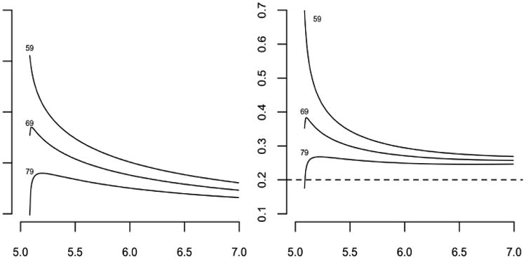
Three versions of the record for patient 402: log modification factors for the predictive survival density (left panel) and hazard functions (right panel).

It may be helpful to express the effect of the observed prednisone record on the conditional survival distribution through its effect on the hazard function at times t > max(t_u) rather than its effect on the conditional survival density. Suppose, therefore, that the unconditional survival time for a patient on the prednisone arm, is exponential with mean 5 years, so that the unconditional hazard function is constant. What is the conditional hazard at time t > max(t_u) given the prothrombin sequence for patient u, with no further measurements made in the interval (max(t_u), t) other than survival? The conditional hazard functions for the subsequent two-year interval 5 < t < 7 are shown in Fig. 5b for the same three versions of the prothrombin record. It is evident from these plots that the conditional hazard for the real patient is substantially elevated following the last measurement, but the effect is transient and does not persist for the duration of a typical inter-appointment interval of one year. If the final value were 79 instead of 59, the hazard function is almost constant, initially increasing and subsequently reverting to the long-term value, which is slightly larger than the unconditional hazard.

We also consider the effect of prothrombin on prognosis when accounting for the appointment schedule. We consider the estimated self-correcting appointment schedule model discussed in Section 4.5. We alter the log density estimates using the estimated coefficients in Table 3 and present the estimated factor in Figure 6a for the same three versions of the record. The conditional hazard functions for the subsequent two-year interval 5 < t < 7 are shown in Fig. 6b.

Fig. 6.

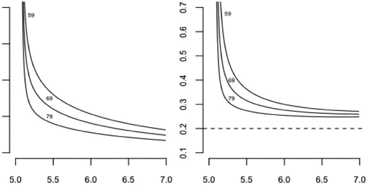
Three versions of the record for patient 402: log modification factors for the predictive survival density (left panel) and hazard functions (right panel) when accounting for the self-correcting appointment schedule distribution.

The preceding analyses indicates that it may be misleading to treat the observed health sequence as a time-dependent covariate in the proportional-hazards model. At any one failure time t measured from recruitment, some of the health measurements are recent and fresh, while others are likely to be up to one year old. Figure 5b shows that stale measurements may have negligible prognostic value. The predictive revival model automatically takes into account the time that has passed since the last appointment, so that stale values are discounted appropriately. For all three versions of the record for patient 48, the conditional hazard functions converge to the same long-term value.

Figure 7 plots three versions of the hazard function for patient 402 under the latent-variable model (Rizopolous, 2012) with linear fixed and random effects. In this case, hazard functions do not converge; instead the gap remains over the subsequent two years implying the conditional hazard function for this model depends heavily on the stale measurements.

Fig. 7.

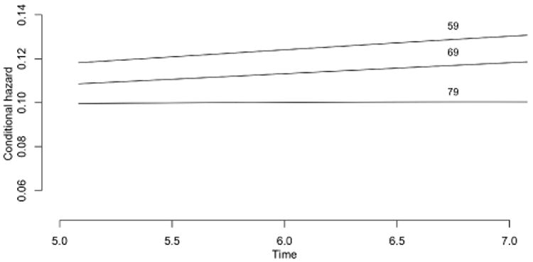
Hazard function for the latent-variable model for three versions of state for patient 402.

6.3 Review of assumptions

The conditional independence assumption (3) does not require appointments to be scheduled administratively, nor does it forbid patient-initiated appointments. Consider two patients i, j at time s prior to failure, having similar prior appointment schedules and similar health values. Assumption (3) states that the conditional appointment-initiation intensity given the observed health record and subsequent survival time does not depend on subsequent health values. In other words, conditional independence implies that patients i, j are equally likely to initiate an appointment at time s; it is also assumed implicitly that they do so independently.

The evidence presented in section 3.3, and in Liestøl and Andersen (2002) shows clearly that the rate of patient-initiated appointments increases in the last few months of life. It is certainly possible that patient behaviour in this instance violates the conditional independence assumption, but the evidence presented does not directly address the matter. All in all, assumption (3) seems unavoidable and relatively benign.

The non-informative assumption (5) is much stronger than (3). It implies that appointments are scheduled as if the patient will live indefinitely, which is clearly contradicted by the evidence in the CSL1 study. We now examine the consequences of failure of (5), retaining (3).

Assumption (3) implies that the sampling is non-preferential in the sense of Diggle, Menezes and Su (2010), which means that the second factor in (4) is the same as if the appointment dates had been fixed by design. Consequently, the likelihood calculations in section 5 are unaffected by the failure of (5).

If the appointment for patient u on day 1855 were self-initiated in such a way that the last factor in (4) depends on subsequent survival, it would be technically incorrect to omit that factor in prognosis calculations. However, if it were known that all appointments for patient u were on schedule, the possibility of a dependence on subsequent survival is eliminated, and the prognosis calculations for this patient is technically correct even if the behaviour of other patients violates (5).

7 Summary

The paper examines the problem of model formulation for health sequences, whose defining characteristic is that the state space contains an absorbing value. Each health sequence is terminated ultimately by death, which is not equivalent to random restriction or censoring because subsequent values are known. Typically, sequence length and sequence values are not independent.

The principal suggestion is that it may be more natural in some circumstances to align health sequences by failure time than by age or by recruitment date. The following list describes various statistical implications of realignment.

1. The health sequence is regarded as a random process in its own right, not as a time-dependent covariate governing survival.

2. To a substantial extent, the model for survival time is decoupled from the revival model for the behaviour of the health sequence in reverse time.

3. Realignment implies that value Y_i(0) at recruitment must not be treated as a covariate, but as an integral part of the response sequence. If they were available, values prior to recruitment could also be used.

4. The definition of a treatment effect is not the usual one because the natural way to compare the records for two individuals is not at a fixed time following recruitment, but at a fixed revival time. The treatment value need not be constant in revival time.

5. The predictive value of a partial health sequence for subsequent survival emerges naturally from the joint survival-revival distribution. In particular, the conditional hazard given the finite sequence of earlier values is typically not constant during the subsequent inter-appointment period. For times sufficiently far from in the future, the conditional hazard often exhibits weak dependence on such “stale measurements”.

6. Records cannot be aligned until the patient dies, which means that the revival process is not observable component-wise until T is known. As a result, the likelihood analysis for incomplete records is technically more complicated. An imputation method has been introduced for estimation with incomplete records.

7. The omission of incomplete records from the revival likelihood does not lead to bias in estimation, but it does lead to inefficiency, which could be substantial if the majority of records are incomplete.

8. The principal assumption, that appointment dates be uninformative for subsequent survival, does not affect likelihood calculations, but it does affect prognosis calculations for individual patients. For that reason, it is advisable to label all appointments as scheduled or unscheduled.

References

- Anonymous. Details omitted for double-blind reviewing 2015 [Google Scholar]
- Anonymous. Details omitted for double-blind reviewing 2016 [Google Scholar]
- Albert PS, Shih JH. An approach for jointly modeling multivariate longitudinal measurements and discrete time-to-event data. The Annals of Applied Statistics. 2010;4:1517–1532. doi: 10.1214/10-AOAS339. [DOI] [PMC free article] [PubMed] [Google Scholar]
- Andersen PK, Hansen LH, Keiding N. Assessing the influence of reversible disease indicators on survival. Statistics in Medicine. 1991;10:1061–1067. doi: 10.1002/sim.4780100706. [DOI] [PubMed] [Google Scholar]
- Chan K, Wang M. Backward estimation of stochastic processes with failure events as time origins. Ann Appl Stat. 2010;4:1602–1620. doi: 10.1214/09-AOAS319. [DOI] [PMC free article] [PubMed] [Google Scholar]
- Clayton DG. A Monte Carlo method for Bayesian inference in frailty models. Biometrics. 1991;47:467–485. [PubMed] [Google Scholar]
- Clifford D, McCullagh P. The regress function. R Newsletter. 2006;6:6–10. [Google Scholar]
- Crowther MJ, Andersson TM, Lambert PC, Abrams KR, Humphreys K. Joint modelling of longitudinal and survival data: incorporating delayed entry and an assessment of model misspecification. Statistics in Medicine. 35:1193–1209. doi: 10.1002/sim.6779. [DOI] [PMC free article] [PubMed] [Google Scholar]
- Cox DR. Regression models and life tables (with discussion) J Roy Statist Soc B. 1972;34:187–220. [Google Scholar]
- Cox DR, Snell EJ. Applied Statistics. London: Chapman and Hall; 1981. [Google Scholar]
- DeGruttola V, Tu XM. Modeling progression of CD-4 lymphocyte count and its relation to survival time. Biometrics. 1994;50:1003–1014. [PubMed] [Google Scholar]
- Diggle PJ, Heagerty P, Liang KY, Zeger SL. Analysis of Longitudinal Data. Oxford Science Publications: Clarendon Press; 2002. [Google Scholar]
- Diggle PJ, Farewell D, Henderson R. Analysis of longitudinal data with drop-out: objectives, assumptions and a proposal (with discussion) Applied Statistics. 2007;56:499–550. [Google Scholar]
- Diggle PJ, Sousa I, Chetwynd A. Joint modeling of repeated measurements and tome-to-event outcomes: The fourth Armitage lecture. Statistics in Medicine. 2008;27:2981–2998. doi: 10.1002/sim.3131. [DOI] [PubMed] [Google Scholar]
- Diggle P, Menezes R, Su TL. Geostatistical inference under preferential sampling (with discussion) Appl Statist. 2010;59:191–232. [Google Scholar]
- Ding J, Wang JL. Modeling longitudinal data with nonparamet-ric multiplicative random effects jointly with survival data. Biometrics. 2008;64:546–556. doi: 10.1111/j.1541-0420.2007.00896.x. [DOI] [PMC free article] [PubMed] [Google Scholar]
- Farewell D, Henderson R. Longitudinal perspectives on event history analysis. Lifetime Data Analysis. 2010;6:102–117. doi: 10.1007/s10985-009-9137-1. [DOI] [PubMed] [Google Scholar]
- Faucett CL, Thomas DC. Simultaneously modeling censored survival data and repeatedly measured covariates: a Gibbs sampling approach. Statistics in Medicine. 1996;15:1663–1685. doi: 10.1002/(SICI)1097-0258(19960815)15:15<1663::AID-SIM294>3.0.CO;2-1. [DOI] [PubMed] [Google Scholar]
- Fieuws S, Verbeke G, Maes B, Vanrenterghem Predicting renal graft failure using multivariate longitudinal profiles. Biostatistics. 2008;9:419–431. doi: 10.1093/biostatistics/kxm041. [DOI] [PubMed] [Google Scholar]
- Fitzmaurice GM, Laird NM, Ware JH. Applied Longitudinal Data Analysis. 2nd. New York: Wiley; 2011. [Google Scholar]
- Fitzmaurice G, Davidian M, Verbeke G, Molenberghs G. Longitudinal Data Analysis. Chapman & Hall; 2009. [Google Scholar]
- Guo X, Carlin B. Separate and joint modeling of longitudinal and event time data using standard computer packages. American Statistician. 2004;58:1–10. [Google Scholar]
- Henderson R, Diggle P, Dobson A. Joint modeling of longitudinal measurements and event time data. Biostatistics. 2000;1:465–480. doi: 10.1093/biostatistics/1.4.465. [DOI] [PubMed] [Google Scholar]
- Hjort NL. Nonparametric Bayes estimators based on beta processes in models for life history data. Annals of Statistics. 1990;18:1259–1294. [Google Scholar]
- Houwelingen HC. From model building to validation and back: a plea for robustness. Statistics in Medicine. 2014;33:5223–5238. doi: 10.1002/sim.6282. [DOI] [PubMed] [Google Scholar]
- Huang CY, Wang MC. Joint modeling and estimation for recurrent event processes and failure time data. Journal of the American Statistical Association. 2004;99:1153–1165. doi: 10.1198/016214504000001033. [DOI] [PMC free article] [PubMed] [Google Scholar]
- Isham V, Westcott M. A self-correcting point process. Stoch Processes Appl. 1970;8:335–347. [Google Scholar]
- Kalbfleisch JD. Nonparametric Bayesian analysis of survival time data. J Roy Statist Soc B. 1978;40:214–221. [Google Scholar]
- Kalbfleisch JD, Prentice RL. The Statistical Analysis of Failure Time Data. Hoboken, New Jersey: John Wiley & Sons, Inc; 2002. [Google Scholar]
- Kong S, Nan B, Kalbfleisch JD, Saran R, Hirth R. Conditional Modeling of Longitudinal Data With Terminal Event. Journal of the American Statistical Association. 2017;0:1–12. doi: 10.1080/01621459.2016.1255637. [DOI] [PMC free article] [PubMed] [Google Scholar]
- Kurland BF, Johnson LL, Egleston BL, Diehr PH. Longitudinal data with follow-up truncated by death: match the analysis method to the research aims. Statistical Science. 2009;24:211–222. doi: 10.1214/09-STS293. [DOI] [PMC free article] [PubMed] [Google Scholar]
- Lagakos SW. A stochastic model for censored-survival data in the presence of an auxiliary variable. Biometrics. 1976;32:551–559. [PubMed] [Google Scholar]
- Li L, Hu B, Greene T. A Semiparametric Joint Model for Longitudinal and Survival Data with Application to Hemodialysis Study. Biometrics. 2009;65:737–745. doi: 10.1111/j.1541-0420.2008.01168.x. [DOI] [PubMed] [Google Scholar]
- Li Z, Tosteson TD, Bakitas M. Joint modeling quality of life and survival using a terminal decline model in palliative care studies. Statistics in Medicine. 2013;32:1394–1406. doi: 10.1002/sim.5635. [DOI] [PMC free article] [PubMed] [Google Scholar]
- Li Z, Frost HR, Tosteson TD, Liu L, Lyons K, Chen H, Cole B, Currow D, Bakitas M. A semiparametric joint model for terminal trend of quality of life and survival in palliative care research. Statistics in Medicine. 2017;36:4692–4704. doi: 10.1002/sim.7445. [DOI] [PMC free article] [PubMed] [Google Scholar]
- Lee JC. Prediction and estimation of growth curves with special co-variance structures. J Amer Statist Assoc. 1988;83:432–440. [Google Scholar]
- Lee JC. Tests and model selection for the general growth curve model. Biometrics. 1991;47:147–159. [PubMed] [Google Scholar]
- Laird N. Longitudinal panel data: an overview of current methodology. In: Cox DR, Hinkley DV, Barndorff-Nielsen OE, editors. Time Series Models in Econometrics, Finance and Other Fields. Chapman & Hall Monographs on Statistics and Applied Probability; 1996. p. 65. [Google Scholar]
- Liestøl K, Andersen PK. Updating of covariates and choice of time origin in survival analysis: problems with vaguely defined disease states. Statistics in Medicine. 2002;21:3701–3714. doi: 10.1002/sim.1322. [DOI] [PubMed] [Google Scholar]
- Little RJA. Pattern-mixture models for multivariate incomplete data. Journal of the American Statistical Association. 1993;88:125–134. [Google Scholar]
- McCullagh P. Sampling bias and logistic models (with discussion) J Roy Statist Soc B. 2008;70:643–677. [Google Scholar]
- Murphy SA. Optimal dynamic treatment regimes (with discussion) J Roy Statist Soc B. 2003;25:331–366. [Google Scholar]
- Rizopoulos D. JM: An R package for the joint modeling of longitudinal and time-to-event data. Journal of Statistical Software. 2010;35:1–33. [Google Scholar]
- Rizopoulos D. Joint Models for Longitudinal and Time-to-Event Data. Chapman and Hall; 2012. [DOI] [PMC free article] [PubMed] [Google Scholar]
- Rosthøj S, Keiding N, Schmiegelow N. Estimation of dynamic treatment strategies for maintenance therapy of children with acute lymphoblastic leukaemia: an application of history-adjusted marginal structural models. Statistics in Medicine. 2012;31:470–488. doi: 10.1002/sim.4393. [DOI] [PubMed] [Google Scholar]
- Schaubel DE, Zhang M. Estimating treatment effects on the marginal recurrent event mean in the presence of a terminating event. Lifetime Data Analysis. 2010;16:451–477. doi: 10.1007/s10985-009-9149-x. [DOI] [PMC free article] [PubMed] [Google Scholar]
- Sweeting MJ, Thompson SG. Joint modeling of longitudinal and time-to-event data with application to predicting abdominal aortic aneurysm growth and rupture. Biometrical Journal. 2011;53:750–763. doi: 10.1002/bimj.201100052. [DOI] [PMC free article] [PubMed] [Google Scholar]
- Ten Have TR, Miller ME, Reboussin BA, James MK. Mixed effects logistic regression models for longitudinal ordinal functional response data with multiple-cause drop-out from the longitudinal study of aging. Biometrics. 2000;56:279–287. doi: 10.1111/j.0006-341x.2000.00279.x. [DOI] [PubMed] [Google Scholar]
- Tsiatis AA, DeGruttola V, Wulfsohn MS. Modeling the relationship of survival to longitudinal data measured with error: applications to survival and CD4 counts in patients with AIDS. J Amer Statist Assoc. 1995;90:27–37. [Google Scholar]
- Tsiatis AA, Davidian M. Joint modeling of longitudinal and time-to-event data: an overview. Statistica Sinica. 2004;14:809–834. [Google Scholar]
- van Houwelingen HC, Putter H. Monographs on Statistics and Applied Probability. CRC Press; 2012. Dynamic Prediction in Clinical Survival Analysis; p. 123. [Google Scholar]
- Welham SJ, Thompson R. Likelihood ratio tests for fixed model terms using residual maximum likelihood. J Roy Statist Soc B. 1997;59:701–714. [Google Scholar]
- Wulfsohn MS, Tsiatis AA. A joint model for survival and longitudinal data measured with error. Biometrics. 1997;53:330–339. [PubMed] [Google Scholar]
- Xu J, Zeger SL. Joint analysis of longitudinal data comprising repeated measures and times to events. Applied Statistics. 2001;50:375–387. [Google Scholar]
- Zeger SL, Liang KY. Longitudinal data analysis for discrete and continuous outcomes. Biometrics. 1986;42:121–130. [PubMed] [Google Scholar]
- Zeger SL, Liang KY, Albert P. Models for longitudinal data: a generalized estimating equation approach. Biometrics. 1988;44:1049–1060. [PubMed] [Google Scholar]
- Zeng D, Lin DY. Semiparametric Transformation Models With Random Effects for Joint Analysis of Recurrent and Terminal Events. Biometrics. 2009;65:746–752. doi: 10.1111/j.1541-0420.2008.01126.x. [DOI] [PMC free article] [PubMed] [Google Scholar]
Associated Data
This section collects any data citations, data availability statements, or supplementary materials included in this article.