Evaluating the Columnar Stability of Acoustic Processing in the Human Auditory Cortex

Abstract

Using ultra-high field fMRI, we explored the cortical depth-dependent stability of acoustic feature preference in human auditory cortex. We collected responses from human auditory cortex (subjects from either sex) to a large number of natural sounds at submillimeter spatial resolution, and observed that these responses were well explained by a model that assumes neuronal population tuning to frequency-specific spectrotemporal modulations. We observed a relatively stable (columnar) tuning to frequency and temporal modulations. However, spectral modulation tuning was variable throughout the cortical depth. This difference in columnar stability between feature maps could not be explained by a difference in map smoothness, as the preference along the cortical sheet varied in a similar manner for the different feature maps. Furthermore, tuning to all three features was more columnar in primary than nonprimary auditory cortex. The observed overall lack of overlapping columnar regions across acoustic feature maps suggests, especially for primary auditory cortex, a coding strategy in which across cortical depths tuning to some features is kept stable, whereas tuning to other features systematically varies.

SIGNIFICANCE STATEMENT In the human auditory cortex, sound aspects are processed in large-scale maps. Invasive animal studies show that an additional processing organization may be implemented orthogonal to the cortical sheet (i.e., in the columnar direction), but it is unknown whether observed organizational principles apply to the human auditory cortex. Combining ultra-high field fMRI with natural sounds, we explore the columnar organization of various sound aspects. Our results suggest that the human auditory cortex contains a modular coding strategy, where, for each module, several sound aspects act as an anchor along which computations are performed while the processing of another sound aspect undergoes a transformation. This strategy may serve to optimally represent the content of our complex acoustic natural environment.

Introduction

Vertical chains of neurons running orthogonal to the cortical laminar pattern can be observed throughout the auditory cortex (Jones, 2000). Early investigations in the cat primary auditory cortex (PAC) already showed that, along these chains, termed microcolumns, neural tuning to sound frequency is stable (columnar) (Abeles and Goldstein, 1970; Merzenich et al., 1975). Beyond sound frequency, also aurality (i.e., the relative influence of input from the contralateral and ipsilateral ear on a neuron's response) (Brugge and Merzenich, 1973; but see also Phillips and Irvine, 1983), intensity tuning (Clarey et al., 1994), and frequency sweep tuning (Mendelson et al., 1993) were observed to be stable along PAC columns. On the other hand, systematic variations in processing throughout the depth of the auditory cortex have been observed for a range of other sound features, including sound latency (Phillips and Irvine, 1981; Atencio and Schreiner, 2010), the bandwidth of spectral integration (Sugimoto et al., 1997; Atencio and Schreiner, 2010), and the complexity of frequency tuning curves (Atencio et al., 2009).

To date, it remains unclear to what extent these organization principles observed in the nonhuman mammals apply to the human auditory cortex. Moreover, to what extent different acoustic features, whose maps are overlapping in auditory cortex, are stable through cortical depth (i.e., columnar) remains largely unexplored, both in nonhuman mammals and humans. While the role of (micro)columns as a fundamental processing unit of the cerebral cortex is heavily debated (Mountcastle, 1997; Jones, 2000; Horton and Adams, 2005), knowledge of both the columnar organization and stability or the cortical depth-dependent variability of neural feature preferences sheds light on the cortical computations that are in place. That is, while stability of feature preference (columnarity) may provide an anchor along which computations are performed, the presence of systematic variations in acoustic feature preferences, in regions where auditory cortical columns exist, may highlight those features whose processing undergoes a transformation in auditory cortex (Linden and Schreiner, 2003). For example, if, at a specific cortical location, temporal modulations of 4 Hz are stably processed throughout depth while best frequency varies, the function of the local cortical microcircuit is related to frequency processing occurring at a temporal rate of 4 Hz. In this example, the temporal modulation of 4 Hz functions as an anchor (i.e., the common part of the processing occurring at this cortical location), yet the interesting computation or transformation takes place in frequency domain (e.g., the grouping of frequency bands into a harmonic complex).

The sensitivity and specificity gains at ultra-high field fMRI have resulted in the successful mapping of columnar architectures in human visual cortex. Studies spanning the past two decades demonstrated ocular dominance (Menon et al., 1997; Cheng et al., 2001; Yacoub et al., 2007) and orientation columns in V1 (Yacoub et al., 2008), columnar color and disparity selectivity in V2, V3, and V4 (Nasr et al., 2016; Tootell and Nasr, 2017), and columnar direction of motion selectivity in V5/hMT (Zimmermann et al., 2011). In the human auditory cortex, topographic maps of acoustic features can be reliably assessed with fMRI (Formisano et al., 2003; Da Costa et al., 2011; Barton et al., 2012; Herdener et al., 2013; Santoro et al., 2014). We recently showed tuning to frequency to be stable (through cortical depth) in a subset of primary auditory cortex, suggesting a preservation of columnar frequency tuning in the human (De Martino et al., 2015a).

In this work, we explored the cortical depth-dependent stability (columnarity) of acoustic features beyond frequency. Specifically, we focused on the processing of spectrotemporal modulations. Spectrotemporal modulations are characteristic of natural sounds, underlie neuronal tuning throughout the auditory pathway (Joris et al., 2004; Rodríguez et al., 2010; Santoro et al., 2014), and are crucial for fundamental human auditory skills (e.g., speech intelligibility) (Chi et al., 1999; Elliott and Theunissen, 2009). Consistent with previous fMRI studies, here we operationalize columnar cortical regions as those regions where the acoustic feature preference variation along the cortical sheet (tangentially) divided by the acoustic feature preference variation through depth (radially) is significantly greater than expected by chance. With this definition, we do not intend to propose a general definition for a cortical column. Instead, it represents a tool by which we can statistically evaluate our results. In both primary and nonprimary auditory cortex, we observed a relatively stable tuning to temporal modulation rate. On the other hand, spectral modulation scale tuning was significantly more variable throughout the cortical depth. Columnar regions did not overlap across acoustic feature maps, suggesting a cortical coding strategy in which tuning to some features is kept stable while tuning to other features systematically varies.

Materials and Methods

Ethics statement

The experimental procedures were approved by the Institutional Review Board for human subject research at the University of Minnesota. Informed consent was obtained from each participant before starting the measurements.

Subjects

Six healthy volunteers participated in this study (mean ± SD age, 28.5 ± 7.8 years; 2 males and 4 females). The subjects had no history of hearing disorder or neurological disease.

Experimental design and statistical analysis

Stimuli.

The data analyzed in this study have been previously described in a methodological study (Moerel et al., 2018), where the aim was to compare the performance of T₂- with T₂*-weighted data using high-end fMRI analyses. Results of that study indicated that, while both the estimated voxels feature preference and selectivity were biased by the presence of large veins in the gradient echo EPI (T₂*-weighted data) dataset, the 3D GRASE (i.e., T₂-weighted) fMRI data did not show such biases. In conclusion, 3D GRASE was preferable to gradient echo EPI for the examination of cortical depth-dependent feature processing in the auditory cortex (Moerel et al., 2018). Accordingly, here we explored the stability of feature preference throughout cortical depth-based on the 7T high-resolution 3D GRASE fMRI dataset. The original dataset consisted of three scanning sessions. In the current study, we used the data of the first and third of those sessions. In the first session, high-resolution anatomical data were collected for the purpose of segmentation, cortical layer sampling (Zimmermann et al., 2011), and the computation of myelin-related contrast (Dick et al., 2012; De Martino et al., 2015b). In the third session, high-resolution 3D GRASE (Oshio and Feinberg, 1991; Feinberg et al., 2008) (T₂-weighted) data were collected while subjects listened to complex, natural sounds in an event-related design. The natural sounds included recordings of the following sound categories: speech, voices, animal cries, music, tools, and nature scenes (144 sounds in total; 24 sounds per category; for the frequency and spectrotemporal modulation content of the sounds, see Fig. 1A). Sounds were sampled at 16 kHz, and their duration was 1000 ms. Sound onset and offset were ramped with a 10 ms linear slope, and their energy (RMS) levels were equalized. Subjects were instructed to attend to the sounds and perform a one-back task. That is, they indicated with a button press if the exact same sound was played on consecutive trials (occurring on 6% of the trials; repeat trials were not considered in the training and testing of encoding models). Performance was recorded for 5 of 6 subjects (as a failure of the button box occurred for 1 subject), and across these 5 subjects the mean ± SEM hit rate = 94.2 ± 4.3%.

Figure 1.

Sound characteristics, brain coverage, and performance of the encoding models. A, Mean and SD (in black and red, respectively) of the frequency, temporal modulation rate, and spectral modulation scale content of the 144 natural sounds is shown from left to right. B, The 3D GRASE acquisition covered HG, in addition to regions at its anterior and posterior adjacency. C, Performance of the models evaluated by the prediction accuracy of responses to test sounds (i.e., sound identification score) on the full dataset covering HG and regions at its anterior and posterior vicinity bilaterally (in 3 of 6 subjects) or on the left hemisphere (in 3 of 6 subjects). The performance of a frequency model is compared with that of two frequency-specific STM models, either with dimensions [8 frequencies × 4 spectral scales × 4 temporal rates] (STM-844), or with dimensions [5 frequencies × 5 spectral scales × 5 temporal rates] (STM-555). Dashed line indicates chance performance (score = 0.5). Error bars indicate the SE across subjects (N = 6). D, The cortical depth-dependent model performance, from deep (0.1) to superficial (0.9) gray matter. Error bars indicate the SE across hemispheres (N = 9).

Session 3 consisted of 16 fMRI data collection runs. We divided the 144 natural sounds into 4 nonoverlapping sound sets (36 sounds per set). Each sound set contained 6 sounds of each of the categories, and all 36 sounds belonging to the same set were presented once in a run. Each sound was repeated four times in Session 3 (i.e., each of the 4 sound sets was presented in 4 of 16 runs). Stimuli were presented in silent gaps between functional volume acquisitions and were played at a jittered interstimulus interval of 2, 3, or 4 TRs (with additional random jitter).

MRI acquisition.

All measurements were performed on a 90 cm bore 7 tesla whole-body magnet (Magnex Scientific) driven by a console (Siemens Medical Systems) using a custom whole-head 32 channel loop transceiver and a high-performance head gradient insert. In the first session, T₁, proton density (PD), and T₂*-weighted data were collected at a voxel size of 0.6 mm isotropic. Two T₁-weighted scans were acquired using a modified MPRAGE sequence (TR = 3100 ms; time to inversion = 1500 ms; TE = 3.45 ms; flip angle = 4°; generalized autocalibrating partially parallel acquisition [GRAPPA] = 3; matrix size = 384 × 384; 256 slices). PD images were acquired with the same MPRAGE as the T₁-weighted image, but without the inversion pulse (TR = 2160 ms; TE = 3.45 ms; flip angle = 4°; GRAPPA = 3; matrix size = 384 × 384; 256 slices; pixel bandwidth = 200 Hz/pixel). A T₂*-weighted anatomical dataset was acquired using a modified MPRAGE sequence that allows freely setting the TE (TR = 3700 ms; TE = 16 ms; flip angle = 4°; GRAPPA = 3; matrix size = 384 × 384; 256 slices). Acquisition time for the T₁, PD, and T₂* datasets were ∼14, 5, and 8 min, respectively.

In the third session, inner volume selective reduced FOV 3D data were acquired (0.8 mm isotropic; TR = 2000 ms; TE = 29.2 ms; time of volume acquisition = 310 ms; silent gap = 1690 ms; slices = 16). An additional T₁-weighted scan was acquired for the purpose of realignment across sessions and slice placement. As a result of the limited FOV of the 3D GRASE protocol, slice placement only included Heschl's gyrus (HG) and regions at its anterior and posterior adjacency (see Fig. 1B). In 3 of 6 subjects, these regions were covered bilaterally; and in the other subjects, only the left hemisphere was covered. This session consisted of 16 runs which were ∼4 min in duration each.

Anatomical data analysis.

Following Van de Moortele et al. (2009), we used the PD images to minimize receive coil inhomogeneities in T₁-weighted images by taking the ratio between the T₁ and PD images. These datasets were then corrected for residual inhomogeneities, downsampled to 0.8 mm isotropic resolution, matching the resolution of the functional data, and then brought to anterior and posterior commissural space. We detected the white matter–gray matter boundary and the gray matter-(cerebral spinal fluid) CSF boundary using the automatic tools of BrainVoyager QX, and then manually edited these boundaries to refine them. The manual corrections were applied with great detail to the ROIs (the supratemporal plane, including HG and regions at its anterior and posterior adjacency). Next, cortical thickness was measured per the implementation in BrainVoyager QX 2.8 (Brain Innovation) (Jones et al., 2000; Zimmermann et al., 2011; De Martino et al., 2013) For each subject and hemisphere, a cortical depth-dependent grid of three depths ranging from 0.25 (close to white matter) to 0.75 (close to CSF) cortical depth and a grid of nine depths (ranging from 0.1 to 0.9 cortical depth) were defined using an equidistant approach (for details and comparisons to other approaches, such as equivolume sampling, see, e.g., Waehnert et al., 2014; Kemper et al., 2018). The tangential resolution of the cortical depth-dependent grid was 0.4 mm (half of the voxel size) but may be of higher or lower resolution at deep or superficial cortical depth due to local curvature (i.e., the depths are sampled relative to cortical depth). To ensure that gridpoints across depth correspond uniquely to each other, this variability in resolution cannot be avoided.

As the PAC is more densely myelinated than surrounding auditory regions (Hackett et al., 2001; Nieuwenhuys, 2013), we used the myelin-related contrast to obtain a noninvasive estimate of the PAC in each hemisphere. Myelin-related contrast maps were created following the procedure described by De Martino et al. (2015a). After dividing the T₁-weighted dataset by the T₂*-weighted dataset, to enhance the intracortical anatomical contrast and reduced receive coil inhomogeneities (Glasser and Van Essen, 2011), we corrected the T₁/T₂* dataset for residual inhomogeneities and brought it to anterior and posterior commissural space. Veins were identified based on the T₂*-weighted images as described previously (Moerel et al., 2018) and subsequently removed. Myelin-related contrast maps were sampled on the cortical depth-dependent grids and averaged across depth. We refer to the half of the grid with the highest myelin-related contrast as PAC, and to the half of the grid with lowest myelin-related contrast as non-PAC. As grid localization is based on anatomical information and the GRASE acquisition FOV is in general larger than the grid, this PAC definition does not depend on the FOV of the GRASE acquisition.

Functional data analysis.

We used BrainVoyager QX and custom MATLAB code (The MathWorks) to analyze the functional data. Preprocessing consisted of slice scan-time correction (with sinc interpolation), 3D motion correction, temporal high pass filtering (removing drifts of 2 cycles and less per run), and temporal smoothing of the time series (2 data points). Functional data were coregistered to the anatomical data and brought to anterior and posterior commissural space.

We followed an fMRI encoding approach (Kay et al., 2008b; Moerel et al., 2012; Santoro et al., 2014) to obtain topographic maps of frequency, spectral modulation scale, and temporal modulation rates. We estimated the response in each voxel to the natural sounds following the procedure outlined by Moerel et al. (2012, 2015) and below. The main encoding model that we used described cortical sound processing as the frequency-specific tuning of neuronal populations to combined spectral and temporal modulations (spectrotemporal modulation model [STM]). It was constructed by passing the output of a first (early) stage of a biologically inspired model of auditory processing (Chi et al., 2005) (NSL Tools package, available at http://www.isr.umd.edu/Labs/NSL/Software.htm) to a second model stage, which represented cortical auditory processing as a set of modulation filters. The filter output was computed at each frequency bin and averaged over time. As the goal of the current study was the comparison of map stability across acoustic features, we used an equal number of temporal modulation rate, spectral modulation scale, and frequency bins in the model (5 frequency bins logarithmically spaced between 180 and 7040 Hz, 5 temporal modulation rates of ω = [2, 4, 8, 16, 32] Hz, and 5 spectral modulation scales of Ω = [0.25, 0.5, 1, 2, 4] cycles/octave). We refer to this model as STM-555, where the numbers indicate the use of 5 bins for each of the three acoustic features in the model. To validate the STM-555 model, we compared its performance with that of two models that we implemented previously: (1) the frequency model, obtained as the output of the first stage of the NSL model (128 logarithmically spaced frequency bins, ranging from 180 to 7040 Hz); and (2) the frequency-specific STM, obtained as the STM-555 model but with 8 frequency bins, 4 temporal modulation rates of ω = [1, 3 9, 27] Hz, and 4 spectral modulation scales of Ω = [0.5, 1, 2, 4] cycles/octave (referred to as the STM-844 model). Passing the natural sounds through the encoding models results in a [S × F] feature matrix W per model, where S is the number of natural sounds and F is the number of features to estimate.

Next, per voxel, the response to the sounds was estimated in fourfold cross-validation (each cross-validation consists of 108 training sounds S_train and 36 testing sounds S_test). Per cross-validation, we first denoise the data (Kay et al., 2013) (http://kendrickkay.net/GLMdenoise/), then estimate a voxelwise HRF common to all sounds (Kay et al., 2008a), and use this HRF to compute a β weight per each sound Y_train [S_train × N, where N is the number of voxels]. Responses to the testing sounds, Y_test [S_test × N], was computed using the HRF as estimated on the training sounds.

The encoding models were fit in those voxels that showed a significant response (p < 0.05, uncorrected) to the sounds. The response to the training sounds in each voxel i was modeled as a linear transformation of the representation of the training sounds in the model space W_train as follows:

where R_i is an [Fx1] vector of model parameters whose elements quantify the contribution of each feature to the overall response of voxel i. Equation 1 was solved using ridge regression (Hoerl and Kennard, 1970a), where regularization parameter λ was determined per voxel after automatically inspecting the stability of the ridge trace (Hoerl and Kennard, 1970b; Santoro et al., 2014). Model performance was assessed as its predicting accuracy of responses to the testing sounds (“sound identification analysis”) (Kay et al., 2008b; Moerel et al., 2013; Santoro et al., 2014). That is, we predicted the response to the testing sounds Ŷ_test,i in voxel i as follows:

Next, we computed a sound identification score, which quantifies the accuracy of the model in predicting the brain response to the 36 testing sounds. Specifically, the predicted brain responses to all testing sounds Ŷ_test [S_test × V] (horizontally concatenated across cross-validations) are correlated with measured brain responses to all testing sounds Y_test [S_test × V] (horizontally concatenated across cross-validations). For each sound, the rank of the correlation between predicted and measured responses to that specific sound quantifies the model's performance (a rank of 1 indicates perfect prediction, whereas a rank of 36 represents the worst outcome). After averaging across test sounds, prediction accuracy was defined as (1 minus the normalized rank) ranging between 0 and 1 (perfect prediction = 1 and chance = 0.5). We tested whether the STM-555 model performed above chance with a t test after Fisher transform of the data and statistically compared the performance of the three models based on sound responses in the STP as a whole by performing paired t tests after Fisher transformation of the prediction accuracy values. Cortical depth-dependent results were assessed by sampling the responses to the sounds and the output of the encoding analysis at 9 cortical depths, and computing model performance per cortical depth. Statistical differences in model performance were assessed at deep, middle, and superficial cortical depths (cortical depth = 0.2, 0.5, and 0.8) with a two-way repeated-measures ANOVA with the factors computational model and cortical depth after Fisher transformation of the prediction accuracy values and subsequent paired t tests were performed.

Next, we created cortical maps (averaged across cortical depths) to assess the correspondence of topographic maps with previous studies. The cortical maps of feature preference were created by extracting for each voxel the frequency, temporal modulation rate, and spectral modulation scale with the highest weight in the trained STM-555 model, averaging across cross-validations, and by color-coding each voxel according to the resulting best frequency, temporal modulation rate, and spectral modulation scale. Maps were smoothed (FWHM = 3 voxels), and a red/yellow/green/blue color scale was used to create maps of the voxels' best frequency (tonotopy maps), where preference for low and high frequencies was assigned to red and blue, respectively. A yellow/green/blue/purple color scale was used for the maps of temporal modulation rate and spectral modulation scale, where low and high rates and scales were assigned with yellow and purple colors, respectively. Group topographic maps were created by bringing the individual left hemispheres and corresponding topographic maps to cortex-based aligned space (Goebel et al., 2006), and averaging maps in those locations that were included in at least 4 individual maps.

Cortical depth-dependent topographic maps were created by sampling the weights in the trained STM-555 model on grids with 3 and 9 cortical depths, for the purpose of evaluating cortical depth-dependent stability of preferences and for visualization, respectively. Feature preference of each gridpoint and cross-validation was assigned as the frequency, temporal modulation rate, and spectral modulation scale with the highest weight in the trained STM-555 model. For the visualization of cortical depth-dependent topographic maps, feature preferences sampled on the grids with 9 cortical depths were averaged across cross-validations, smoothed per cortical depth (FWHM = 3 gridpoints; for display purpose only), and color-coded as described above.

Columnar organization.

We took two approaches to assess the stability of feature preference. Both analyses were performed on the topographic maps sampled on grids with 3 cortical depths. First, the stability of feature preference was assessed following De Martino et al. (2015a). Maps were smoothed per cortical depth (FWHM = 3 gridpoints). Separately for each hemisphere, feature map, and grid point, we computed the 3D gradient of the map (g_x = df_x/d_x, g_y = df_y/d_y, g_z = df_z/d_z, where df_x is the change in feature preference in direction x, and d_x is the spatial extent [in mm] over which this variation took place). Radial changes (i.e., orthogonal to the cortical sheet) and tangential changes in feature preference (i.e., along the cortical sheet) are quantified by g_z², and g_x² + g_y², respectively. Consequently, the ratio of these measurements (columnarity index C = [g_x² + g_y²]/g_z²) reflects the relative stability of feature preference orthogonal to the cortical sheet. C will be high for regions that have a relatively stable radial feature preference or a rapid change in tangential feature preference. To obtain a single measure over the cortical sheet, the final measure of columnarity index C was the local average of the estimated C in a neighborhood of 3 × 3 × 3 grid points. We assessed significance of C as follows. We permuted (N = 1000) the feature maps while preserving the 3D smoothness, and set the threshold at those values of C that occurred <5% of the time in the permuted maps (p = 0.05, uncorrected). As columnarity index C may be affected by cortical thickness (i.e., a higher columnarity for regions with a thinner cortex), the permutations and corresponding thresholds were computed in a gridpoint-specific manner. Correction for multiple comparisons was done using a cluster threshold. In the permuted and thresholded maps (N = 1000), we counted how often a cluster of a specific size appeared. The cluster threshold was set at the size that occurred <5% of the time in the permuted maps. We compared the columnarity index C across features by computing percentage of PAC and non-PAC that was significantly columnar, separately for the frequency, temporal modulation rate, and spectral modulation scale maps. Differences across features and regions were tested for significance using a two-way repeated-measures ANOVA with factors Feature [frequency, rate, scale] × Region [PAC, non-PAC], followed by paired t tests. The stability of significantly columnar regions was assessed by additionally computing columnarity index C per cross-validation, and counting the number of occurrences that significantly columnar regions in the average feature maps were significantly columnar in each of the four cross-validation maps.

Second, we evaluated the stability of feature preference following Nasr et al. (2016; see also Tootell and Nasr, 2017). Per hemisphere and feature map, but across all gridpoints in either PAC or non-PAC, we computed the correlation between the map in deep and superficial cortical depths. As a control for both analyses, we evaluated the smoothness of the feature maps along the cortical sheet. In accordance with Nasr et al. (2016), this analysis was performed on the deepest cortical depth. Per hemisphere and feature map, we computed the correlation between the map and a map sampled within the same depth but at a mean sampling distance that varied from 0.15 to 4.65 mm (in 0.3 mm intervals).

Results

The STM-555 encoding model fit the data significantly above chance (mean ± SEM score = 0.69 ± 0.033; t₍₅₎ = 5.05; p = 0.004) and performed significantly better than the frequency model (0.61 ± 0.030; t₍₅₎ = 2.43; p = 0.030). The STM-555 and STM-844 models were similar in performance (STM-844: 0.69 ± 0.033; Fig. 1C). This pattern observed for the dataset as a whole was preserved when the results were evaluated per cortical depth. A repeated-measures two-way ANOVA with factors Model [Frequency, STM-844, STM-555] × Depth [deep, middle, superficial] showed that the performance was different across models (main effect of Model; F_(2,16) = 6.02, p = 0.011; no significant interaction; Fig. 1D), but not across cortical depth. Subsequent paired t tests showed that the SWT-555 and SWT-844 models performed significantly better than the frequency model (t₍₈₎ = 2.61, p (corrected) = 0.031, and t₍₈₎ = 2.75, p (corrected) = 0.025, respectively).

Large-scale feature maps derived from the STM-555 model fitted on training data are shown in Figure 2. Tonotopic maps were in accordance with previous results at both single subject and group level (Da Costa et al., 2011; Langers and van Dijk, 2012; Moerel et al., 2012) and showed a region of low-frequency preference on HG, surrounded anteriorly (first temporal sulcus) and posteriorly (Heschl's sulcus, anterior part of planum temporale) by regions preferring higher frequencies. An additional low-frequency cluster was located on middle superior temporal gyrus. In line with previous findings (Schönwiesner and Zatorre, 2009; Santoro et al., 2014), the tuning to fast temporal modulation rates was observed in regions tuned to low spectral modulation scales, and vice versa. The limited coverage of our dataset hampers the comparison of spectral modulation scale and temporal modulation rate maps to previous results. However, the medial-to-lateral tuning to fast-to-slow temporal modulation rates is in accordance with results of both Santoro et al. (2014) and Herdener et al. (2013).

Figure 2.

Individual and group topographic maps. A, Macroanatomy of the superior temporal plane. FTS, First temporal sulcus; PP, planum polare; HS, Heschl's sulcus; PT, planum temporale; STG, superior temporal gyrus. White dashed line outlines HG. B, Topographic maps in the left hemisphere of an individual subject (top) and as resulting from the cortex-based aligned-based group analysis (bottom) for preferred frequency (tonotopy), spectral modulation scale, and temporal modulation rate. Maps are shown on an inflated representation of the left hemisphere, where the white dashed line outlines HG. The size of topographic maps is limited by the coverage of the 3D GRASE FOV.

By sampling the large-scale feature maps on the cortical depth-dependent grids, their stability and variability throughout the cortical depth were visualized. Throughout the cortical depth, both regions with relatively stable and with variable preference were observed (Fig. 3; maps sampled on nine cortical depths and smoothed for display purpose only). For the purpose of significance testing, we next quantified the columnar feature stability through the computation of columnarity index C. This analysis follows De Martino et al. (2015a) and defines columnarity index C as the ratio between the tuning gradients along and orthogonal to the cortical sheet. In the case of smooth maps, gridpoints tuned to the same value in deep, middle, and superficial depths may not be significantly columnar. This is therefore a stricter test than only evaluating the percentage of gridpoints with the same tuning throughout depth. For each feature and hemisphere, we observed both regions with a significant columnarity index (significance based on gridpoint-specific permutation-based threshold) and regions where preference varied throughout the cortical depth (Fig. 4A; for results from all hemispheres, see Fig. 5). In a subset of hemispheres, regions with a significant columnarity index were consistent across cross-validations (e.g., the right hemispheres of S3 and S5, and the left hemispheres of S5 and S6; Fig. 6). In other hemispheres, consistency was weaker (the left hemispheres of S3 and S4). Regions with a significant columnarity index did not overlap across features (Fig. 4B; for results from all hemispheres, see Fig. 5). Only 0.7% of gridpoints were significant for all three features (computed as the median across hemispheres). A combined significance for two of three features was slightly more common (8.5% of gridpoints), yet the majority of gridpoints were either significant for one or none of the features (32.6% and 58.2% of the gridpoints, respectively).

Figure 3.

Cortical depth-dependent topographic maps in an individual. A, Topographic maps in the left hemisphere of an individual subject are sampled on cortical depth-dependent grids, allowing visualization of these maps throughout cortical depth. In maps of (B) frequency preference (tonotopy), (C) spectral modulation scale, and (D) temporal modulation rate, both stable and variable feature preference throughout cortical depth could be observed. The location of the three cuts through the cortical depth displayed in B–D are indicated by the black dashed lines labeled as 1-2-3 in A. White dashed lines outline HG.

Figure 4.

Columnarity index across feature maps. A, Significantly columnar regions for maps of preferred frequency (tonotopy), temporal modulation rate, and spectral modulation scale are shown in orange/yellow (statistics based on permutation testing) for an individual right and left hemisphere (top and bottom, respectively). The overlap of regions with a significant columnarity index across feature maps is shown in the fourth column, and thickness of the cortical grid is shown in the right-most column. Black dashed lines approximate the outline of PAC defined based on myelin-related contrast. B, The percentage of gridpoints that are not columnar in any of the feature maps (0/3), or are columnar for a subset of feature maps ranging from 1/3 to 3/3 feature maps. Boxplots show the average across hemispheres (circles), the first (q1) and third (q3) quartile (boxes), and the whiskers extend from [q1 − 1.5 (q3 – q1)] to [q3 + 1.5 (q3 – q1)]. Points are shown as outliers beyond that range. C, Percentage of the grid that was columnar per feature map, separately for PAC and non-PAC.

Figure 5.

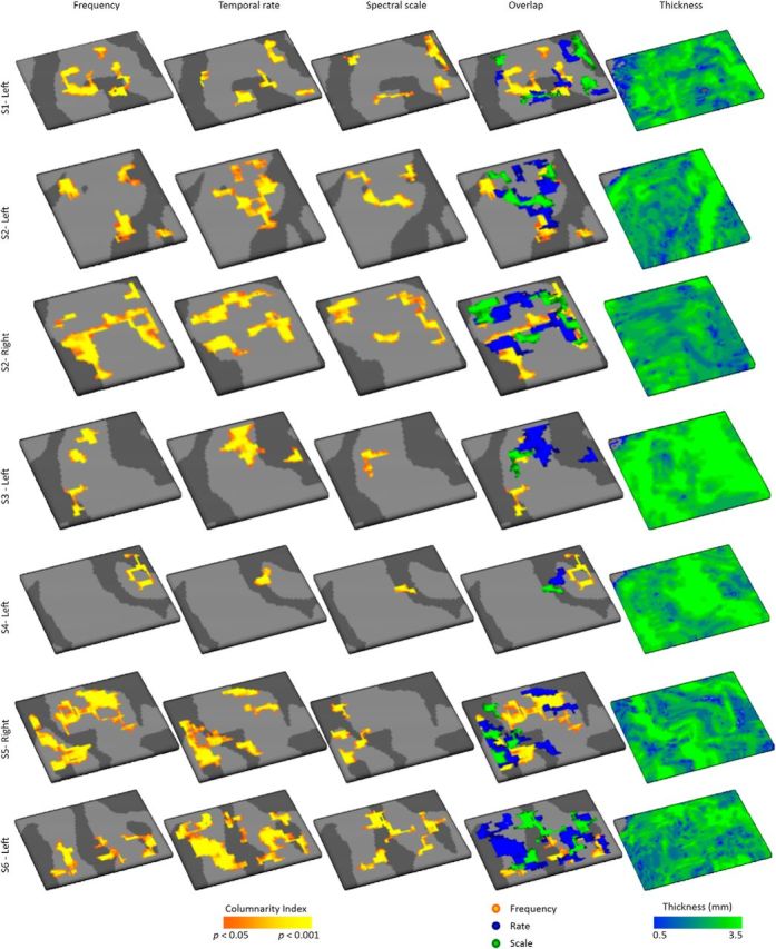
Columnarity across feature maps for all hemispheres. Significantly columnar regions for maps of preferred frequency (tonotopy), temporal modulation rate, and spectral modulation scale are shown in orange/yellow (statistics based on permutation testing). Fourth column represents the overlap of regions with a significant columnarity index across feature maps. Right-most column represents thickness of the grid is shown.

Figure 6.

Stability of columnar regions across cross-validations. For each hemisphere and feature, the stability of columnar regions is displayed as the frequency with which each gridpoint was significantly columnar across the 4 cross-validations of the dataset.

Both methods of analyzing the stability of feature preference throughout cortical depth, either as the columnarity index (i.e., the ratio of map gradients; Fig. 4C) (De Martino et al., 2015a) or as the correlation between maps at deep and superficial cortical depth (Deep-Sup; Fig. 7) (Nasr et al., 2016; Tootell and Nasr, 2017) showed that cortical depth-dependent stability was lowest for neural population tuning to spectral modulation scale and similar for maps of frequency and temporal modulation rate preference. We statistically tested differences in the columnarity index across feature maps on the results shown in Figure 4C. A two-way repeated-measures ANOVA with factors Feature [frequency, rate, scale] × Region [PAC, non-PAC] showed that the percentage of columnar cortex was different across features (main effect of Feature; F_(2,16) = 6.98, p = 0.007) and between primary and nonprimary cortex (main effect of Region; F_(2,16) = 10.94, p = 0.011; no significant interaction; Fig. 4C). Across regions, subsequent paired t tests showed that the temporal rate maps had a significantly higher columnarity index than the spectral scale maps (t₍₈₎ = 4.15, p (corrected) = 0.005). A larger part of the frequency maps than the spectral scale maps was columnar, but this difference did not reach statistical significance after correction for multiple comparisons (t₍₈₎ = 2.52; p (corrected) = 0.054 for the frequency-scale comparison). No difference was observed between the temporal modulation rate and frequency maps (t₍₈₎ = 1.44; p (corrected) = 0.282 for the rate-frequency comparison).

Figure 7.

Correlation of feature preference along and orthogonal to the cortical sheet. Graphs represent the correlation between feature preference in deep cortical depths across various distances, and between deep and superficial cortical depth (i.e., “Deep-Sup”) in (A) PAC and (B) non-PAC. Higher and lower correlation across cortical distance reflects more and less smooth feature maps, respectively. Higher correlation between deep and superficial cortical depth indicates a more columnar organization.

As a result of the definition of the columnarity index (i.e., the ratio between changes along vs orthogonal to the cortical sheet), this index is susceptible to differences in cortical thickness. To counteract this bias, the permutation-based threshold was computed per gridpoint. Accordingly, we observed a negative correlation between permutation-based threshold and thickness (mean correlation across hemispheres: r = −0.078, r = −0.066, and r = −0.058, for frequency, temporal rate, and spectral scale, respectively). Thus, the threshold for significance was higher in regions where the cortex was thinner. Use of this gridpoint-specific threshold ensured that no significant difference in cortical thickness between columnar and noncolumnar regions was observed (mean thickness: 2.68 mm and 2.80 mm inside and outside columnar regions, respectively; paired t test: t = 1.503, p = 0.171).

The columnarity index will be high for regions that have relatively stable radial feature preference and for regions with a rapid change in feature preference in the tangential direction. To discriminate between these two scenarios, we next evaluated the smoothness of the feature maps in the tangential direction as the correlation of feature preference in deep cortical depths across cortical distance (Fig. 7). Higher and lower correlation across cortical distance reflects more and less smooth feature maps, respectively. Across feature maps, the correlation dropped rapidly with increasing cortical distance. This drop was marginally faster for the spectral modulation scale maps than for the other two topographic maps but was overall very similar across features and between PAC and non-PAC.

Finally, we also evaluated the correlation between deep and superficial layers for maps of frequency, temporal modulation rate, and spectral modulation scale. In PAC, this correlation equals 0.10, 0.14, and 0.04; and in non-PAC, it equals 0.14, 0.11, and 0.04 for the three feature maps. In comparison, cortical regions at the same depth at a distance of 2.68 mm, which is equal to the average thickness of the grid, showed an average correlation of 0.07 and 0.08 in PAC and non-PAC, respectively. These results corroborate the finding of parts of auditory cortex with stable tuning to frequency and temporal modulation rate throughout cortical depth. However, the overall relatively low correlation between feature tuning on deep and superficial cortical depths also highlights the fact that substantial regions of both PAC and non-PAC are not columnar.

Discussion

We combined fMRI encoding with ultra-high field functional measurements of the auditory cortex to evaluate the cortical depth-dependent stability (implemented through the computation of a columnarity index) of tuning to frequency, temporal modulation rate, and spectral modulation scale. Results suggest relatively stable tuning to temporal modulation rates and frequency, but a transformation in spectral modulation tuning throughout the depth of HG. Across sound features, tuning of a larger cortical region in PAC than non-PAC was stable across cortical depth.

The term “columnar” has been used with different meaning across previous investigations (Horton and Adams, 2005; Rakic, 2008). Recent fMRI studies explored the presence of columnar preferences in two ways. First, Nasr et al. (2016) related the correlation in neural tuning throughout depth to the correlation in deep gray matter at a cortical distance for which a difference in neural tuning was expected (see also Tootell and Nasr, 2017). While this approach works well for regions where the spatial regularity of a columnar pattern is known (i.e., in cases of hypothesis testing in a predefined ROI), it is not feasible to set a statistical threshold in cases where information about the spatial regularity of underlying maps is absent or an ROI is not available. The second approach defined the columnarity index as the ratio between the tuning gradients along and orthogonal to the cortical sheet, and assigned significance based on permutation testing (De Martino et al., 2015a). The advantage of this approach is that it does not require a priori knowledge about the spatial regularity of underlying maps (i.e., it is suitable for an exploratory analysis), but it has the disadvantage that the interpretation of results can be ambiguous. That is, a higher columnarity index will be observed for regions with a more stable feature preference throughout depth, but also for regions with more rapid changes in feature preference along the cortical sheet. A lower columnarity index will be observed for regions with a variable preference throughout the cortical depth, but also for regions where feature preference varies little along the cortical sheet (i.e., smooth maps). Here we ran statistical analyses on results from the second approach but used results of the first approach (i.e., the decrease in correlation with increased distance between gridpoints) to evaluate map smoothness. Results across methods were in agreement; and because the spectral modulation scale maps were less smooth (i.e., feature preference changed more rapidly along the cortical sheet) than maps of temporal modulation rate and frequency, this ruled out map smoothness as an explanation for the lower columnarity index observed in spectral modulation maps.

The higher variability in spectral modulation tuning throughout cortical depth compared with temporal modulation rate and frequency tuning is in accordance with previous electrophysiological results. That is, based on invasive recordings in cat PAC, it was observed that tuning to temporal modulations was strongly columnar, whereas tuning to spectral modulations displayed more variability within a column (columnar in ∼70% vs 30% of the penetrations for temporal and spectral modulation tuning, respectively) (Atencio and Schreiner, 2010). Spectral modulation tuning was observed to change quite drastically with depth position, and this depth-dependent change was different across cortical locations. This was suggested to reflect a diversity in columnar processing, as opposed to the presence of a common information flow through the vertical canonical microcircuit (Atencio and Schreiner, 2010). While the cortical depth-dependent variation in spectral modulation scale tuning observed in the current study could reflect a similar change in spectral modulation tuning as observed in the auditory cortex of the cat, the resolution at which we map tuning to spectral modulations (5 logarithmically spaced bins ranging from 0.25 to 4 cycles/octave) limits the suitability of our current analysis to answer questions regarding the exact shape and complexity of spectral modulation tuning. In future studies, comparing the performance of encoding models that vary in shape restrictions of resulting voxel receptive fields (e.g., testing independent vs joint feature tuning) (Santoro et al., 2014) may be used to test the presence (or absence) of regular changes in spectral modulation processing throughout the auditory cortical canonical microcircuit.

For each of the mapped features, we observed columnar regions and regions with variable preference throughout cortical depth. The observation of noncolumnar regions in maps of temporal and spectral modulation preference in PAC is in accordance with results from electrophysiology (Atencio and Schreiner, 2010), yet results from invasive electrophysiology studies reported columnar frequency tuning throughout PAC (Abeles and Goldstein, 1970; Merzenich et al., 1975). As fMRI has better coverage than invasive electrophysiology, previous invasive studies could have missed depth-dependent variations in frequency preference. Alternatively, our results could represent a difference across species. Finally, our results could reflect the restrictive nature of the columnarity index used here. That is, our operationalization of columnar cortical regions may have caused us to underestimate the columnarity in auditory cortex. That is, we define columnar cortical regions as those regions where the acoustic feature preference variation along the cortical sheet (tangentially) divided by the acoustic feature preference variation through depth (radially) is significantly greater than expected by chance. This implies that significantly columnar regions may only be found in regions where the tangential map varies in at least one direction along the cortical surface. If the tangential map does not vary in a specific location, that location will not be indicated as being columnar, even if it is tuned to the exact same value in deep, middle, and superficial depths (such locations would be interpreted as “columnar” following the definition used in electrophysiology studies). Especially for smooth maps (e.g., tonotopy), our columnarity results represent a strict and lower boundary estimate of the columnar part of auditory cortex.

The observation that columnar regions did not overlap across feature maps suggests that the sound transformation throughout the auditory cortical microcircuit may vary from location to location. That is, our results support a coding strategy consisting of spatially confined modules in which part of the neuronal tuning properties is kept constant throughout cortical depth, whereas tuning to other features is systematically varied. Such a coding strategy would be in accordance with tuning to other acoustic features in auditory cortex (e.g., binaural interactions, intensity threshold, and range of spectral integration), which also display a modular organization of neural tuning preference along the auditory cortical sheet (Read et al., 2001, 2002; Linden and Schreiner, 2003).

We observed that columnar feature processing was more extensive in PAC than non-PAC as defined on the basis of myelin-related anatomical images. So far, electrophysiological investigations of columnar processing did not extend beyond primary regions in auditory cortex (Schreiner et al., 2011), and our result highlights the advantage in coverage that fMRI has compared with other methods of neuroscientific investigation. As a cautionary note, it is important to point out that our results could be due to the noninvasive PAC definition that we used. The PAC cannot be defined based on gyral/sulcal landmarks as the location of PAC varies with macroanatomy (Hackett et al., 2001; Da Costa et al., 2011). Neither can it be based on tonotopic maps (Rauschecker and Tian, 2004); and, as a result, a variety of noninvasive functional and anatomical measures beyond tonotopy have been proposed to identify the PAC (Wessinger et al., 2001; Barton et al., 2012; Moerel et al., 2012). Here we used myelin-related contrast maps to noninvasively identify PAC (Glasser and Van Essen, 2011; Dick et al., 2012; De Martino et al., 2015b). However, as myelination varies gradually throughout the STP, the applied threshold to segregate PAC from non-PAC is necessarily arbitrary and the PAC definition necessarily suboptimal. We considered the half of the grid with the highest myelin-related contrast as the PAC. Throughout hemispheres, we localized PAC to the posteromedial part of HG, consistent with results from cytoarchitecture (Galaburda and Sanides, 1980; Rivier and Clarke, 1997; Hackett et al., 2001; Morosan et al., 2001). It is certainly possible that our definition of PAC did not cover the complete PAC, but it is likely that the region we refer to as PAC is indeed fully situated within the primary auditory cortex.

In conclusion, using high field high-resolution fMRI, we have shown a relatively stable (columnar) tuning to frequency and temporal modulations, but more variable spectral modulation tuning throughout the cortical depth of both primary and nonprimary human auditory cortex. Furthermore, the observed lack of overlap of columnar regions across acoustic features suggests a modular coding strategy throughout cortical depth, with stable tuning to some features and variable tuning to others. Recent work has shown that neural tuning to acoustic features in the auditory cortex is extremely flexible and can rapidly adapt to changing task demands (Fritz et al., 2003). Moreover, as attention-induced changes were shown to be cortical depth-dependent (O'Connell et al., 2014; De Martino et al., 2015a), it is feasible that the columnar organizational principles of auditory cortex will only fully emerge when subjects are engaged in meaningful tasks. It is therefore imperative that future studies explore columnar processing during changes in context, attention, and task performance.

References

- Abeles M, Goldstein MH Jr (1970) Functional architecture in cat primary auditory cortex: columnar organization and organization according to depth. J Neurophysiol 33:172–187. 10.1152/jn.1970.33.1.172 [DOI] [PubMed] [Google Scholar]
- Atencio CA, Schreiner CE (2010) Laminar diversity of dynamic sound processing in cat primary auditory cortex. J Neurophysiol 103:192–205. 10.1152/jn.00624.2009 [DOI] [PMC free article] [PubMed] [Google Scholar]
- Atencio CA, Sharpee TO, Schreiner CE (2009) Hierarchical computation in the canonical auditory cortical circuit. Proc Natl Acad Sci U S A 106:21894–21899. 10.1073/pnas.0908383106 [DOI] [PMC free article] [PubMed] [Google Scholar]
- Barton B, Venezia JH, Saberi K, Hickok G, Brewer AA (2012) Orthogonal acoustic dimensions define auditory field maps in human cortex. Proc Natl Acad Sci U S A 109:20738–20743. 10.1073/pnas.1213381109 [DOI] [PMC free article] [PubMed] [Google Scholar]
- Brugge JF, Merzenich MM (1973) Responses of neurons in auditory cortex of the macaque monkey to monaural and binaural stimulation. J Neurophysiol 36:1138–1158. 10.1152/jn.1973.36.6.1138 [DOI] [PubMed] [Google Scholar]
- Cheng K, Waggoner RA, Tanaka K (2001) Human ocular dominance columns as revealed by high-field functional magnetic resonance imaging. Neuron 32:359–374. 10.1016/S0896-6273(01)00477-9 [DOI] [PubMed] [Google Scholar]
- Chi T, Gao Y, Guyton MC, Ru P, Shamma S (1999) Spectro-temporal modulation transfer functions and speech intelligibility. J Acoust Soc Am 106:2719–2732. 10.1121/1.428100 [DOI] [PubMed] [Google Scholar]
- Chi T, Ru P, Shamma SA (2005) Multiresolution spectrotemporal analysis of complex sounds. J Acoust Soc Am 118:887–906. 10.1121/1.1945807 [DOI] [PubMed] [Google Scholar]
- Clarey JC, Barone P, Imig TJ (1994) Functional organization of sound direction and sound pressure level in primary auditory cortex of the cat. J Neurophysiol 72:2383–2405. 10.1152/jn.1994.72.5.2383 [DOI] [PubMed] [Google Scholar]
- Da Costa S, van der Zwaag W, Marques JP, Frackowiak RS, Clarke S, Saenz M (2011) Human primary auditory cortex follows the shape of Heschl's gyrus. J Neurosci 31:14067–14075. 10.1523/JNEUROSCI.2000-11.2011 [DOI] [PMC free article] [PubMed] [Google Scholar]
- De Martino F, Zimmermann J, Muckli L, Ugurbil K, Yacoub E, Goebel R (2013) Cortical depth dependent functional responses in humans at 7T: improved specificity with 3D GRASE. PLoS One 8:e60514. 10.1371/journal.pone.0060514 [DOI] [PMC free article] [PubMed] [Google Scholar]
- De Martino F, Moerel M, Ugurbil K, Goebel R, Yacoub E, Formisano E (2015a) Frequency preference and attention effects across cortical depths in the human primary auditory cortex. Proc Natl Acad Sci U S A 112:16036–16041. 10.1073/pnas.1507552112 [DOI] [PMC free article] [PubMed] [Google Scholar]
- De Martino F, Moerel M, Xu J, van de Moortele PF, Ugurbil K, Goebel R, Yacoub E, Formisano E (2015b) High-resolution mapping of myeloarchitecture in vivo: localization of auditory areas in the human brain. Cereb Cortex 25:3394–3405. 10.1093/cercor/bhu150 [DOI] [PMC free article] [PubMed] [Google Scholar]
- Dick F, Tierney AT, Lutti A, Josephs O, Sereno MI, Weiskopf N (2012) In vivo functional and myeloarchitectonic mapping of human primary auditory areas. J Neurosci 32:16095–16105. 10.1523/JNEUROSCI.1712-12.2012 [DOI] [PMC free article] [PubMed] [Google Scholar]
- Elliott TM, Theunissen FE (2009) The modulation transfer function for speech intelligibility. PLoS Comput Biol 5:e1000302. 10.1371/journal.pcbi.1000302 [DOI] [PMC free article] [PubMed] [Google Scholar]
- Feinberg DA, Harel N, Ramanna S, Ugurbil K, Yacoub E (2008) Sub-millimeter single-shot 3D GRASE with inner volume selection for T2-weighted fMRI applications at 7 Tesla. In: 16th Annual Meeting of the International Society for Magnetic Resonance in Medicine, Toronto. [Google Scholar]
- Formisano E, Kim DS, Di Salle F, van de Moortele PF, Ugurbil K, Goebel R (2003) Mirror-symmetric tonotopic maps in human primary auditory cortex. Neuron 40:859–869. 10.1016/S0896-6273(03)00669-X [DOI] [PubMed] [Google Scholar]
- Fritz J, Shamma S, Elhilali M, Klein D (2003) Rapid task-related plasticity of spectrotemporal receptive fields in primary auditory cortex. Nat Neurosci 6:1216–1223. 10.1038/nn1141 [DOI] [PubMed] [Google Scholar]
- Galaburda A, Sanides F (1980) Cytoarchitectonic organization of the human auditory cortex. J Comp Neurol 190:597–610. 10.1002/cne.901900312 [DOI] [PubMed] [Google Scholar]
- Glasser MF, Van Essen DC (2011) Mapping human cortical areas in vivo based on myelin content as revealed by t1- and t2-weighted MRI. J Neurosci 31:11597–11616. 10.1523/JNEUROSCI.2180-11.2011 [DOI] [PMC free article] [PubMed] [Google Scholar]
- Goebel R, Esposito F, Formisano E (2006) Analysis of functional image analysis contest (FIAC) data with brainvoyager QX: from single-subject to cortically aligned group general linear model analysis and self-organizing group independent component analysis. Hum Brain Mapp 27:392–401. 10.1002/hbm.20249 [DOI] [PMC free article] [PubMed] [Google Scholar]
- Hackett TA, Preuss TM, Kaas JH (2001) Architectonic identification of the core region in auditory cortex of macaques, chimpanzees, and humans. J Comp Neurol 441:197–222. 10.1002/cne.1407 [DOI] [PubMed] [Google Scholar]
- Herdener M, Esposito F, Scheffler K, Schneider P, Logothetis NK, Uludag K, Kayser C (2013) Spatial representations of temporal and spectral sound cues in human auditory cortex. Cortex 49:2822–2833. 10.1016/j.cortex.2013.04.003 [DOI] [PubMed] [Google Scholar]
- Hoerl AE, Kennard RW (1970a) Ridge regression: biased estimation for nonorthogonal problems. Technometrics 12:55–67. 10.1080/00401706.1970.10488634 [DOI] [Google Scholar]
- Hoerl AE, Kennard RW (1970b) Ridge regression: applications to nonorthogonal problems. Technometrics 12:69–82. 10.1080/00401706.1970.10488635 [DOI] [Google Scholar]
- Horton JC, Adams DL (2005) The cortical column: a structure without a function. Philos Trans R Soc Lond B Biol Sci 360:837–862. 10.1098/rstb.2005.1623 [DOI] [PMC free article] [PubMed] [Google Scholar]
- Jones EG. (2000) Microcolumns in the cerebral cortex. Proc Natl Acad Sci U S A 97:5019–5021. 10.1073/pnas.97.10.5019 [DOI] [PMC free article] [PubMed] [Google Scholar]
- Jones SE, Buchbinder BR, Aharon I (2000) Three-dimensional mapping of cortical thickness using Laplace's equation. Hum Brain Mapp 11:12–32. 10.1002/1097-0193(200009)11:1%3C12::AID-HBM20%3E3.0.CO;2-K [DOI] [PMC free article] [PubMed] [Google Scholar]
- Joris PX, Schreiner CE, Rees A (2004) Neural processing of amplitude-modulated sounds. Physiol Rev 84:541–577. 10.1152/physrev.00029.2003 [DOI] [PubMed] [Google Scholar]
- Kay KN, David SV, Prenger RJ, Hansen KA, Gallant JL (2008a) Modeling low-frequency fluctuation and hemodynamic response timecourse in event-related fMRI. Hum Brain Mapp 29:142–156. 10.1002/hbm.20379 [DOI] [PMC free article] [PubMed] [Google Scholar]
- Kay KN, Naselaris T, Prenger RJ, Gallant JL (2008b) Identifying natural images from human brain activity. Nature 452:352–355. 10.1038/nature06713 [DOI] [PMC free article] [PubMed] [Google Scholar]
- Kay KN, Rokem A, Winawer J, Dougherty RF, Wandell BA (2013) GLMdenoise: a fast, automated technique for denoising task-based fMRI data. Front Neurosci 7:247. 10.3389/fnins.2013.00247 [DOI] [PMC free article] [PubMed] [Google Scholar]
- Kemper VG, De Martino F, Emmerling TC, Yacoub E, Goebel R (2018) High resolution data analysis strategies for mesoscale human functional MRI at 7 and 9.4T. Neuroimage 164:48–58. 10.1016/j.neuroimage.2017.03.058 [DOI] [PMC free article] [PubMed] [Google Scholar]
- Langers DR, van Dijk P (2012) Mapping the tonotopic organization in human auditory cortex with minimally salient acoustic stimulation. Cereb Cortex 22:2024–2038. 10.1093/cercor/bhr282 [DOI] [PMC free article] [PubMed] [Google Scholar]
- Linden JF, Schreiner CE (2003) Columnar transformations in auditory cortex? A comparison to visual and somatosensory cortices. Cereb Cortex 13:83–89. 10.1093/cercor/13.1.83 [DOI] [PubMed] [Google Scholar]
- Mendelson JR, Schreiner CE, Sutter ML, Grasse KL (1993) Functional topography of cat primary auditory cortex: responses to frequency-modulated sweeps. Exp Brain Res 94:65–87. [DOI] [PubMed] [Google Scholar]
- Menon RS, Ogawa S, Strupp JP, Uğgurbil K (1997) Ocular dominance in human V1 demonstrated by functional magnetic resonance imaging. J Neurophysiol 77:2780–2787. 10.1152/jn.1997.77.5.2780 [DOI] [PubMed] [Google Scholar]
- Merzenich MM, Knight PL, Roth GL (1975) Representation of cochlea within primary auditory cortex in the cat. J Neurophysiol 38:231–249. 10.1152/jn.1975.38.2.231 [DOI] [PubMed] [Google Scholar]
- Moerel M, De Martino F, Formisano E (2012) Processing of natural sounds in human auditory cortex: tonotopy, spectral tuning, and relation to voice sensitivity. J Neurosci 32:14205–14216. 10.1523/JNEUROSCI.1388-12.2012 [DOI] [PMC free article] [PubMed] [Google Scholar]
- Moerel M, De Martino F, Santoro R, Ugurbil K, Goebel R, Yacoub E, Formisano E (2013) Processing of natural sounds: characterization of multipeak spectral tuning in human auditory cortex. J Neurosci 33:11888–11898. 10.1523/JNEUROSCI.5306-12.2013 [DOI] [PMC free article] [PubMed] [Google Scholar]
- Moerel M, De Martino F, Uğgurbil K, Yacoub E, Formisano E (2015) Processing of frequency and location in human subcortical auditory structures. Sci Rep 5:17048. 10.1038/srep17048 [DOI] [PMC free article] [PubMed] [Google Scholar]
- Moerel M, De Martino F, Kemper VG, Schmitter S, Vu AT, Uğgurbil K, Formisano E, Yacoub E (2018) Sensitivity and specificity considerations for fMRI encoding, decoding, and mapping of auditory cortex at ultra-high field. Neuroimage 164:18–31. 10.1016/j.neuroimage.2017.03.063 [DOI] [PMC free article] [PubMed] [Google Scholar]
- Morosan P, Rademacher J, Schleicher A, Amunts K, Schormann T, Zilles K (2001) Human primary auditory cortex: cytoarchitectonic subdivisions and mapping into a spatial reference system. Neuroimage 13:684–701. 10.1006/nimg.2000.0715 [DOI] [PubMed] [Google Scholar]
- Mountcastle VB. (1997) The columnar organization of the neocortex. Brain 120:701–722. 10.1093/brain/120.4.701 [DOI] [PubMed] [Google Scholar]
- Nasr S, Polimeni JR, Tootell RB (2016) Interdigitated color- and disparity-selective columns within human visual cortical areas V2 and V3. J Neurosci 36:1841–1857. 10.1523/JNEUROSCI.3518-15.2016 [DOI] [PMC free article] [PubMed] [Google Scholar]
- Nieuwenhuys R. (2013) The myeloarchitectonic studies on the human cerebral cortex of the Vogt-Vogt school, and their significance for the interpretation of functional neuroimaging data. Brain Struct Funct 218:303–352. 10.1007/s00429-012-0460-z [DOI] [PubMed] [Google Scholar]
- O'Connell MN, Barczak A, Schroeder CE, Lakatos P (2014) Layer specific sharpening of frequency tuning by selective attention in primary auditory cortex. J Neurosci 34:16496–16508. 10.1523/JNEUROSCI.2055-14.2014 [DOI] [PMC free article] [PubMed] [Google Scholar]
- Oshio K, Feinberg DA (1991) GRASE (Gradient- and spin-echo) imaging: a novel fast MRI technique. Magn Reson Med 20:344–349. 10.1002/mrm.1910200219 [DOI] [PubMed] [Google Scholar]
- Phillips DP, Irvine DR (1981) Responses of single neurons in physiologically defined primary auditory cortex (AI) of the cat: frequency tuning and responses to intensity. J Neurophysiol 45:48–58. 10.1152/jn.1981.45.1.48 [DOI] [PubMed] [Google Scholar]
- Phillips DP, Irvine DR (1983) Some features of binaural input to single neurons in physiologically defined area AI of cat cerebral cortex. J Neurophysiol 49:383–395. 10.1152/jn.1983.49.2.383 [DOI] [PubMed] [Google Scholar]
- Rakic P. (2008) Confusing cortical columns. Proc Natl Acad Sci U S A 105:12099–12100. 10.1073/pnas.0807271105 [DOI] [PMC free article] [PubMed] [Google Scholar]
- Rauschecker JP, Tian B (2004) Processing of band-passed noise in the lateral auditory belt cortex of the rhesus monkey. J Neurophysiol 91:2578–2589. 10.1152/jn.00834.2003 [DOI] [PubMed] [Google Scholar]
- Read HL, Winer JA, Schreiner CE (2001) Modular organization of intrinsic connections associated with spectral tuning in cat auditory cortex. Proc Natl Acad Sci U S A 98:8042–8047. 10.1073/pnas.131591898 [DOI] [PMC free article] [PubMed] [Google Scholar]
- Read HL, Winer JA, Schreiner CE (2002) Functional architecture of auditory cortex. Curr Opin Neurobiol 12:433–440. 10.1016/S0959-4388(02)00342-2 [DOI] [PubMed] [Google Scholar]
- Rivier F, Clarke S (1997) Cytochrome oxidase, acetylcholinesterase, and NADPH-diaphorase staining in human supratemporal and insular cortex: evidence for multiple auditory areas. Neuroimage 6:288–304. 10.1006/nimg.1997.0304 [DOI] [PubMed] [Google Scholar]
- Rodríguez FA, Read HL, Escabí MA (2010) Spectral and temporal modulation tradeoff in the inferior colliculus. J Neurophysiol 103:887–903. 10.1152/jn.00813.2009 [DOI] [PMC free article] [PubMed] [Google Scholar]
- Santoro R, Moerel M, De Martino F, Goebel R, Ugurbil K, Yacoub E, Formisano E (2014) Encoding of natural sounds at multiple spectral and temporal resolutions in the human auditory cortex. PLoS Comput Biol 10:e1003412. 10.1371/journal.pcbi.1003412 [DOI] [PMC free article] [PubMed] [Google Scholar]
- Schönwiesner M, Zatorre RJ (2009) Spectro-temporal modulation transfer function of single voxels in the human auditory cortex measured with high-resolution fMRI. Proc Natl Acad Sci U S A 106:14611–14616. 10.1073/pnas.0907682106 [DOI] [PMC free article] [PubMed] [Google Scholar]
- Schreiner CE, Froemke RC, Atencio CA (2011) Spectral processing in auditory cortex. In: The auditory cortex (Winer JA, Schreiner CE, eds), pp 275–308. New York, NY: Springer. [Google Scholar]
- Sugimoto S, Sakurada M, Horikawa J, Taniguchi I (1997) The columnar and layer-specific response properties of neurons in the primary auditory cortex of mongolian gerbils. Hear Res 112:175–185. 10.1016/S0378-5955(97)00119-6 [DOI] [PubMed] [Google Scholar]
- Tootell RB, Nasr S (2017) Columnar segregation of magnocellular and parvocellular streams in human extrastriate cortex. J Neurosci 37:8014–8032. 10.1523/JNEUROSCI.0690-17.2017 [DOI] [PMC free article] [PubMed] [Google Scholar]
- Van de Moortele PF, Auerbach EJ, Olman C, Yacoub E, Uğgurbil K, Moeller S (2009) T1-weighted brain images at 7 tesla unbiased for proton density, T2* contrast and RF coil receive B1 sensitivity with simultaneous vessel visualization. Neuroimage 46:432–446. 10.1016/j.neuroimage.2009.02.009 [DOI] [PMC free article] [PubMed] [Google Scholar]
- Waehnert MD, Dinse J, Weiss M, Streicher MN, Waehnert P, Geyer S, Turner R, Bazin PL (2014) Anatomically motivated modeling of cortical laminae. Neuroimage 93:210–220. 10.1016/j.neuroimage.2013.03.078 [DOI] [PubMed] [Google Scholar]
- Wessinger CM, VanMeter J, Tian B, Van Lare J, Pekar J, Rauschecker JP (2001) Hierarchical organization of the human auditory cortex revealed by functional magnetic resonance imaging. J Cogn Neurosci 13:1–7. [DOI] [PubMed] [Google Scholar]
- Yacoub E, Shmuel A, Logothetis N, Uğgurbil K (2007) Robust detection of ocular dominance columns in humans using Hahn spin echo BOLD functional MRI at 7 tesla. Neuroimage 37:1161–1177. 10.1016/j.neuroimage.2007.05.020 [DOI] [PMC free article] [PubMed] [Google Scholar]
- Yacoub E, Harel N, Ugurbil K (2008) High-field fMRI unveils orientation columns in humans. Proc Natl Acad Sci U S A 105:10607–10612. 10.1073/pnas.0804110105 [DOI] [PMC free article] [PubMed] [Google Scholar]
- Zimmermann J, Goebel R, De Martino F, van de Moortele PF, Feinberg D, Adriany G, Chaimow D, Shmuel A, Uğgurbil K, Yacoub E (2011) Mapping the organization of axis of motion selective features in human area MT using high-field fMRI. PLoS One 6:e28716. 10.1371/journal.pone.0028716 [DOI] [PMC free article] [PubMed] [Google Scholar]