Parametric and Nonparametric Tests in Spine Research: Why Do They Matter?

I wouldn’t have seen it if I didn’t believe it.

—Attributed to Yogi Berra

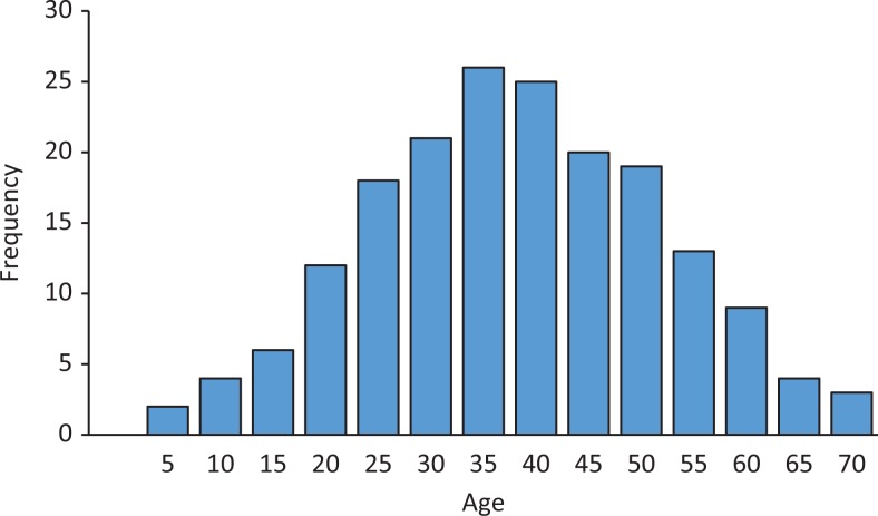
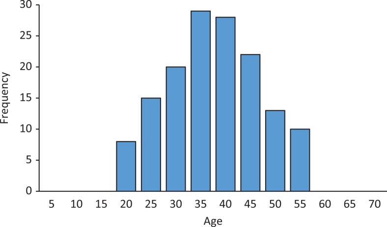
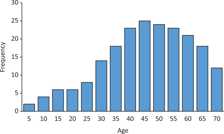
Let us begin this article with the obvious—in the process of data analysis, always look at the data first. By that we mean investigators look first at the numerical and graphical summaries of the data. Checking out the data first provides an overview of the overall project, gives a clearer understanding of the variables and their values, and shows how the values are distributed. How the data is distributed (data distribution) is characterized by its center, its spread, and the shape of the data. The center refers to the middle of the value distribution, along with an estimate of the value typical of the data. Spread simply refers to how far “spread out” the data points are. Are the values close to the center or are they widely spread out, and are there significant outliers? The shape of a distribution is described by its number of peaks and by presence (or absence) of symmetry. Figure 1 contains the distribution of age for a hypothetical example. The center of distribution is around 38 years. Figure 2 has less spread than the distribution in Figure 1 though the center is about the same. Both distributions are symmetrical with a single peak. Figure 3, on the other hand, is not symmetrical but skewed to the right. When a distribution is similar to Figure 1, we refer to that distribution as a normal distribution. Many statistical tests assume that the data is normally distributed. But what if they are not?

Figure 1.

Age distribution with a mean of 38 years, spread out from age 5 to age 70, and symmetrical on both sides of the mean.

Figure 2.

Mean age similar to Figure 1 but with a tighter distribution.

Figure 3.

Age distribution not symmetrical but skewed to the right.

Parametric Versus Nonparametric Tests

Parametric and nonparametric tests are broad classifications of statistical testing procedures. They are perhaps more easily grasped by illustration than by definition. Remember that when we conduct a research project, our goal is to discover some “truth” about a population and the effect of an intervention on that population. Since it is not possible to collect data from all individuals in a population at large, we collect data from a sample or subset of individuals from the population. We refer to means, standard deviations, and proportions as “parameters” when we are talking about a population in general. We then estimate those “parameters” from our sample. When we calculate sample estimates, we refer to these quantities as “statistics.” A statistic estimates a parameter. Parametric statistical procedures assume that the sample distribution is about the same shape (ie, normally distributed) and has the same parameters (ie, means and standard deviations) as the general population distribution. Nonparametric statistical procedures make no such assumptions about the shape or parameters of the population distribution.

When to Use Qualitative Data

Qualitative data, also known as “categorical data,” is defined by a category and grouped by characteristics and are then given a name rather than by a measured numeric expression. Qualitative or categorical data count the number of individuals or observations in each category, such a history of opiate abuse, American Spinal Injury Association (ASIA) grade, or category of type of surgery. The ability to delineate the effect of an intervention within subgroups of a population rests on appropriate qualitative grouping within a population.

Categorical data is classified as 2 types, nominal or ordinal. “Nominal” variables are groups described by name rather than by number and exist without order or rank associating the groups. Examples of “nominal” variables are gender, cause of injury, category of surgery, payor status (eg, public insured, private insured, self-pay). “Nominal” variables can also be identified as presence or absence of a condition or state measured as yes/no. When the variable has only 2 possible categories it is referred to as binary or dichotomous. Examples of dichotomous nominal variables are history of intravenous drug use, yes/no; history of opiate abuse, yes/no; and epidural abscess, yes/no.

“Ordinal” data is similar to nominal data by categorical grouping; however, grouping has natural order or rank. Examples of “ordinal” variables are groupings of progressive quantities of morphine equivalents per day, pathology severity such as Meyerding grade (I, II, III, IV, V), and of measures of impairment such as ASIA grade (A, B, C, D, E). It is important to note, while “ordinal” categories reflect groupings of natural order such as ASIA grade, the difference between each category is not necessarily uniform. For example, impairment is progressively greater starting with ASIA Grade E (normal) and finishing with ASIA Grade A (no sensory or motor function); however, the difference between ASIA Grades A and B may not be the same as between ASIA Grades B and C, particularly with prediction of future function.¹

Table 1 illustrates the use of qualitative data when comparing coordination of surgical intervention.

Table 1.

Illustration of How to Display Categorical Data Comparing Coordination of Intervention.

	Overlapping Surgery (n = 1505)	Nonoverlapping Surgery (n = 1800)
Lumbar fusion less than 3 levels, n (%)	310 (21)	325 (18)
Lumbar fusion greater than 3 levels, n (%)	150 (10)	178 (10)

When to Use Quantitative Data Not Normally Distributed

Quantitative or numeric data is associated with numeric values that have usually been obtained by measurements rather than categories or groups. “Quantitative” or “numeric” data is categorized as either discrete or continuous. “Quantitative” data is discrete when they cannot be more precise, that is, often a count involves whole integers such as the patient’s number of lumbar vertebra or number of previous surgeries. “Continuous” data is data that can be further divided and comprise values spanning the breadth of possible measurements such as age, height, weight, or magnitude of scoliosis primary curve. When graphed, discreet or continuous data values will display as grouped around a bell-shaped curve (normally distributed) or not grouped around a bell-shaped curve (not normally distributed). Quantitative data not normally distributed is used in study of a variable resulting in variation across a continuum, not aggregated uniformly around the mean. When this is the case, identification of such is critical in the decision process of test selection for identification of differences.

Which Test to Use

The decision on which statistical analysis test to select, aimed to result in the greatest power, rests initially on the assessment of whether a data set reflects approximately normal distribution or reflects approximately not normal distribution. Parametric tests (which utilize mean as measurement of central tendency) should be employed for analysis of normal distribution, whereas nonparametric tests (which utilize median as measurement of central tendency) should be employed for analysis of data not normally distributed (see Table 2). Once a decision is made selecting a parametric or nonparametric test, individual test selection rests on the characteristics of group and variable design, that is, number of groups, number of tests, and so on.

Table 2.

Illustration of Parametric and Nonparametric Analysis Decision Tree.

	2 Independent Groups	2 Dependent Groups	>2 Independent Groups	>2 Dependent Groups
Parametric	N > 30	Sample sizes equal	No minimum n	No minimum n
				Sample sizes equal
	Independent t test	Dependent t test	One-way ANOVA	Repeated-measures ANOVA
Nonparametric	N ≥ 8	N ≥ 5	No minimum n	No minimum n
	Mann-Whitney	Wilcoxon	Kruskal-Wallis	Friedman’s ANOVA

Abbreviation: ANOVA, analysis of variance.

What Happens If the Wrong Test Is Used?

With correct assumptions (eg, normal distribution), parametric methods will have more power to detect differences than nonparametric methods. However, using a parametric test when assumptions are violated results in a “lack of power.” That is, when analyzing data not normally distributed with parametric tests, the investigator is more likely to fail to detect a difference in the source population when one truly exists (Type II error).

Summary

• Parametric and nonparametric are 2 broad classifications of statistical procedures.

• Parametric tests are based on assumptions about the distribution of the underlying population from which the sample was taken. The most common parametric assumption is that data is approximately normally distributed.

• Nonparametric tests do not rely on assumptions about the shape or parameters of the underlying population distribution.

• Use nonparametric tests for categorical data or continuous data that is not normally distributed.

• The decision on which statistical test to select for analysis can be aided by using a decision tree such as the one given in the text above.

• Rethink how you approach evaluating a study in the future. Consider looking at the data first and reviewing its characteristics, the shape and the type of data gathered. And then see what the authors chose to do with their data. Assessing research in this manner will assist in determining the validity of the investigators’ methods and subsequent results reporting.