Classification of suspicious lesions on prostate multiparametric MRI using machine learning

Abstract.

We present a radiomics-based approach developed for the SPIE-AAPM-NCI PROSTATEx challenge. The task was to classify clinically significant prostate cancer in multiparametric (mp) MRI. Data consisted of a “training dataset” (330 suspected lesions from 204 patients) and a “test dataset” (208 lesions/140 patients). All studies included T2-weighted (T2-W), proton density-weighted, dynamic contrast enhanced, and diffusion-weighted imaging. Analysis of the images was performed using the MIM imaging platform (MIM Software, Cleveland, Ohio). Prostate and peripheral zone contours were manually outlined on the T2-W images. A workflow for rigid fusion of the aforementioned images to T2-W was created in MIM. The suspicious lesion was outlined using the high b-value image. Intensity and texture features were extracted on four imaging modalities and characterized using nine histogram descriptors: 10%, 25%, 50%, 75%, 90%, mean, standard deviation, kurtosis, and skewness (216 features). Three classification methods were used: classification and regression trees (CART), random forests, and adaptive least absolute shrinkage and selection operator (LASSO). In the held out by the organizers test dataset, the areas under the curve (AUCs) were: 0.82 (random forests), 0.76 (CART), and 0.76 (adaptive LASSO). AUC of 0.82 was the fourth-highest score of 71 entries (32 teams) and the highest for feature-based methods.

1. Introduction

Prostate cancer is the most common cancer in American men.¹ Clinical decisions, related to the need for prostate biopsy, which areas to biopsy, and regions that require attention in focally directed therapy, are multifactorial and complex. The use of multiparametric MRI (mpMRI) for detecting prostate cancer is rapidly evolving because of its growing availability and ability to combine functional [perfusion via dynamic contrast-enhanced (DCE-MRI) and diffusion via diffusion-weighted imaging (DWI)], and anatomical information [T2-weighted (T2-W) MRI]. The combined information in the multiple mpMRI sequences results in high sensitivity and specificity for distinguishing intraprostatic cancer of higher grade [Gleason score (GS) 7 or above].^2,3 To standardize the evaluation and reporting of prostate mpMRI, an expert panel of the European Society of Urogenital Radiology published in 2012 the prostate imaging reporting and data system (PI-RADS) for prostate cancer detection⁴ (current version PI-RADSv.2).⁵

Unlike PI-RADS, which largely depends on subjective assessment of mpMRI, computer-aided diagnosis (CAD) techniques for quantitative mpMRI analysis have also been developed for prostate cancer detection and diagnosis.^6–12 The core components in CAD systems for prostate cancer, as summarized by Liu et al.¹³ and Lemaitre et al.,¹⁴ include preprocessing of the images, segmentation of the prostate, image registration between MRI modalities, feature extraction, and voxel classification. The CAD efforts can be divided into two categories based on the main objectives for the analysis: (i) detection/segmentation of the suspicious lesion and/or (ii) assessment of the aggressiveness of prostate cancer.¹⁵ In 2016, the International Society for Optics and Photonics (SPIE), along with the support of the American Association of Physicists in Medicine (AAPM) and the National Cancer Institute (NCI), conducted a “grand challenge” on quantitative image analysis methods for the diagnostic classification of clinically significant prostate lesions.¹⁶ As opposed to the detection task, the location of the suspicious lesion in the SPIE-AAPM-NCI PROSTATEx challenge was provided and the goal was to decide if the lesion is related to clinically significant cancer ($\mathrm{GS}\ge 7$) or benign and/or low risk ($\mathrm{GS}=6$). The PROSTATEx challenge task was different from determining whether a lesion is cancerous or not,^7,9,17,18 or discriminating between GS $(3+4)=7$ and GS $(4+3)=7$.^19–21 However, the general approach for these feature-based algorithms is to compute a set of quantitative imaging features from the mpMRI data and develop a supervised classifier using the computed features from the training cases and their associated “ground-truth” labels. The developed classifier is then used to classify new cases (test dataset).

The increased applications of prostate mpMRI for clinical decision making, and the plethora of the associated imaging sequences and quantifiable features, bring forth the following questions: What are the optimal ways to analyze mpMRI data for the prostate; do all MR sequences contribute to the accuracy of the MRI interpretation; which of the imaging features have importance for the final classification?

In this paper, we present our approach for analysis of the PROSTATEx challenge data to assess the aggressiveness of the suspicious lesions.¹⁶ A collection of retrospective set of prostate MR studies was provided to the challenge participants. The data were separated in training and test datasets. The lesions in the training dataset were labeled with “TRUE” and “FALSE” for the presence of significant cancer. The assignment of the lesions in the test dataset was held back by the challenge organizers. The goal was to develop a model, based on the training dataset and using this model to classify the lesions in the test dataset. The selection of the prediction models was based on the area under the ROC curve (AUC). The predicted scores (0 to 1, 0 = benign, 1 = significant cancer) for each lesion in the test dataset were obtained using the prediction models. The predicted scores were sent to the challenge organizers and the models evaluated by AUC. The AUC results for the test dataset were communicated back to the challenge participants. The PROSTATEx challenge provided us with a unique opportunity to compare our algorithms with those of others from academia, industry, and government. We evaluated all sequences of mpMRI and investigated the importance of the imaging features to the final classification model.

2. Materials and Methods

2.1. MRI Data Description

We analyzed data from the SPIE-AAPM-NCI PROSTATEx challenge.¹⁶ The dataset represented a collection of a retrospective set of prostate mpMRI studies.¹¹ All studies included T2-W, proton density-weighted (PD-W) imaging, DCE-MRI, and DWI.²² The following description of the dataset was provided by the Challenge’s organizers: “The images were acquired on two different types of Siemens 3T MR scanners, the MAGNETOM Trio, and Skyra. T2-weighted images were acquired using a turbo spin echo sequence and had a resolution of around 0.5 mm in plane and a slice thickness of 3.6 mm. The DCE time series was acquired using a three-dimensional (3-D) turbo flash-gradient echo sequence with a resolution of around 1.5 mm in-plane, a slice thickness of 4 mm, and a temporal resolution of 3.5 s. The proton density weighted image was acquired prior to the DCE time series using the same sequence with different echo and repetition times and a different flip angle. $K^{\text{trans}}$, the volume transfer coefficient that measures capillary permeability, computed from the DCE²³ was provided in MetaImage medical format (mhd). Finally, the DWI series were acquired with a single-shot echo planar imaging sequence with a resolution of 2-mm in-plane and 3.6-mm slice thickness and with diffusion-encoding gradients in three directions. Three b-values were acquired (50, 400, and 800), and subsequently, the apparent diffusion coefficient (ADC) map was calculated by the scanner software. All images were acquired without an endorectal coil.”

The data, provided by the Challenge consisted of a training dataset of 330 suspected lesions from 204 patients and a test dataset of 208 suspected lesions from 140 patients. The approximate location of the centroid of each lesion for both datasets was provided in DICOM coordinates. The lesions were also labeled as belonging to peripheral zone (PZ), transition zone (TZ), anterior stroma (AS), and seminal vesicles (SV). The lesion distribution in the training/test dataset was: PZ: 191/113; TZ: 82/59; AS: 55/34; and SV: 2/2. The lesions in the training dataset were labeled with “TRUE” and “FALSE” for presence of significant cancer. The cancer status of the lesions in the test dataset was held back by the challenge organizers.

2.2. Image Analysis

Analysis of the images in both training and test datasets was performed using the MIM imaging platform (MIM Software, Cleveland, Ohio). The DICOM files in each dataset were loaded in MIM. The high b-value image (BVAL) was provided in a separate DICOM. $K^{\text{trans}}$ images were converted from mhd/zraw formats to DICOM. Prostate contours and PZ were manually outlined on the T2-W images. A workflow for rigid fusion was created in MIM. The spatial coregistrations used the following protocol: (i) PD-W images were rigidly aligned to T2-W and the resulting registration matrix was used to align the $K^{\text{trans}}$ map and (ii) ADC images were rigidly aligned to the T2-W and the registration matrix was used to align the BVAL. The centroid of the lesion was localized in MIM and the lesion was then outlined manually by imaging experts (RS, JCF) with more than 25 years combined expertise in prostate cancer. The lesions were crosschecked by the two imaging experts and reviewed by clinicians (SP, AP) with extensive expertise in genitourinary malignancies. Predominantly, the BVAL series were used for lesion contouring with the ADC acting as a secondary for verification. The lesion contours were then confirmed on the T2-W and $K^{\text{trans}}$ images and adjusted if needed. For each patient in the training dataset, lesions were numbered within a patient and labeled as C_Z, where C = T (true) or F (false) and Z = P (PZ) or T (TZ). Examples of four lesions are shown in Fig. 1. The lesion centroid, as provided by the challenge’s organizers, is marked with a red circle on the four analyzed sequences: T2-W, ADC, BVAL, and $K^{\text{trans}}$. For the purposes of our analysis, we did not differentiate the small number of AS and SV as distinct from the TZ, and thus they were included as part of the TZ contour.

Fig. 1.

Examples of images from the analyzed dataset. The following sequences from the multiparametric (mp)MRI were analyzed: T2-weighted MRI (T2-W), ADC, high B-value (BVAL), and $K^{\text{trans}}$. The prostate and PZ volumes were manually contoured on T2-W. Four lesions, marked with True and False in the PZ and TZ, are illustrated. The red circle marks the centroid of the lesion. Note that the “true” lesions are characterized by hypointensity on T2-W and ADC and high signal on BVAL and $K^{\text{trans}}$. The hypointensity on T2-W and high $K^{\text{trans}}$ is less specific on the “false” lesions.

2.3. Quantitative Imaging Features

The broad classes of radiomics features can be generally divided into four categories.¹⁵ The first category summarizes features descriptive of the volume size, shape, etc. The second, third, and fourth categories can be described as first-, second- and higher-order statistical outputs. First-order statistic features are related to the intensity histogram of a given volume: mean, median, standard deviation, minimum, maximum, quartiles, kurtosis, skewness, etc. The second-order statistics are related to texture analysis features, also known as Haralick texture descriptors.²⁴ Finally, the higher-order methods extract patterns using kernel functional transformation.

In our analysis, we focused on radiomics features from the first three categories. First, the prostate and lesion’s volumes were recorded. Using a Java-based plugin, the lesions’ intensities on the four image modalities (T2-W, ADC, BVAL, and $K^{\text{trans}}$) were characterized using nine histogram descriptors: 10%, 25%, 50%, 75%, 90%, mean, standard deviation, kurtosis, and skewness.

Five texture features (energy, entropy, correlation, homogeneity, and contrast) were extracted from T2-W, ADC, BVAL, and $K^{\text{trans}}$ using Haralick descriptors. The features were calculated using the gray-level co-occurrence matrices (GLCM) for each voxel underlying the contoured regions in the image. Voxel-wise texture measures were computed in 3-D by sliding a window of size $5\times 5\times 5$ across the image region enclosing the tumor volume. First, image intensities were rescaled within 0 to 256 range using the entire image. The GLCM was then computed in 3-D using 128 bins in a $5\times 5\times 5$ patch centered at each voxel.²⁰ The texture values for the whole tumor were then summarized using the voxel-wise textures. The nine histogram descriptors described above were calculated for each texture feature. The texture features were computed using C++ and the publically available Insight ToolKit software libraries for imaging (Fig. 2).

Fig. 2.

Texture features in lesion contour on T2-weighted (T2-W) MRI and ADC maps.

In summary, 216 quantitative imaging variables were analyzed: four modalities (T2-W, ADC, BVAL, and $K^{\text{trans}}$) × six features [first-order: intensity (int) and second-order: energy (ene), entropy (ent), correlation (cor), homogeneity (hom), and contrast (con)] × nine descriptors [10%, 25%, 50%, 75%, 90%, mean, standard deviation (SD), kurtosis (kurt), and skewness (skew)]. Here and in the rest of the text, the imaging variables names are constructed by concatenating modality, feature (abbreviated), and descriptor (abbreviated). For instance, ADC_int_50% refers to the 50% of the ADC intensity.

2.4. Classification Analysis

As imaging data are highly correlated and high dimensional, we considered three widely used techniques in variable selection: classification and regression trees (CART),²⁵ random forests,²⁶ and adaptive least absolute shrinkage and selection operator (LASSO).²⁷ The CART method is a tree-based method that utilizes a recursive search algorithm for a binary split to partition the data satisfying minimization of a splitting criterion. Three measures are widely used for a stopping criterion for splitting: misclassification rate, Gini index, and cross entropy. CART can detect interactions among variables, as well as nonmonotonic relations in predicting the outcome, and it can handle missing values.^25,28 The result of the CART is easy to interpret as it produces one tree with subjects classified into clearly defined subsets from partition of the variables analyzed. For the CART, we performed apparent validation, which used the same dataset for model building and model performance evaluation. Gini splitting method was used with the complexity of Gini splitting method that was used with the complexity parameter (minimum improvement in the model needed at each node) = 0.01, maximum tree depth = 3, and minimum bucket (number of observations in a terminal node) = 4. However, one big disadvantage of the CART is its instability, which means that a small change in the dataset might cause a hugely different result (tree structure).²⁸ Random forests were proposed as natural extension of the CART to overcome the above instability problem in the CART. Although CART generates only one tree, the random forests method grows a large number of trees (usually hundreds) to build a forest. In the random forests, we can estimate the relative importance of each variable, which includes continuous, categorical, and ordinal variable types. In the random forests, variable selection was conducted based on variable importance calculated from out-of-bag errors (errOOB) along with multiple bootstrapped datasets. In this study, we considered 2000 repetitions. We also considered one of the shrinkage methods, the adaptive LASSO. The shrinkage methods work very well in correlated high-dimensional data. The conventional LASSO is known to tend to select many unimportant variables.²⁷ The adaptive LASSO shows better performance in obtaining consistent variable selection. Important variables of the adaptive LASSO approach were selected based on importance scores calculated by the bootstrap ranking procedure along with 10-fold cross validation. We set the number of repetitions in the bootstrap to 200.

As we have a large number of variables for the prediction, to avoid overfitting we conducted variable selection in the training dataset using the three methods mentioned. CART automatically provided sets of important variables for prediction. We ran random forests to obtain variable importance scores and choose a subset of variables with mean decrease Gini $\ge 1$ to build prediction models. In addition, the bootstrap ranking scores were used in the adaptive LASSO methods to select a subset of variables. In the bootstrap ranking procedure, we obtained a LASSO estimate matrix representing variable importance ranking and intersected aggregate results to obtain robust variable selection. Variables with the highest variable importance scores were identified as a set of informative variables. The sample size of bootstrap dataset was set to equal the sample size of the training dataset. The tuning parameter for LASSO was selected using the 10-fold cross-validation. Then, the selected variables from CART, random forests, and LASSO were used to derive predictive models using logistic regression. Two separate models, one for classification of PZ lesions and another for the TZ lesions, were built by each of the three approaches and used to obtain the predicted cancer outcome scores for the training set. The AUC for each method in the training set was reported as a performance measure. We also reported 95% confidence interval for AUC in the training set using bootstrap approach (1000 repeats). These models were also used to predict the scores (0 to 1, 0 = benign, 1 = significant cancer) for each lesion in the test dataset. Analysis was performed using corresponding R packages (R Foundation for Statistical Computing).

3. Results

The results of the variable selection in the training dataset by the three methods are shown in Table 1, separately for PZ and TZ. In addition to the 216 quantitative imaging variables, the tumor relative volume was added to the variables during variable selection. Tumor relative volume was obtained using ratio of lesion volume and prostate volume. We tested the significance of the tumor relative volume using univariate logistic regression, and it was highly significant ($p<0.0001$) for both PZ and TZ. In total, there were 22 and 21 imaging variables selected for PZ and TZ, respectively. Interestingly, the contribution of the different modalities to the variables for PZ and TZ were strikingly different: about two-thirds of PZ variables were related to DWI data: ADC and BVAL; 5/22 (22%) to T2-W; and only two variables were related to $K^{\text{trans}}$. In contrast, $K^{\text{trans}}$ played more prominent role in TZ (7/21, 33%). Similarly, the composition of the radiomics features between the two zones was also quite different: $>50\%$ of the features in the PZ were intensity-related, whereas the texture variables comprised 86% from the TZ variables. Interestingly, the commonality in the "important variables" between the two zones was that the descriptors predominantly were associated with measures for heterogeneity, such as standard deviation, kurtosis and skewness: 13/22 and 19/21 for PZ and TZ, respectively.

Table 1.

Training set–variable selection by three methods using the training dataset.

	CART	Random forest plus logistic	Adaptive Lasso plus logistic
Peripheral zone	Tumor relative volume	Tumor relative volume	Tumor relative volume
	BVAL_con_90%	ADC_int_10%	T2-W_ent_75%
	ADC_int_50%	ADC_int_25%	ADC_hom_Skew
	T2-W_ene_25%	BVAL_con_90%	ADC_hom_Kurt
	T2-W_ent_Kurt	BVAL_int_90%	ADC_int_Kurt
	T2-W_int_Kurt	BVAL_int_SD	BVAL_ene_Skew
	ADC_hom_SD	$K^{\text{trans}}$_int_50%	$K^{\text{trans}}$_con_Skew
			BVAL_int_SD
			BVAL_int_Kurt
			T2-W_int_Skew
			BVAL_int_Skew
	Se = 0.73; Sp = 0.993	Se = 0.784; Sp = 0.748	Se = 0.919; Sp = 0.867
	PPV = 0.964; NPV = 0.931	PPV = 0.46; NPV = 0.927	PPV = 0.654; NPV = 0.975
	AUC = 0.907 (0.837, 0.965)a	AUC = 0.878 (0.823, 0.944)a	AUC = 0.944 (0.911, 0.990)a
Transition zone	Tumor relative volume	Tumor relative volume	Tumor relative volume
	$K^{\text{trans}}$_con_50%	BVAL_con_SD	BVAL_int_SD
	BVAL_ent_SD	$K^{\text{trans}}$_con_SD	T2-W_ene_SD
	$K^{\text{trans}}$_ene_Skew	T2-W_hom_SD	$K^{\text{trans}}$_ene_Kurt
	$K^{\text{trans}}$_int_SD		T2-W_ent_90%
			$K^{\text{trans}}$_ene_Skew
			$K^{\text{trans}}$_con_Skew
			ADC_con_Skew
			T2-W_ent_Skew
			T2-W_ene_Skew
			BVAL_con_Skew
			BVAL_ene_Skew
			ADC_ene_Skew
			ADC_hom_Skew
			BVAL_int_Skew
	Se = 0.975; Sp = 0.882;	Se = 0.925; Sp = 0.782;	Se = 0.875; Sp = 0.909;
	PPV = 0.75; NPV = 0.99	PPV = 0.607; NPV = 0.966	PPV = 0.778; NPV = 0.952
	AUC = 0.935 (0.90, 0.969)a	AUC = 0.907 (0.858, 0.957)a	AUC = 0.947 (0.933, 1)a

Note: Abbreviations: CART, classification and regression trees; LASSO, least absolute shrinkage and selection operator; Se, sensitivity; Sp, specificity; PPV, positive predictive value; NPV, negative predictive value; AUC, area under the curve.

^a95% confidence interval via bootstrap.

Figure 3 shows corresponding AUCs in the training dataset. Based on AUC, the best performance was by the adaptive LASSO method in both PZ and TZ, respectively. The bootstrap 95% CIs for AUC were shown in Table 1. In addition, we evaluated AUC for the model containing only tumor relative volume. With 200 bootstrap datasets, mean AUCs and corresponding 95% confidence intervals were 0.539 (0.464, 0.624) for PZ and 0.537 (0.471, 0.617) for TZ, respectively.

Fig. 3.

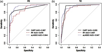
ROC curves and AUCs in the training dataset by three classification methods in (a) PZ and (b) TZ. Abbreviations: CART, classification and regression trees; RF, random forest; and LASSO, least absolute shrinkage and selection operator.

The PROSTATEx challenge organizers informed us that in the test dataset, the AUCs of our proposed three methods were as follows: 0.82 (random forests), 0.76 (CART), and 0.76 (adaptive LASSO).

Although the nature of our analysis is high dimensional and multivariate models were used for prediction, we investigated the univariable association of the individual imaging features in the training dataset with the lesion label (T/F). The goal of this analysis was to discern patterns in correlations of the individual features and image modalities. We calculated the regression coefficient of each imaging variable (i.e., logarithm of odds ratio) obtained from univariate logistic regression. These coefficients are represented graphically as heat maps on Fig. 4. The top panel contains the analysis for the PZ lesions, and the bottom for TZ. In each row, 54 coefficients are displayed: nine descriptors [10%, 25%, median (50%), mean, 75%, 90%, SD, kurt, and skew] for each of the six features. There are four rows for each modality: T2-W, ADC, BVAL, and $K^{\text{trans}}$. For instance, the intensities of BVAL are positively correlated with significant cancer, i.e., the higher the BVAL, the higher is the probability for significant cancer. In concordance of the results from the variable selection above, the last three columns (histogram descriptors standard deviation, kurtosis and skewness) in each of the boxes contain the highest number of significant correlations.

Fig. 4.

Univariable analysis for association of imaging variables with lesions aggressiveness in the training dataset: the regression coefficients from univariate logistic regression are displayed as a heat-map in shades of blue (negative associations) to red (positive associations). Each imaging feature (intensity, contrast, correlation, energy, entropy, and homogeneity) is characterized by nine attributes (10%, 25%, med, avr, 75%, 90%, sd, kurt, and skew) displayed in the $x$ axis. The imaging variables in each row are associated with particular sequence (T2-W, ADC, BVAL, and $K^{\text{trans}}$). The imaging variables for the PZ are displayed in the top panel and for the transition zone–bottom panel.

4. Discussion

Automated prostate cancer classification has been investigated by different research groups. The underlying schema of the algorithm consists of feature extraction and classification. In this paper, we present a radiomics-based approach developed for the SPIE-AAPM-NCI PROSTATEx challenge. The goal of our participation was to compare the performance of our model in the test dataset with other groups. The result obtained from the random forests classification, AUC of 0.82, was the fourth-highest score of 71 entries (from 32 teams) and the highest score for feature-based approach in the PROSTATEx Challenge. Our results were comparable with the reported in the literature AUC values achieved by the experienced human reader: 0.79 and 0.83 for PI-RADS v1 and PI-RADS v2, respectively.²⁹

As radiomic features are sensitive to variations in matrix size, resolution, signal-to-noise ratio, and pulse sequence parameters including TR/TE,^30–35 differences between training and test data may affect the performance of the model. However, the random forest model for the training data resulted in AUC of $\sim 0.88$. The performance of this model was reported by the organizers as AUC = 0.82 in the held-out test dataset, indicating that the proposed model generalizes well on the test data.

There are numerous ways to compute image textures. In Wibmer et al.,¹⁹ texture features were computed over the whole 3-D volume defined by the lesion contour. In Nketiah et al.,²¹ the computation is done in 64 bins and in 4 directions. Our approach for texture extraction is identical to Fern et al.²⁰ However, we use nine histogram descriptors for each feature rather than only the mean. Although many of the histogram descriptors may be correlated with one another, we do not know a priori which ones may be clinically useful radiomic features; therefore, we felt it prudent to include as many as seemed reasonable and to let the statistical analysis weed out the unnecessary ones by determining which are correlated to clinically significant cancer and which are redundant. In addition, in this paper, texture analysis was applied also to $K^{\text{trans}}$. Even in this highly variable approach, a common finding is that T2-W and ADC entropy (mean) are correlated with GS. Although this variable does not appear in the variable selection list (Table 1), mean/median of entropy on T2-W and ADC shows high correlations in our univariable analysis (Fig. 4). It is possible that these associations are masked by entropy’s standard deviation, kurtosis, and skewness in our analysis, for example, variables that were not investigated previously.

Tumor relative volume was selected as an important variable by all models. The radiomics features, however, unlike the ones used in the radiology lexicon (size, shape, and location), are agnostic.³⁶ Our analysis indicated that the presence of lesion heterogeneity (multiple physiologically distinct regions within the tumor), demonstrated by overrepresentation of standard deviation, kurtosis, and skewness in the model-selected variables, is a major discriminating factor for the prostatic lesions. This is consistent to our current understanding of cancer cells microenvironmental distribution that consists of heterogeneous cell populations in contrast to nonmalignant ones.³⁶

Some participants in the PROSTATEx challenge utilized deep learning approaches such as convolutional neural networks (CNN).^37,38 The advent of deep CNN techniques has led to great success in image classification.^39,40 It should be noted that our radiomics-based approach also outperformed some CNN applications.⁴¹ We suggest that this robustness may be due in part to the expertise in contouring the suspicious lesions as well as in the precision of the MIM image fusion between the different modalities. Although there is large inter-expert variability in delineating prostate cancer, we assume that in the case that the lesion centroid is provided, these variations are reduced by at least assuring that all lesions are detected and boundaries are drawn in the correct vicinity. However, a proper study for determining these variations should be carried out.

This study has several limitations. First, the TZ, AS, and SV lesions were combined in one category (TZ). The reason is that combining the three types of lesions (TZ, AS, and SC) resulted in a larger dataset to build a predictive multivariable model (from 82 to 139 lesions). The rationale for combining these lesions was that both TZ and AS are composed of mostly stromal tissues. In contrast to PZ, TZ, and AS have similar imaging characteristics: they appear darker than the PZ on T2 and ADC and brighter on DCE-MRI. The contrast on T2 and ADC reflects the different amounts of macromolecular and free water presence. The PZ is composed of highly glandular-ductal tissues, resulting in brighter signal on T2 and ADC in PZ. TZ and AS are better vascularized than PZ and the contrast agent enters at a higher rate relative to the healthy prostatic glands or ducts.⁴² Another limitation of the study is that additional preprocessing steps could have been carried out to mitigate the differences in acquisition parameters between the datasets. Image intensities were not normalized prior to characterization of the intensity feature, whereas intensities were scaled between 0 and 256 prior to texture features extraction. There is a variety of algorithms for image intensity normalization such as image standardization,⁴³ N4-bias field correction,⁴⁴ and histogram equalization.⁴⁵ Linearly interpolating the data to a set resolution ($1\times 1\times 1\mathrm{mm}$, for example) would lessen the spatial resolution differences between the datasets.

In a future study, we will investigate a separate predictive model for AS when we have a sufficient number of lesions in this location. Future plans also involve investigation into the relative importance of the different mpMRI sequences. The data in the PROSTATEx Challenge will serve as an invaluable resource for comparing preprocessing methods for removing the acquisition variations between the datasets. Once the test dataset is unmasked by the PROSTATEx organizers, we will carry analysis to determine a minimal set of significant radiomics variable that will yield similar AUCs.

Biographies

Deukwoo Kwon is a statistician who has been actively involved in imaging/radiomics research at the University of Miami. He has expertise in regression models, classification, generalized linear models, and Bayesian methods.

Isildinha M. Reis is a research professor at the Department of Public Health Sciences at the University of Miami and in the Biostatistics and Bioinformatics Shared Resource (BBSR) at the Sylvester Comprehensive Cancer Center. One of her research interest is the statistical modeling of binary and time to event patient outcomes.

Adrian L. Breto is a recent graduate of the Department of Computer Engineering at the University of Miami’s College of Engineering. Currently, he is a graduate student in the same department. His research interests involve design, programming, and implementation of advanced software for quantitative image analysis of mpMRI.

Yohann Tschudi has a doctoral degree in physics. During his postdoctoral training, his work has focused on multimodality detection/diagnosis/prognosis of prostate cancer and the performance evaluation of radiomics methods.

Nicole Gautney is an undergraduate at Florida International University, majoring in biology. Her research interests include medical imaging.

Olmo Zavala-Romero has a doctoral degree in Scientific Computing. His work is focused on applications of machine learning to medical imaging. His research interests are in deep learning and computer vision.

Christopher Lopez has a doctoral degree in chemistry with emphasis on NMR. During his postdoctoral training, his work has focused on multivariable analysis of imaging.

John C. Ford is an assistant professor in the Department of Radiation Oncology at University of Miami. A therapeutic medical physicist, he has a strong research background in MRI. His research interests are in utilization of MRI in image-guided adaptive radiotherapy and quantitative imaging for prediction of treatment response.

Sanoj Punnen is an assistant professor at the Department of Urology at the University of Miami. His research interests are centered on the management of patients with prostate cancer, involving mpMRI as a tool for risk assessment.

Alan Pollack is a professor and chair of the Department of Radiation Oncology at the University of Miami. His research interests are centered on the management of prostate cancer patients. A particular interest of his is to apply quantitative imaging and genomic (radiogenomic) methods, to identify prostate habitats that determine outcome, as applied to selecting patients for active surveillance and selecting at risk volumes for radiotherapy targeting.

Radka Stoyanova is a professor and director of Imaging and Biomarkers at the Department of Radiation Oncology at the University of Miami. Her research interests mainly involve the investigation of CAD and radiomics methods for the assessment of risk, diagnosis, prognosis, and response to therapy of prostate cancer on mpMRI.

Disclosures

No conflicts of interest, financial or otherwise, are declared by the authors.

References

- 1.Siegel R. L., Miller K. D., Jemal A., “Cancer statistics, 2018,” CA Cancer J. Clin. 68(1), 7–30 (2018). 10.3322/caac.v68.1 [DOI] [PubMed] [Google Scholar]
- 2.Isebaert S., et al. , “Multiparametric MRI for prostate cancer localization in correlation to whole-mount histopathology,” J. Magn. Reson. Imaging 37(6), 1392–1401 (2013). 10.1002/jmri.23938 [DOI] [PubMed] [Google Scholar]
- 3.Futterer J. J., et al. , “Can clinically significant prostate cancer be detected with multiparametric magnetic resonance imaging? A systematic review of the literature,” Eur. Urol. 68(6), 1045–1053 (2015). 10.1016/j.eururo.2015.01.013 [DOI] [PubMed] [Google Scholar]
- 4.Barentsz J. O., et al. , “ESUR prostate MR guidelines 2012,” Eur. Radiol. 22(4), 746–757 (2012). 10.1007/s00330-011-2377-y [DOI] [PMC free article] [PubMed] [Google Scholar]
- 5.Mclean R. A., Sanders W. L., Stroup W. W., “A unified approach to mixed linear-models,” Am. Stat. 45(1), 54–64 (1991). 10.2307/2685241 [DOI] [Google Scholar]
- 6.Tiwari P., et al. , “Quantitative evaluation of multi-parametric MR imaging marker changes post-laser interstitial ablation therapy (LITT) for epilepsy,” Proc. SPIE 8671, 86711Y (2013). 10.1117/12.2008157 [DOI] [PMC free article] [PubMed] [Google Scholar]
- 7.Kwak J. T., et al. , “Automated prostate cancer detection using T2-weighted and high-b-value diffusion-weighted magnetic resonance imaging,” Med. Phys. 42(5), 2368–2378 (2015). 10.1118/1.4918318 [DOI] [PMC free article] [PubMed] [Google Scholar]
- 8.Turkbey B., et al. , “Multiparametric 3T prostate magnetic resonance imaging to detect cancer: histopathological correlation using prostatectomy specimens processed in customized magnetic resonance imaging based molds,” J. Urol. 186(5), 1818–1824 (2011). 10.1016/j.juro.2011.07.013 [DOI] [PMC free article] [PubMed] [Google Scholar]
- 9.Khalvati F., Wong A., Haider M. A., “Automated prostate cancer detection via comprehensive multi-parametric magnetic resonance imaging texture feature models,” BMC Med. Imaging 15, 27 (2015). 10.1186/s12880-015-0069-9 [DOI] [PMC free article] [PubMed] [Google Scholar]
- 10.Haider M. A., et al. , “Combined T2-weighted and diffusion-weighted MRI for localization of prostate cancer,” Am. J. Roentgenol. 189(2), 323–328 (2007). 10.2214/AJR.07.2211 [DOI] [PubMed] [Google Scholar]
- 11.Litjens G., et al. , “Computer-aided detection of prostate cancer in MRI,” IEEE Trans. Med. Imaging 33(5), 1083–1092 (2014). 10.1109/TMI.2014.2303821 [DOI] [PubMed] [Google Scholar]
- 12.Litjens G. J., et al. , “Quantitative identification of magnetic resonance imaging features of prostate cancer response following laser ablation and radical prostatectomy,” J. Med. Imaging (Bellingham) 1(3), 035001 (2014). 10.1117/1.JMI.1.3.035001 [DOI] [PMC free article] [PubMed] [Google Scholar]
- 13.Liu L., et al. , “Computer-aided detection of prostate cancer with MRI: technology and applications,” Acad. Radiol. 23(8), 1024–1046 (2016). 10.1016/j.acra.2016.03.010 [DOI] [PMC free article] [PubMed] [Google Scholar]
- 14.Lemaitre G., et al. , “Computer-aided detection and diagnosis for prostate cancer based on mono and multi-parametric MRI: a review,” Comput. Biol. Med. 60, 8–31 (2015). 10.1016/j.compbiomed.2015.02.009 [DOI] [PubMed] [Google Scholar]
- 15.Stoyanova R., et al. , “Prostate cancer radiomics and the promise of radiogenomics,” Transl. Cancer Res. 5(4), 432–447 (2016). 10.21037/tcr [DOI] [PMC free article] [PubMed] [Google Scholar]
- 16.Litjens G. J. S., et al. , “ProstateX challenge data,” Cancer Imaging Arch. (2017). [Google Scholar]
- 17.Litjens G. J. S., et al. , “Distinguishing prostate cancer from benign confounders via a cascaded classifier on multi-parametric MRI,” Proc. SPIE 9035, 903512 (2014). 10.1117/12.2043751 [DOI] [Google Scholar]
- 18.Litjens G. J. S., et al. , “Computer-extracted features can distinguish noncancerous confounding disease from prostatic adenocarcinoma at multiparametric MR imaging,” Radiology 278(1), 135–145 (2016). 10.1148/radiol.2015142856 [DOI] [PMC free article] [PubMed] [Google Scholar]
- 19.Wibmer A., et al. , “Haralick texture analysis of prostate MRI: utility for differentiating non-cancerous prostate from prostate cancer and differentiating prostate cancers with different Gleason scores,” Eur. Radiol. 25(10), 2840–2850 (2015). 10.1007/s00330-015-3701-8 [DOI] [PMC free article] [PubMed] [Google Scholar]
- 20.Fehr D., et al. , “Automatic classification of prostate cancer Gleason scores from multiparametric magnetic resonance images,” Proc. Natl. Acad. Sci. U. S. A. 112(46), E6265–E6273 (2015). 10.1073/pnas.1505935112 [DOI] [PMC free article] [PubMed] [Google Scholar]
- 21.Nketiah G., et al. , “T2-weighted MRI-derived textural features reflect prostate cancer aggressiveness: preliminary results,” Eur. Radiol. 27(7), 3050–3059 (2017). 10.1007/s00330-016-4663-1 [DOI] [PubMed] [Google Scholar]
- 22.Clark K., et al. , “The Cancer Imaging Archive (TCIA): maintaining and operating a public information repository,” J. Digit. Imaging 26(6), 1045–1057 (2013). 10.1007/s10278-013-9622-7 [DOI] [PMC free article] [PubMed] [Google Scholar]
- 23.Tofts P. S., “Modeling tracer kinetics in dynamic Gd-DTPA MR imaging,” J. Magn. Reson. Imaging 7(1), 91–101 (1997). 10.1002/(ISSN)1522-2586 [DOI] [PubMed] [Google Scholar]
- 24.Haralick R. M., “Statistical and structural approaches to texture,” Proc. IEEE 67(5), 786–804 (1979). 10.1109/PROC.1979.11328 [DOI] [Google Scholar]
- 25.Breiman J. H., et al. , CART: Classification and Regression Trees, Chapman & Hall/CRC, Boca Raton, Florida: (1984). [Google Scholar]
- 26.Breiman L., “Random forests,” Mach. Learn. 45(1), 5–32 (2001). 10.1023/A:1010933404324 [DOI] [Google Scholar]
- 27.Zou H., “The adaptive lasso and its oracle properties,” J. Am. Stat. Assoc. 101(476), 1418–1429 (2006). 10.1198/016214506000000735 [DOI] [Google Scholar]
- 28.Hastie T., Tibshirani R., Friedman J. H., The Elements of Statistical Learning: Data Mining, Inference, and Prediction, Springer, New York: (2009). [Google Scholar]
- 29.Kasel-Seibert M., et al. , “Assessment of PI-RADS v2 for the detection of prostate cancer,” Eur. J. Radiol. 85(4), 726–731 (2016). 10.1016/j.ejrad.2016.01.011 [DOI] [PubMed] [Google Scholar]
- 30.Herlidou-Meme S., et al. , “MRI texture analysis on texture test objects, normal brain and intracranial tumors,” Magn. Reson. Imaging 21(9), 989–993 (2003). 10.1016/S0730-725X(03)00212-1 [DOI] [PubMed] [Google Scholar]
- 31.Jirak D., Dezortova M., Hajek M., “Phantoms for texture analysis of MR images, long-term and multi-center study,” Med. Phys. 31(3), 616–622 (2004). 10.1118/1.1646231 [DOI] [PubMed] [Google Scholar]
- 32.Mayerhoefer M. E., et al. , “Effects of MRI acquisition parameter variations and protocol heterogeneity on the results of texture analysis and pattern discrimination: an application-oriented study,” Med. Phys. 36(4), 1236–1243 (2009). 10.1118/1.3081408 [DOI] [PubMed] [Google Scholar]
- 33.Savio S. J., et al. , “Effect of slice thickness on brain magnetic resonance image texture analysis,” Biomed. Eng. Online 9(9), 60 (2010). 10.1186/1475-925X-9-60 [DOI] [PMC free article] [PubMed] [Google Scholar]
- 34.Waugh S. A., “The influence of field strength and different clinical breast MRI protocols on the outcome of texture analysis using foam phantoms,” Med. Phys. 38(9), 5058–5066 (2011). 10.1118/1.3622605 [DOI] [PubMed] [Google Scholar]
- 35.Peng Y., et al. , “A study of T-2-weighted MR image texture features and diffusion-weighted MR image features for computer-aided diagnosis of prostate cancer,” in Medical Imaging 2013: Computer-Aided Diagnosis, Novak C. L., Aylward S., Eds., Vol. 8670, SPIE, Bellingham, Washington: (2013). [Google Scholar]
- 36.Gillies R. J., Kinahan P. E., Hricak H., “Radiomics: images are more than pictures, they are data,” Radiology 278(2), 563–577 (2016). 10.1148/radiol.2015151169 [DOI] [PMC free article] [PubMed] [Google Scholar]
- 37.Liu S. F., et al. , “Prostate cancer diagnosis using deep learning with 3D multiparametric MRI,” Med. Imaging Comput.-Aided Diagn. 10134, 1013428 (2017). [Google Scholar]
- 38.Seah J. C. Y., Tang J. S. N., Kitchen A., “Detection of prostate cancer on multiparametric MRI - a ProstateX challenge runner up,” Med. Imaging Comput.-Aided Diagn. 10134, 1013429 (2017). [Google Scholar]
- 39.Krizhevsky A., Sutskever I., Hinton G. E., “ImageNet classification with deep convolutional neural networks,” Commun. ACM. 60(6), 84–90 (2017). 10.1145/3098997 [DOI] [Google Scholar]
- 40.Simonyan K., Zisserman A., Criminisi A., “Immediate structured visual search for medical images,” Med. Image Comput. Comput. Assist. Interv. 14(Pt 3), 6893, 288–296 (2011). 10.1007/978-3-642-23626-6_36 [DOI] [PubMed] [Google Scholar]
- 41.Mehrtash A., et al. , “Classification of clinical significance of MRI prostate findings using 3D convolutional neural networks,” Proc. SPIE 10134, 101342A (2017). 10.1117/12.2277123 [DOI] [PMC free article] [PubMed] [Google Scholar]
- 42.Noworolski S. M., et al. , “Dynamic contrast-enhanced MRI and MR diffusion imaging to distinguish between glandular and stromal prostatic tissues,” Magn. Reson. Imaging 26(8), 1071–1080 (2008). 10.1016/j.mri.2008.01.033 [DOI] [PMC free article] [PubMed] [Google Scholar]
- 43.Nyul L. G., Udupa J. K., “On standardizing the MR image intensity scale,” Magn. Reson. Med. 42(6), 1072–1081 (1999). 10.1002/(ISSN)1522-2594 [DOI] [PubMed] [Google Scholar]
- 44.Tustison N. J., et al. , “N4ITK: improved N3 bias correction,” IEEE Trans. Med. Imaging 29(6), 1310–1320 (2010). 10.1109/TMI.2010.2046908 [DOI] [PMC free article] [PubMed] [Google Scholar]
- 45.Hum Y. C., Lai K. W., Salim M. I. M., “Multiobjectives bihistogram equalization for image contrast enhancement,” Complexity 20(2), 22–36 (2014). 10.1002/cplx.v20.2 [DOI] [Google Scholar]