Image Quality Evaluation in Clinical Research: A Case Study on Brain and Cardiac MRI Images in Multi-Center Clinical Trials

Abstract

Magnetic resonance imaging (MRI) system images are important components in the development of drugs because it can reveal the underlying pathology in diseases. Unfortunately, the processes of image acquisition, storage, transmission, processing, and analysis can influence image quality with the risk of compromising the reliability of MRI-based data. Therefore, it is necessary to monitor image quality throughout the different stages of the imaging workflow. This report describes a new approach to evaluate the quality of an MRI slice in multi-center clinical trials. The design philosophy assumes that an MRI slice, such as all natural images, possess statistical properties that can describe different levels of contrast degradation. A unique set of pixel configuration is assigned to each possible level of contrast-distorted MRI slice. Invocation of the central limit theorem results in two separate Gaussian distributions. The central limit theorem says that the mean and standard deviation of pixel configuration assigned to each possible level of contrast degradation will follow a normal distribution. The mean of each normal distribution corresponds to the mean and standard deviation of the underlying ideal image. Quality prediction processes for a test image can be summarized into four steps. The first step extracts local contrast feature image from the test image. The second step computes the mean and standard deviation of the feature image. The third step separately standardizes each normal distribution using the mean and standard deviation computed from the feature image. This gives two separate z-scores. The fourth step predicts the lightness contrast quality score and the texture contrast quality score from cumulative distribution function of the appropriate normal distribution. The proposed method was evaluated objectively on brain and cardiac MRI volume data using four different types and levels of degradation. The four types of degradation are Rician noise, circular blur, motion blur, and intensity nonuniformity also known as bias fields. Objective evaluation was validated using a proposed variation of difference of mean opinion scores. Results from performance evaluation show that the proposed method will be suitable to monitor and standardize image quality throughout the different stages of imaging workflow in large clinical trials. MATLAB implementation of the proposed objective quality evaluation method can be downloaded from (https://github.com/ezimic/Image-Quality-Evaluation).

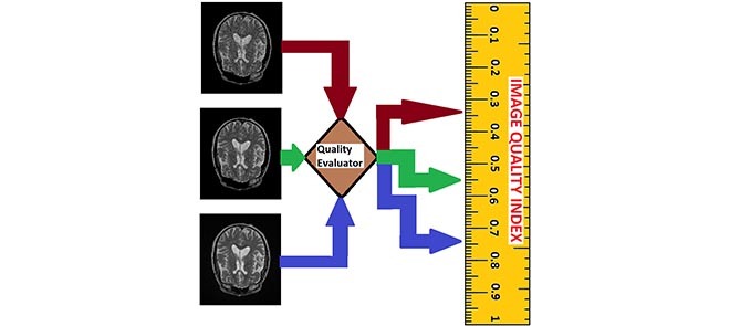
This report describes a new approach to evaluate the quality of an MRI cardiac or brain slice in multi-center clinical trials.

I. Introduction

Magnetic resonance imaging (MRI) system has several features which makes it a popular imaging modality in routine clinical practice and clinical research [1]. Patient safety is satisfied by its non-invasive and non-ionizing properties. Images acquired from MRI system can potentially discriminate the different anatomical structures with high spatial and contrast resolution [2]. This feature makes MRI system useful tool for the study of human anatomy and the diagnosis of diseases. Diagnostic information contained in MRI images are enriched by MRI three perpendicular planes display of images. Furthermore, MRI system is highly flexible. The different imaging sequences generated from a scan can be deployed for different clinical tasks.

Applications of brain MRI include monitoring disease progression in multiple sclerosis and Alzheimer’s diseases [3], [4], clinical trials of drugs for the diagnosis and treatment of multiple sclerosis and Alzheimer’s diseases [5], [6], performance evaluation of different MRI sequences in brain analysis [7], [8], comparative performance evaluation of clinical trials of different drugs for the treatment of multiple sclerosis [9], [10], study of brain atrophy [11], [12], evaluation of pediatric multiple sclerosis [13], [14], safety and efficacy of drugs for the treatment of multiple sclerosis [15], [16].

Cardiac MRI is used for the assessment of cardiac structure and function such as the characterization of myocardial tissue, blood volume and blood flow measurements [17]–[19]. Other applications include the diagnosis of cardiac amyloidosis [20], identification of regions with left ventricle hypertrophy [21]. Evaluation of pathology in congenital heart disease, cardiac masses, cardiomyopathies and valvular heart diseases [19].

A typical setup of large clinical trial consist of multiple locations across the globe. Each location is referred to as clinical trial site. Multiple clinical trial sites interact with a clinical research organization (CRO). The CRO manages the clinical trial of drugs for the sponsoring pharmaceutical organization. Three major activities are carried out at the clinical trial sites. They are enrolment of subjects, administration of the drug under trial to subjects and the acquisition of images from MRI system. Daily, several thousands of slices contained in hundreds of MRI volume data are routed from the clinical trial sites to a CRO.

The quality of a medical image can be assessed either in terms of its measurable physical properties or the medical goal of the image [22]. Measurable physical properties include visual attributes such as texture, contrast, sharpness and noise. The medical goal of the image is the task of the imaging system from which the image was acquired [23], [24]. The following characteristics and requirements in a large clinical trial justify the need for a no-reference objective quality evaluation of MRI images.

• 1)Quality Monitoring Through Stages of Imaging Workflow: The task of acquisition, storage, transmission, processing and analysis can have adverse effect on image quality. The potential of an MRI system to generate high contrast image can be reduced by improper system parameter settings. Concern for patient comfort may require trade-off between signal-to-noise ratio, image resolution and length of scan time [25]. MRI signal is sensitive to motion [26]. It is extremely difficult for a subject to maintain ideal pose during every visit for image acquisition. Patient motion and the manifestations of physiological functions such as breathing and heart beat introduces blur and artifacts during acquisition [27], [28]. The processes of storage and transmission of images can introduce blur and blocking which reduces image details and sharpness [29]. Wavelet and total variation approaches to the removal of noise, deblurring and enhancement introduce ringing artifacts and blurred edges resulting in loss of diagnostic information in the images [30]–[32].
• 2)Limitations of Subjective Quality Evaluation: Subjective evaluation by human observers is regarded as the gold standard for quality evaluation. However several factors limits its application in large clinical trials. Trained experts cannot cope with the large volume of data that are processed in clinical trials [33]. Human emotions, environmental and lighting conditions influence subjective evaluation by radiologists and trained MRI readers resulting in intra and inter expert variability [33]–[35]. Efficient processing and the management of MRI data demand real-time operation offered by objective quality evaluation. There is little tolerance for the cumbersomeness and the variability of the outcomes of subjective image quality evaluation.
• 3)Inter-Site Variations in MRI System Parameters: Cost-saving measures by the pharmaceutical companies requires that only MRI systems available at the clinical trial sites are utilized for acquisition. The consequences are variations in the quality of images from the different scanner manufacturers. It is impractical to construct a single image model to act as reference image for the evaluation of images from the different trial sites. In the real world there is no image having ideal qualities that can be regarded as a reference image. Thus no-reference method based on image quality attributes is a more practical approach to evaluate image quality [36]. Good clinical practice demands high level of integrity from clinical data. The reliability of metrics derived from MRI-based images acquired from the different clinical trials sites, to a large extent, is dependent on the re-evaluation and standardization of image quality before data analysis.
• 4)Intra-Subject Variations in Acquisition Parameters: Images of a subject acquired at different time points requires registration before analysis. There is also the possibility of scanner change at the clinical trial sites for clinical trials that span over a period of time. Intensity mismatch is common occurrence between images acquired at different time points. Processing tasks such as intensity normalization and image registration demands quality re-evaluation to assess the integrity of information contained in the images.
• 5)Conformity With Acquisition Protocols: Brain measurements derived from MRI systems are susceptible to differences in imaging sequence parameters [37]. In clinical trials the sponsoring pharmaceutical organization outline acquisition protocols which include requirements on image quality to ensure optimal utility of the images and avoid inaccurate diagnosis [38], [39]. Post-acquisition image quality evaluation at the CRO is one of key steps towards conformity with the acquisition protocols.

Signal-to-noise ratio (SNR), mean square error (MSE) and peak signal-to-noise ratio (PSNR) are the popular full-reference quality evaluation methods at the acquisition stage of MRI images. Several post-acquisition evaluation methods have been proposed. The report in [40] apply analysis of variance (ANOVA) algorithm to assess the variation of several quality measures with different levels of distortions. Mortamet et al. [39] combine the detection of artifacts and estimation of noise level to measure image quality. Recently the report in [41] propose a no-reference method which predict brain MRI quality based on five quality attributes. The attributes are lightness, contrast, sharpness, texture details and noise. The report in [42] predict image quality by casting the relationship between entropy and classical image quality attributes on Bayesian framework. Another report [43] computes image quality by using three separate geo-spatial feature vectors extracted from a test image to standardize corresponding Gaussian distributed quality models. Other recent reports assess image quality based on how subject motion during acquisition bias structural information and metrics derived from the image [44]–[48]. This report provide only a brief review of image quality evaluation. Detailed review of quality evaluation methods for medical images are available in [36] and [49]–[52].

Current quality evaluation methods for MRI images are designed using different quality evaluation models for specific stages of the imaging workflow. There is no specific quality evaluation method that can effectively evaluate the quality of an image from acquisition through the different stages of the imaging workflow. Current methods such as [39], [44], and [45] which assume that background noise voxels contain information pertinent to quality of images have several shortcomings. First, they cannot be applied to parallel imaging technique which the noise level is variable across the image field of view [53]. Second, background-based noise estimation methods are only suitable for images in which the field of view allows the MRI system to capture air-tissue boundary and generate images with background that describe the surrounding air. For this reason background-based noise estimation methods will be suitable for brain MRI images but useless for cardiac and lung MRI images with small field of view because background voxels are not available. Even for brain MRI images, the performance of these algorithms can be significantly limited by underestimation of noise level when the number of background voxels are limited or corrupted by artifacts [54], [55]. The need for a large population to extract relevant features for the construction of quality model can be regarded as a drawback for the reports in [42] and [43]. This drawbacks makes it difficult to achieve the much desired consistent quality evaluation required in good clinical practice. Thus, it can be said that current algorithms are unsuitable for large clinical trials.

This paper describes a new objective, no-reference attribute-based quality evaluation method for MRI images. It is based on the application of moments-preserving property of additive linear degradation model, labeling problem and the central limit theorem to the pixel configurations that describe each possible level of contrast degradation in an MRI slice. Labeling problem is used to classify the different levels of degradation in an image.

This paper is organized as follows. The next Section describes the materials and method used for quality assessment. Section 3 displays results of the objective and subjective performance evaluation of the proposed quality metric. Results from the experiment are discussed in Section 4. Section 5 concludes this report.

II. Materials and Methods

A. Materials

1). Sources and Description of Test Data

The test data were retrospectively acquired from different models of General Electric (GE) and Siemens 1.5 and 3T scanners that use different coils, and were obtained from four different sources. The sources of data are NeuroRx research Inc. (https://www.neurorx.com), BrainCare Oy. (http://braincare.fi/), the Alzheimer’s disease neuroimaging initiative (ADNI) (http://www.adni.loni.usc.edu) and the Department of Diagnostic Imaging of the Hospital for Sick Children in Toronto, Canada (http://www.sickkids.ca/DiagnosticImaging/index.html).

There are thirty nine brain MRI volume data. They consist of fifteen T2 weighted, ten T1 Magnetization-Prepared Rapid Gradient Echo (MPRAGE) pulse sequence and fourteen conventional T1 weighted images.

All the T2 volume data were without perceived degradation. There are five, seven and three T2 volume data from NeuroRx, ADNI and BrainCare, respectively. Each T2 volume data from NeuroRx and ADNI contain 60 slices. Each slice has dimension and 2.4 mm thickness. There are 24 slices in the T2 volume data from BrainCare, each with dimension voxels and 2.6 mm thickness. The MPRAGE pulse sequence images from ADNI were without perceived degradation. Each data has 150 slice with dimension voxels and 1.2 mm thickness. All the conventional T1 MRI volume data from NeuroRx were originally acquired with various configurations of bias fields.

2). Cardiac MRI Data

There are 16 cardiac MRI volume data from the Department of Diagnostic Imaging of the Hospital for Sick Children in Toronto, Canada. The data were acquired as short axis MRI data. The images were acquired using the Fast Imaging Employing Steady State Acquisition (FIESTA) sequence protocol. The images reveal the endocardial and epicardial structures of the ventricle. The data were among the experimental data in the report [56] which describe the framework for the analysis of short axis cardiac MRI using statistical models of shape and appearance. Each volume data contain 20 frames. The number of slices in each frame varies from 8 to 15. The dimension of each slice is along the long axis.

3). Artificial Degradation

Three different types of degradation; circular blur, motion blur and Rician noise at different levels were artificially induced on the foreground and background voxels of the test data. Circular blur was simulated by convolving a slice in a volume data with circular averaging filter of radius , voxels. The range of the radius of the circular averaging filter was scaled from level 1 to level 15 in unit step. The motion blur was induced on a slice by convolving it with a special filter which approximates the linear motion of a camera. The linear motion is described by two parameters, the linear distance in voxels and the angular distance in degree. Both parameters were scaled from 1 to 15 in unit step. Two separate and identical Gaussian noise levels were generated to simulate the real and imaginary components in the complex plane of MRI acquisition process. Rician noise was added to the data by computing the magnitude of the complex data. The noise level was scaled from 1 to 15 in unit step.

B. Problem Formulation

1). Structural and Acquisition Models of MRI

Following on the contribution in [57] we model an ideal MRI slice as statistically simple and structurally piecewise constant. A slice is regarded as a two-tissue class binary image. The two-tissue class MRI slice follows the same reasoning in [58] that regard the observed grayscale image as a blurred version of an underlying binary image. With reference to a T2 weighted MRI slice the bright voxels describe the high density of edges that describe the cortical gray matter, ventricular system and the boundaries between the different anatomical structures. The white matter and other anatomical structures are described by the dark voxels.

MRI image acquisition follows the mathematical model of a 2D linear shift-invariant imaging system [59], [60], expressed by:

where is the observed grayscale image, , the underlying ideal image, can be either space-invariant point spread function or multiplicative spatially varying factor and is random noise. The random noise is independent of the image spatial coordinates and modeled as a Gaussian distribution with mean and variance .

An MRI slice is formed on a rectangular lattice. The lattice consist of sites corresponding to the location of image voxels in Euclidean space [61]:

where are the indices of the sites. Label is the set of pixel intensity levels that can be assigned to a site [61]:

where are the indices of the labels. Image labeling problem is the assignment of a label from the set to each of the site in .

2). Ideal MRI Acquisition

In the absence of any degradation, there is no random noise, the multiplying spatial varying factor and the space-invariant point spread function are identity matrix:

Under this condition the observed MRI slice possess its full natural properties and is considered the exact replica of the underlying ideal image:

Let denote the local contrast feature LCF image derived through the use of appropriate filter to extract local information from the observed image. Under an ideal acquisition condition, based on the two-tissue class model, the LCF image is a replica of the observed image as well as a replica of the underlying ideal image;

Therefore, the first and second moments of the LCF image and the observed image are equal

3). Real MRI Acquisition

The mathematical model of image acquisition expressed in Eq. 1 indicates that all the different types of degradation which are present during real MRI acquisition process are derived from three sources; random noise, the multiplying spatial varying factor and the space-invariant point spread function. In this report we generalize invariant features proposed for blur degradation by [62] to include all the different types of degradation. Specifically, in the presence of any degradation, the first and second moments of the ideal image are preserved in the observed image:

The severity of any type of degradation is denoted by integer numbers where implies absence of degradation, that is, image acquisition under ideal condition. At each level of degradation, a unique set of label referred to as image pixel configuration [61] is assigned to each site on the grid of the observed image . With reference to 8-bit grayscale image, each image pixel configuration is a sample of size 256, obtained at random, with replacement, from the population of 256 formed by 8-bit grayscale voxels. The total number of possible degradation levels is all the possible random samples .

The mean of the LCF image extracted from the observed image at each level of degradation is a random variable . According to the central limit theorem, if the number of possible degradation levels tends to infinity and is finite, the distribution of approaches a normal distribution with mean and variance :

where is the mean of the underlying ideal image .

Using the same hypothesis, the variance of the LCF image extracted from the observed image at each level of degradation is also a random variable . The central limit theorem says that the distribution of approaches a normal distribution with mean and variance :

where is the variance of the underlying ideal image .

4). Quality Prediction

Quality prediction is based on making analogy between the Gaussian distributions expressed in Eq. 12 and Eq. 13 and the power spectral density of an image. The pixel configurations assigned to an observed image at each possible level of degradation is the equivalent of all the possible frequencies contained in the image. The power of the observed image at a specific frequency is the variance of the LCF image extracted from the observed image. The maximum possible total power in the spectrum is the area under the curve that describe each probability distribution. The total power corresponds to the maximum possible image contrast [63]. Two quality scores, lightness contrast quality score and the texture contrast quality score of the test image can be predicted from the appropriate Gaussian distribution.

Given the combined effect of all the possible distortions, the lightness contrast quality score is the magnitude of perceived visual differences of local structures within the image. It is expressed by the normal cumulative distribution function of

where the standard deviation of the LCF image extracted from the test image standardize the normal distribution to obtain , the z-score:

The texture contrast quality score is the magnitude of details that describe the local structures and the different anatomical structures within the image in the presence of either blurring process or noise degradation process. It is computed from a one-tailed probability distribution:

where is the normal cumulative distribution function given that the mean of the local contrast feature image standardize one-half of the normal distribution expressed in Eq. 12 to obtain the z-score :

There are two reasons to justify the computation of the texture contrast quality score using one-half of the normal distribution. The mean of the normal distribution can be regarded as a natural threshold which separate the influence of noise and blur degradation processes. There is increase dominance of noise and blur below and above the threshold. Above the threshold, where noise dominates, the mean of the LCF image is higher than the mean of the observed image. Below the threshold, where blur dominates, the mean of the LCF image is lower than the mean of the observed image. Both degradation processes results in loss of sharpness but in opposite direction on either side of the threshold [41].

The variances, , associated with the lightness contrast quality score and the texture contrast quality score are determined using the principle of three-signal rule [64]:

The total quality score is the weighted sum of the predicted scores for the two quality attributes

where is the first moment of the test image. The philosophy behind the assignment of weight to each quality score is based on the lightness of the image. For images with higher level of lightness higher weight is assigned to the lightness contrast quality score and lower weight to the texture contrast quality score. On the other hand, images with lower level of lightness have lower weight assigned to the lightness contrast quality score and higher weight assigned to the texture contrast quality score.

C. Objective Evaluation

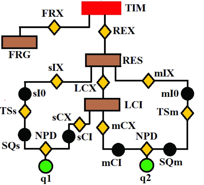
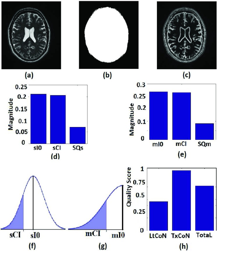
In this section we use the flow chart of Fig. 1 and the images displayed in Fig. 2 to describe the eight steps to implement our proposed no-reference quality evaluation for MRI images. The MRI slice is from a MRI volume data provided by BrainCare.

FIGURE 1.

The flow chart of our proposed no-reference quality evaluation for MRI images. The first step rescale REX the intensity level of the test image TIM to lie between 0 and 1, followed by the extraction FRX of foreground FRG. The third step computes (mIX, sIX) the first mI0 and second sI0 moments of the test image. The local contrast feature image LCI is extracted LCX in the fourth step. The fifth step computes (mCX, sCX) the first mCX and second sCX moments of the local contrast feature image. The lightness contrast quality score q1 and the texture contrast quality score q2 are computed in the sixth and seventh steps from the cumulative normal distribution function NPD of the random variables evaluated at (, ). In the last step, the total quality score is computed from the weighted sum of the lightness and contrast quality scores.

FIGURE 2.

Description of the proposed no-reference quality evaluation for MRI images. (a) The test image has its pixel intensity level rescaled to lie between 0 and 1. (b) Foreground of the test image in (a) is extracted. (c) Local contrast feature image is extracted from the test image. (d) The second moments (sI0, sCI) is computed from the test image and the local contrast feature image. The variance SQs of the normal distribution is also computed. (e) The first moments (mI0, mCI) computed from the test image and the local contrast feature image as well as the variance SQm of the normal distribution. (f) Two-tail cumulative distribution function for the computation of lightness contrast quality score. (g) One-tail cumulative distribution function for the computation of texture contrast quality score. (h) Bar chart of the lightness contrast quality score, texture contrast quality score and the total quality score.

1). Step 1 - Intensity Rescaling

The intensity level of the test image TIM shown in Fig. 2a is rescaled REX to lie between 0 and 1 so that the rescaled test image RES in Fig. 2b can be regarded as a blurred version of a binary image [58].

2). Step 2 - Foreground Extraction

Foreground extraction FRX extracts the foreground voxels FRG shown in Fig. 2c. Foreground extraction excludes the background voxels so that quality evaluation is computed from only the foreground voxels which contains the anatomical structures in the test image.

3). Step 3 - Compute Image Moments of the Test Image

Two actions, mIX and sIX refer to the foreground voxels in step 2 to extract the first moment mI0 and the second moment sI0 of the test image

4). Step 4 - Contrast Feature Image Extraction

Local contrast feature image LCI shown in Fig. 2d is extracted LCX from the test image by convolving the test image with a local range filter of appropriate size. We hereby emphasize the need for the use of local range filter of appropriate size because the algorithm is sensitive to the size of filter. Larger filter size causes loss of fine details while smaller filter size will result in loss of spatial coherence in the filtered image [65]. A filter is recommended for images with either row or column dimensions . Standardization of image quality across different clinical trial sites is attained through the combination of intensity rescaling in step 1, foreground extraction in step 2 and the use of fixed size filter for feature extraction in step 3.

5). Step 5 - Compute Image Moments of the Local Contrast Feature Image

The first moment mCI and the second moment sCI of the local contrast feature image are computed mCX, sCX with reference to the foreground voxels.

6). Step 6 - Lightness Contrast Quality Score

The lightness contrast quality score q1 is the cumulative normal distribution function NPD of evaluated at according to Eq. 14 and Eq. 15. The variance SQs of the normal distribution shown in Fig. 2g is computed by the three sigma rule TSs according to Eq. 18 using inputs from the second moment sI0 (see Fig. 2e) of the test image and the second moment sCX (see Fig. 2e) of the local contrast feature image.

7). Step 7 - Texture Contrast Quality Score

The texture contrast quality score q2 is the cumulative normal distribution function NPD of evaluated at according to Eq. 16 and Eq. 17. The first moment mI0 (see Fig. 2f) of the test image and the first moment mCX (see Fig. 2f) of the local contrast feature image are the inputs for the computation of the variance SQm of the normal distribution shown in Fig. 2h. The variance is computed using the three sigma rule TSm according to Eq. 18.

8). Step 8 - Total Quality Score

The total quality score is computed according to Eq. 19.

D. Subjective Evaluation

The objective experiment was validated using QuickEval [66], a web-based tool for psychometric image evaluation provided by the Norwegian Colour and Visual Computing Laboratory (http://www.colourlab.no/quickeval) at the Norwegian University of Science and Technology, Gjovik, Norway. The observers are one radiologist and one MRI reader. MRI reader is a trained professional with experience working on MRI images that are affected by pathology [67].

There are ten categories of the subjective experiment. The ten categories can be split into two major categories; MRI volume data without perceived degradation and MRI volume data degraded by different types of degradation. The category of MRI volume data without perceived degradation can be further classified into three categories. They are cardiac MRI without perceived degradation, T2 brain MRI without perceived degradation and T1 MPRAGE brain MRI without perceived degradation.

There are seven categories under the main category of degraded MRI volume data. Each different levels of degradation by Rician noise, circular blur and motion blur has two categories from brain and cardiac MRI volume data to form a total of six categories. The seventh category is T1 MRI volume data originally acquired with bias fields.

Three hundred and sixty slices from different MRI volume data are utilized for each category of the experiment. The observer assigns a score between 0 and 100, in unit steps, to each slice. Each score assigned by the observer is divided by 100 to ensure that the subjective and objective scales are in the same range. In the category of MRI volume data with artificially induced degradation, each observer was first presented with an undistorted version of an MRI slice, followed by increasing degradation levels of the original slice. The distorted levels are 5, 10 and 15.

For a given category of the experiment let denote the score assigned by an observer to a slice . The scores assigned by each observer to a specific slice are averaged. This gives the mean opinion score (MOS) for the evaluated slice [68]:

Some characteristics of the MOS subjective evaluation experiment limits its efficacy in the subjective evaluation of our proposed method. The MOS subjective experiment provides only a global value for a specific category of experiment. It is recommended not to compare the MOS values produced from multi-category experiments such as our own experiments because the values derived from MOS experiment are strongly dependent on the set up of the experiment [68]. To overcome these limitations we propose a variation of MOS as alternative method for the validation of our proposed method. The proposed method is referred to as percentage difference score (PDS). In the initial step of formulating the PDS we regard the MOS of the observers as the reference score. The reference score for the evaluated slice is subtracted from the objective score assigned by our proposed system for the same slice. This gives what we refer to as the difference score (DS) :

The DS directly computes the difference in magnitude between the subjective and objective quality scores. It does not does provide quantitative relationship between the two scores. We express the quantitative relationship between the subjective and objective scores by the percentage difference score (PDS) :

Correlation coefficient measures to assess each category of the experiment can be influenced by outliers and is based on strong linear correlation assumption between variables [69]. As this assumption can lead to misinterpretation we proposed to assess each category of the experiment by the number of slices for which the PDS lies within specific range. The range , , and are denoted , , and , respectively. However, the inter-observer variability will be assessed using spearman correlation coefficient.

III. Results

A. Objective Evaluation

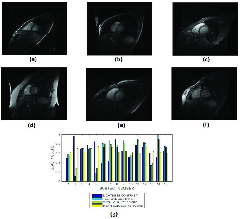
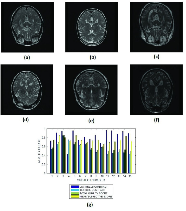
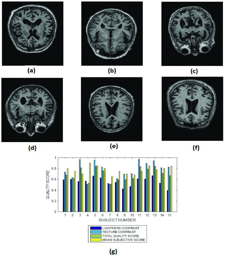
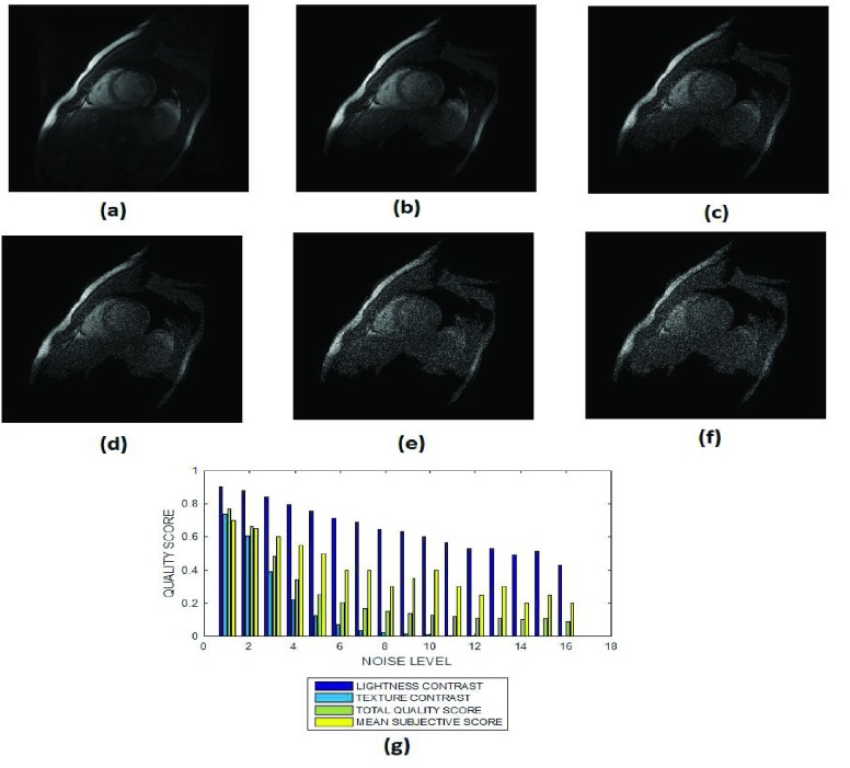
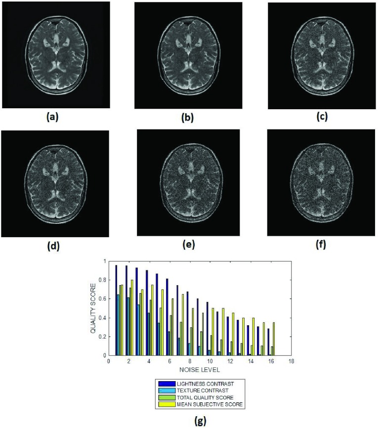
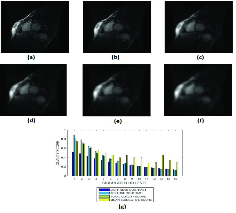
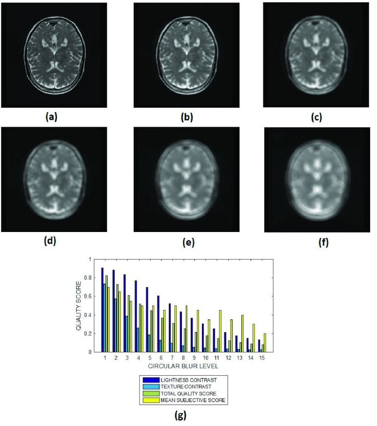
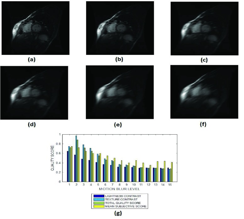
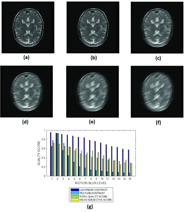
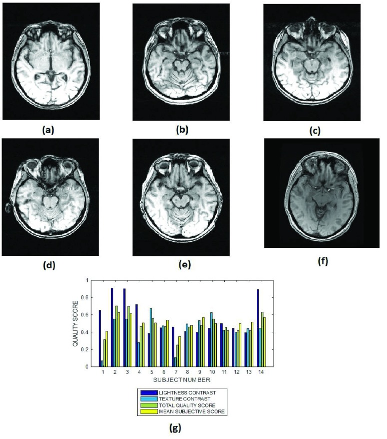
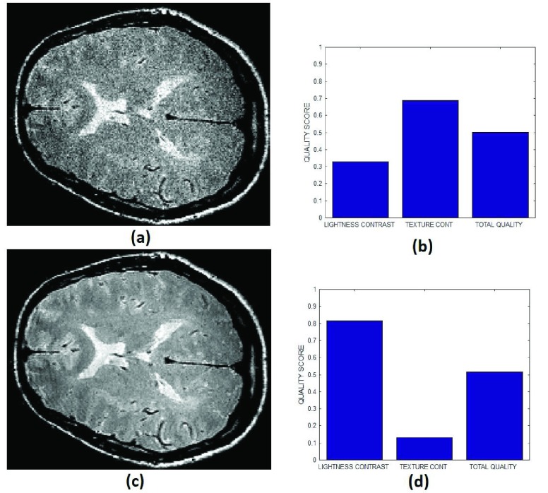
The objective performance evaluation of our proposed method is explained using six slices in each of Fig. 3 – Fig. 12. The mean subjective score assigned by the observers to each slice in a MRI volume data are displayed alongside the lightness contrast, texture contrast and total quality scores in Fig. 3g – Fig. 12g. Each figure except for Fig. 12, shows objective evaluation of a slice from MRI volume data of fifteen different subjects. In Fig. 12 the objective evaluation is on slices from 14 MRI volume data of different subjects. Cardiac, T2 and T1 brain MRI volume data without perceived degradation are displayed in Fig. 3, Fig.4 and Fig. 5, respectively. Different levels of Rician noise degradation on cardiac and T2 brain slices are displayed in Fig. 6 and Fig. 7, respectively. Figure 8 and Fig. 9 are images for the different levels of degradation by circular blur. Corresponding degradation by motion blur are displayed in Fig. 10 and Fig. 11. Quality assessment of MRI slices degraded by different configurations of bias fields are displayed in Fig. 12. Figure 13a is a T2 weighted brain MRI slice which was originally acquired with noise. The objective assessment by our proposed method is shown in Fig.13b. Figure 13c shows the same MRI slice after it was processed using noise removal algorithm proposed in [70] and [71]. The objective assessment by our proposed method after the noise removal is shown in Fig. 13d.

FIGURE 3.

Six slices from subject identification numbers (a) 2, (b) 5, (c) 7, (d) 10, (e) 12 and (f) 15 in a short axis cardiac MRI, (g) lightness contrast, texture contrast, total quality scores and the mean subjective scores of 15 slices from MRI volume data of different subjects.

FIGURE 4.

Six slices from subject identification numbers (a) 2, (b) 5, (c) 7, (d) 10, (e) 12 and (f) 15 in a T2 brain MRI volume data, (g) lightness contrast, texture contrast, total quality scores and the mean subjective scores of 15 slices from MRI volume data of different subjects.

FIGURE 5.

Six slices from subject identification numbers (a) 2, (b) 5, (c) 7, (d) 10, (e) 12 and (f) 15 in a T1 MPRAGE brain MRI volume data, (g) lightness contrast, texture contrast, total quality scores and the mean subjective scores of 15 slices from MRI volume data of different subjects.

FIGURE 6.

(a) A short axis cardiac MRI slice and its degraded versions at Rician noise levels (b) 3, (c) 7, (d) 9, (e) 12 and (g) 15 percent, (h) variation of the lightness contrast, texture contrast, total quality scores and the mean subjective scores with noise levels increasing from 1 to 15.

FIGURE 7.

(a) A T2-weighted brain MRI slice and its degraded versions at Rician noise levels (b) 3, (c) 7, (d) 9, (e) 12 and (g) 15 percent, (h) variation of the lightness contrast, texture contrast, total quality scores and the mean subjective scores with noise levels increasing from 1 to 15.

FIGURE 8.

(a) A short axis cardiac MRI slice and its degraded versions at circular blur levels (b) 3 voxels, (c) 7 voxels, (d) 9 voxels, (e) 12 voxels and (g) 15 voxels, (h) variation of the lightness contrast, texture contrast, total quality scores and the mean subjective scores with blur levels increasing from 1 to 15.

FIGURE 9.

(a) A T2 weighted brain MRI slice and its degraded versions at circular blur levels (b) 3 voxels, (c) 7 voxels, (d) 9 voxels, (e) 12 voxels and (g) 15 voxels, (h) variation of the lightness contrast, texture contrast, total quality scores and the mean subjective scores with blur levels increasing from 1 to 15.

FIGURE 10.

(a) A short axis cardiac MRI slice and its degraded versions at motion blur levels (b) 3, (c) 7, (d) 9, (e) 12 and (g) 15, (h) variation of the lightness contrast, texture contrast, total quality scores and the mean subjective scores with blur levels increasing from 1 to 15.

FIGURE 11.

(a) A T2 weighted brain MRI slice and its degraded versions at motion blur levels (b) 3, (c) 7, (d) 9, (e) 12 and (g) 15, (h) variation of the lightness contrast, texture contrast, total quality scores and the mean subjective scores with blur levels increasing from 1 to 15.

FIGURE 12.

Six slices from subject identification numbers (a) 1, (b) 5, (c) 7, (d) 9, (e) 11 and (f) 14 in a T1 brain MRI volume data degraded by different configurations of bias fields, (h) variation of the lightness contrast, texture contrast, total quality scores and the mean subjective scores of slices from 14 different MRI volume data.

FIGURE 13.

(a) An MRI slice originally acquired with noise, (b) texture contrast, lightness contrast and total quality scores of the noisy MRI slice, (c) the same MRI slice in (a) after post-acquisition processing with noise removal algorithm, (d) texture contrast, lightness contrast and total quality scores of the clean MRI slice in (c).

B. Subjective Validation

Validation of the proposed method through subjective evaluation by human observers are shown in Tables 1 – 7. On each table there are four columns under percentage difference score. Each column display the percentage of the 360 slices used for the subjective evaluation for which the percentage difference score lies within the range , , and .

TABLE 1. Analysis of PDS for Cardiac and Brain MRI Volume Data Without Perceived Degradation and Brain MRI Volume Data Degraded by Bias Fields.

Experiment Category	Number Slices	Percentage Difference Score
Cardiac MRI (No Degradation)	360	55	15	10	20
T2 Brain MRI (No Degradation)	360	70	10	5	15
MPRAGE Brain MRI (No Degradation)	360	73	12	5	10
T1 Brain MRI (Bias Fields)	360	65	10	8	17

TABLE 2. Analysis of PDS for Cardiac MRI Volume Data Degraded by Different Levels of Rician Noise.

Degradation Level	Number Slices	Percentage Difference Score
0	360	55	15	10	20
5	360	53	12	7	18
10	360	50	20	5	25
15	360	45	15	10	30

TABLE 3. Analysis of PDS for Cardiac MRI Volume Data Degraded by Different Levels of Circular Blur.

Degradation Level	Number Slices	Percentage Difference Score
0	360	55	15	10	20
5	360	50	15	10	25
10	360	52	12	9	27
15	360	47	15	12	26

TABLE 4. Analysis of PDS for Cardiac MRI Volume Data Degraded by Different Levels of Motion Blur.

Degradation Level	Number Slices	Percentage Difference Score
0	360	55	15	10	20
5	360	60	8	9	23
10	360	56	11	11	22
15	360	52	12	7	29

TABLE 5. Analysis of PDS for T2 Brain MRI Volume Data Degraded by Different Levels of Rician Noise.

Degradation Level	Number Slices	Percentage Difference Score
0	360	70	10	5	15
5	360	67	8	7	18
10	360	63	9	8	20
15	360	60	8	8	24

TABLE 6. Analysis of PDS for T2 Brain MRI Volume Data Degraded by Different Levels of Circular Blur.

Degradation Level	Number Slices	Percentage Difference Score
0	360	70	10	5	15
5	360	65	12	7	16
10	360	62	6	7	25
15	360	62	8	7	23

TABLE 7. Analysis of PDS for T2 Brain MRI Volume Data Degraded by Different Levels of Motion Blur.

Degradation Level	Number Slices	Percentage Difference Score
0	360	70	10	5	15
5	360	68	11	4	17
10	360	65	6	5	24
15	360	63	9	2	26

Table 1 are the results for cardiac and brain MRI volume data without perceived degradation and T1 volume data that were originally acquired with bias fields. Table 2 – Table 4 are the results for cardiac MRI volume data degraded by Rician noise, circular blur and motion blur, respectively. Table 5 – Table 7 are the results for T2 MRI volume data degraded by Rician noise, circular blur and motion blur, respectively. Table 8 show the variability in the scores assigned by the two observers in the subjective validation study.

TABLE 8. Inter-Rater Reliability Between Two Observers in the Ten Categories of the Subjective Validation Study.

Experiment Category	Inter-Rater Reliability
Cardiac MRI (No Degradation)	0.68
T2 Brain MRI (No Degradation)	0.73
MPRAGE Brain MRI (No Degradation)	0.80
T1 Brain MRI (Bias Fields)	0.75
Cardiac MRI (Rician Noise)	0.71
Cardiac MRI (Circular Blur)	0.65
Cardiac MRI (Motion Blur)	0.73
T2 Brain MRI (Rician Noise)	0.78
T2 Brain MRI (Circular Blur)	0.72
T2 Brain MRI (Motion Blur)	0.81

IV. Discussion

A. Evaluation Across Images Without Perceived Degradation

1). Cardiac MRI Images

The variations in the objective quality scores reflects differences in the perceived visual quality attributes of the cardiac MRI slices from the different MRI volume data. In Fig. 3 the endocardial and epicardial structures in the different slices are clearly visible relative to the background. The average lightness contrast quality score assigned to the slices is . This score reflects the high visibility of the foreground structures.

The constituent structures in the cardiac MRI slices have different clarity of details. Our proposed method predict texture contrast quality scores of 0.9 and 0.8 for MRI slices from subject number 7 (Fig. 3c) and subject number 12 (Fig. 3e), respectively. Lower texture contrast quality scores of 0.1 and 0.2 was predicted for MRI slices from subject number 2 (Fig. 3a) and subject number 5 (Fig. 3b), respectively. MRI slice from subject number 7 shown in Fig. 3c has better clarity of details than MRI slice from subject number 15 shown in Fig. 3f. Expectedly our proposed method predict a higher texture contrast quality score of 0.9 to the image in Fig. 3c and a lower texture contrast of 0.7 to the image in Fig. 3f.

2). T2 MRI Images

All the brain MRI images in Fig. 4 are quite visible relative to the background. The average lightness quality scores predicted for the 16 images is . The MRI slice from subject number 15 in Fig. 3f is visible relative to the background. However its clarity of details is much lower than the clarity of details in the slice from subject number 5 shown in Fig. 3b. Our proposed objective method can be said to be in agreement with visual perception. It assigns texture contrast quality score of 0.7 and 0.4 to the images in Fig. 3b and in Fig. 3f, respectively.

3). T1 MRI Images

The average lightness contrast quality score for the T1 MPRAGE images shown in Fig. 5 is . The lightness contrast for each slice is generally lower than the texture contrast quality score. The predicted objective scores can be attributed to the average intensity levels of the ventricular system and the cortical gray matter. The intensity levels of these major anatomical structures are similar to the background voxels. Thus the predicted lightness contrast quality score can be said to conform with visual perception.

The image in Fig. 5b reveals only the horn of the ventricle while the image in Fig. 5f reveals the main body of the ventricle. Our proposed method predict a lightness contrast quality score of 0.7 for the image in Fig. 5b. Lower lightness contrast quality score of 0.4 was predicted for the image in Fig. 5f. Visually the image in Fig. 5f has more clarity of details than the image in Fig. 5a. The predicted texture contrast quality scores for these images are 0.8 for Fig. 5f and 0.6 for Fig. 5a.

B. Evaluation Across Different Levels of Degradation

The images in Fig. 6a – Fig. 6f and the objective quality scores in Fig. 6g show that low level Rician noise can have severe effect on the contrast between the different anatomic structures in cardiac images. Beyond Rician noise level of 7 percent, the foreground is clearly visible from the background. However it becomes visually difficult to distinguish the boundaries between the endocardial and epicardial structures. Our proposed method effectively captures this visual perception. The lightness contrast quality score successively decrease from 0.9 to 0.5 for noise levels that increase from 0 percent to 15 percent. The texture contrast quality score decrease sharply from 0.75 to 0.15 for noise level that varies from 0 percent to 6 percent.

The ventricle and the cortical gray matter structures in the T2 images of Fig. 7 are more visible than the anatomic structures in the cardiac images in Fig. 6. The slope of the texture contrast quality score for the T2 images is lower than the slope of corresponding quality scores for the cardiac images shown in Fig. 6. This is an indication that Rician noise severely degrades cardiac images acquired using FIESTA protocol more than it does for T2 brain MRI images.

The lightness contrast, texture contrast and total quality scores successively decrease for circular blur (Fig. 8 and Fig. 9) and motion blur (Fig. 10 and Fig. 11) levels which increase from 0 to 15. The slope of the texture contrast quality score for the cardiac images in Fig. 10 is lower than corresponding quality score for the brain MRI images in Fig. 11. Visual inspection of the images show that the severity of degradation by motion blur on the cardiac images is less than those of the brain MRI images. These results are promising for the evaluation of images with different perceptual quality.

C. T1 MRI Images Degraded by Bias Fields

The different configurations of bias fields which degrade the images in Fig. 12 is reflected in the objective quality scores predicted by our proposed method. Images in Fig. 12b and 12c suffer from more severe bias fields than the other images shown in Fig. 12. Our proposed method predicts texture contrast quality score of 0.4 and 0.1, respectively for these images. The images in Fig. 12a and Fig. 12f can be considered as borderline cases because they suffer from mild bias fields. Our proposed method predict higher texture contrast quality scores of 0.57 and 0.5 for the images in Fig. 12a and Fig. 12f, respectively.

D. Practical Application in Clinical Environment

The images in Fig. 13 demonstrate practical application of our proposed method in a clinical environment for quality assessment of images. Figure 13a is a T2 weighted MRI image of a healthy brain acquired from a GE sigma scanner with a 1.5 Tesla magnet using spin echo mode. The image in Fig. 13c is the same image in Fig. 13a but have undergone processing for removal of Rician noise. There are several visual differences between the noisy image in Fig. 13a and the denoised image in Fig. 13c. The noisy image is darker in comparison to the denoised image and has low contrast between the cortical gray matter region and the white matter region. Our proposed method accurately assessed the difference in contrast by assigning lightness contrast quality scores of 0.32 and 0.8 to the noisy and denoised images, respectively. The image was denoised without significant blurring but it is very obvious that the texture features which was visible in the noisy image was eroded after processing. Thus, the predicted texture contrast quality score of 0.7 and 0.1 for the noisy and denoised image can be said to be in agreement with visual perception. The total quality score for both images appear to remain the same because the total quality score is heavily weighted towards texture contrast quality attribute.

E. Correlation With Subjective Evaluation by Human Observers

The validation results in Table 1 – Table 7 show that there is good correlation between our proposed objective method and the subjective score assigned by human observers. More than 70 percent of the slices used in all categories of the experiment have PDS less than 30 percent. The validation results show that for increasing levels of degradation there is a general decrease in percentage of slices with specific percentage difference scores. Thus it can be said that human observers tend to have better agreement at lower levels of degradation than at higher levels of degradation. Furthermore, the subjective evaluation by both human observers can be said to be reliable because the minimum and maximum inter-observer reliability are 0.61 and 0.81, respectively.

F. Interpretation of Objective Quality Scores

The threshold quality index for making decision on acceptable or non-acceptable image quality was fixed after due consultation with the human observers involved with the subjective evaluation experiments. There was consensus from both observers that texture contrast quality score should be the primary score for quality evaluation. Slices with texture contrast quality scores was recommended for visual examination. This is to determine if there is need for further reprocessing before any image analysis task can be carried out. The observers also recommended visual examination for slices with lightness contrast quality score of .

G. Computational Complexity

Our proposed method is computationally efficient. The normal distributions were built from central limit theorem unlike other approaches such as [42] and [72] which seek to build quality model from MRI volume data derived from large population. Quality evaluation steps such as intensity rescaling, feature extraction and computation of image moments are computed in a very simple method. Furthermore there is no need for additional resources such as image registration.

H. Limitations of Proposed Quality Assessment Method

The perceptual weight assigned for lightness contrast and texture contrast quality attributes was not optimal, but was derived in an ad hoc manner. The consequence is that the predicted total quality score may not correlate with the lightness and contrast quality attributes for different levels of degradation.

The proposed quality assessment method is designed to assess image quality based on four of several types of degradation processes. The degradation processes are circular blur, gaussian blur, Rician noise and intensity nonuniformity. Quality prediction does not incorporate variables from artifacts such as zebra stripes, chemical shift and aliasing as well as geometric and structural deformation of the MRI image. For this reason, the proposed quality assessment method will be suitable as an integral but fundamental part of a larger quality control system.

Quality prediction from the proposed method is a global approach which assumes that an MRI slice is homogeneous whereas MRI image, like most medical images are heterogenous. Thus quality prediction from the proposed method may not be a reliable assessment in clinical task where the focus is on specific anatomic structure. Examples are some task in clinical research such as atrophy measurement which requires quality assessment on specific anatomic structures of the brain; white matter, gray matter and ventricular system.

A simple but effective approach was adopted for foreground extraction. However, we acknowledge that our approach is not robust. It is more effective for brain MRI images than for cardiac MRI images. The basis of foreground extraction in the proposed method is the use of first moment as global threshold. The efficacy of our approach for foreground extraction decreases at high levels of noise.

Limited clinical data was a major logistic challenge during the research. At clinical research centers, degraded MRI images are further processed for quality enhancement as soon as they are detected. However, we had access to clinical MRI images with different configurations of intensity nonuniformity, but it was difficult to access real MRI images with different levels of circular blur, Gaussian blur and Rician noise degradation. Only retrospective MRI data without perceived degradation were available from the different sources. For this reason the degradation processes were modeled and artificially induced on real clinical data. Limited data makes it difficult to provide satisfactory statistical analysis which proves that our proposed method cover different processing requirements in clinical trials.

The limited number of readers and data are also to blame for the absence of robust statistical analysis of the validation study. We acknowledge that two statistical information was missing from the validation study. First there was is no information on the direction of the disagreement between the predicted objective quality scores and the subjective quality scores assigned by human observers. Second, there is no information on intra-reader variability as well as the predicted quality scores when the data were acquired.

I. Future Research Direction

In the future work we will address most limitations of our currently proposed method so that the improved algorithm can be play a significant role within a larger quality control system. We hope to develop robust foreground extraction algorithm and incorporate segmentation algorithm to allow the prediction of quality scores for specific region-of-interest within an MRI image. The quality variables will extend beyond classical quality attributes to include several types of artifacts and structural image quality attributes. Concerted effort will be made to recruit more readers for the subjective validation study. Relatively large clinical data with different levels of degradation will be acquired so that we can provide robust statistics analysis of the subjective validation study.

V. Conclusion

There is increasing clinical interest in the use of MRI images for the study of human anatomy, treatment and diagnosis of diseases. Currently MRI images are been considered the primary endpoints in large clinical trials of drugs for the treatment of neurological and cardiovascular diseases. In large clinical trials large volumes of MRI data are processed. Thus no-reference objective quality assessment is highly desired. The reliability of metric derived from quantitative analysis of MRI images is strongly dependent on rigorous monitoring throughout the various stages of the imaging workflow. We hereby propose a new method to evaluate the quality of brain MRI images from acquisition through processing to the analysis stages of the imaging workflow. Our proposed quality evaluation method re-evaluate and standardize the quality of MRI images acquired from different clinical trial sites across the globe and through all the stages of the imaging workflow. Experimental results demonstrates that our proposed method had good correlation with human visual judgment and gives fairly accurate quality evaluation within and across good quality images and different levels of degradation.

Funding Statement

This work was supported by the Alzheimer’s Disease Neuroimaging Initiative (ADNI) (National Institutes of Health) under Grant U01 AG024904 and the Department of Defense (DOD) ADNI under Grant W81XWH-12-2-0012. The work of M. Pedersen was supported by the Research Council of Norway through the ’IQMED: Image Quality enhancement in MEDical diagnosis, monitoring and treatment Project under Grant 247689.

References

- [1].Liney G., MRI in Clinical Practice. Springer, 2007. [Google Scholar]
- [2].Yankeelov T. E. and Gore J. C., “Dynamic contrast enhanced magnetic resonance imaging in oncology: Theory, data acquisition, analysis, and examples,” Current Med. Imag. Rev., vol. 3, no. 2, pp. 91–107, 2007. [DOI] [PMC free article] [PubMed] [Google Scholar]
- [3].Fazekas F.et al. , “The contribution of magnetic resonance imaging to the diagnosis of multiple sclerosis,” Neurology, vol. 53, no. 3, p. 448, 1999. [DOI] [PubMed] [Google Scholar]
- [4].Teipel S. J.et al. , “Anatomical MRI and DTI in the diagnosis of Alzheimer’s disease: A European multicenter study,” J. Alzheimer’s Disease, vol. 31, no. s3, pp. S33–S47, 2012. [DOI] [PubMed] [Google Scholar]
- [5].Khoury S. J.et al. , “ACCLAIM: A randomized trial of abatacept (CTLA4-Ig) for relapsing-remitting multiple sclerosis,” Multiple Sclerosis J., vol. 23, no. 5, pp. 686–695, 2016. [DOI] [PMC free article] [PubMed] [Google Scholar]
- [6].Gold R.et al. , “Long-term effects of delayed-release dimethyl fumarate in multiple sclerosis: Interim analysis of ENDORSE, a randomized extension study,” Multiple Sclerosis J., vol. 23, no. 2, pp. 253–265, 2016. [DOI] [PMC free article] [PubMed] [Google Scholar]
- [7].Maranzano J., Rudko D. A., Arnold D. L., and Narayanan S., “Manual segmentation of ms cortical lesions using MRI: A comparison of 3 MRI reading protocols,” Amer. J. Neuroradiol., vol. 37, no. 9, pp. 1623–1628, 2016. [DOI] [PMC free article] [PubMed] [Google Scholar]
- [8].Lu H., Nagae-Poetscher L. M., Golay X., Lin D., Pomper M., and van Zijl P. C. M., “Routine clinical brain MRI sequences for use at 3.0 tesla,” J. Magn. Reson. Imag., vol. 22, no. 1, pp. 13–22, 2005. [DOI] [PubMed] [Google Scholar]
-
[9].Arnold D. L.et al. , “Superior mri outcomes with alemtuzumab compared with subcutaneous interferon
-1a in MS,” Neurology, vol. 87, no. 14, pp. 1464–1472, 2016. [DOI] [PMC free article] [PubMed] [Google Scholar]
- [10].Kappos L.et al. , “Daclizumab HYP versus interferon beta-1a in relapsing multiple sclerosis,” New England J. Med., vol. 373, no. 15, pp. 1418–1428, 2015. [DOI] [PubMed] [Google Scholar]
- [11].De Stefano N. and Arnold D. L., “Towards a better understanding of pseudoatrophy in the brain of multiple sclerosis patients,” Multiple Sclerosis J., vol. 21, no. 6, pp. 675–676, 2015. [DOI] [PubMed] [Google Scholar]
- [12].Nakamura K., Guizard N., Fonov V. S., Narayanan S., Collins D. L., and Arnold D. L., “Jacobian integration method increases the statistical power to measure gray matter atrophy in multiple sclerosis,” NeuroImage, Clin., vol. 4, pp. 10–17, Jan. 2014. [DOI] [PMC free article] [PubMed] [Google Scholar]
- [13].Banwell B.et al. , “MRI in the evaluation of pediatric multiple sclerosis,” Neurology, vol. 87, no. 9, pp. S88–S96, 2016. [DOI] [PubMed] [Google Scholar]
- [14].Makhani N.et al. , “Viral exposures and MS outcome in a prospective cohort of children with acquired demyelination,” Multiple Sclerosis J., vol. 22, no. 3, pp. 385–388, 2016. [DOI] [PubMed] [Google Scholar]
- [15].Kappos L.et al. , “Safety and efficacy of amiselimod in relapsing multiple sclerosis (MOMENTUM): A randomised, double-blind, placebo-controlled phase 2 trial,” Lancet Neurol., vol. 15, no. 11, pp. 1148–1159, 2016. [DOI] [PubMed] [Google Scholar]
- [16].Cohen J. A.et al. , “Safety and efficacy of the selective sphingosine 1-phosphate receptor modulator ozanimod in relapsing multiple sclerosis (RADIANCE): A randomised, placebo-controlled, phase 2 trial,” Lancet Neurol., vol. 15, no. 4, pp. 373–381, 2016. [DOI] [PubMed] [Google Scholar]
- [17].Bogachkov A.et al. , “Right ventricular assessment at cardiac MRI: Initial clinical experience utilizing an is-sense reconstruction,” Int. J. Cardiovascular Imag., vol. 32, no. 7, pp. 1081–1091, 2016. [DOI] [PubMed] [Google Scholar]
- [18].Rayoo R.et al. , “Cardiac MRI: Indications and clinical utility—A single centre experience,” Heart, Lung Circulat., vol. 21, p. S191, Jan. 2012. [Google Scholar]
- [19].Stokes M. B., Nerlekar N., Moir S., and Teo K. S., “The evolving role of cardiac magnetic resonance imaging in the assessment of cardiovascular disease,” Austral. Family Phys., vol. 45, no. 10, pp. 761–764, 2016. [PubMed] [Google Scholar]
- [20].Bhatti S.et al. , “Clinical and prognostic utility of cardiovascular magnetic resonance imaging in myeloma patients with suspected cardiac amyloidosis,” Eur. Heart J.-Cardiovascular Imag., vol. 17, no. 9, pp. 970–977, 2016. [DOI] [PubMed] [Google Scholar]
- [21].Rickers C.et al. , “Utility of cardiac magnetic resonance imaging in the diagnosis of hypertrophic cardiomyopathy,” Circulation, vol. 112, no. 6, pp. 855–861, 2005. [DOI] [PubMed] [Google Scholar]
- [22].He X. and Park S., “Model observers in medical imaging research,” Theranostics, vol. 3, no. 10, pp. 774–786, 2013. [DOI] [PMC free article] [PubMed] [Google Scholar]
- [23].Barrett H. H., Myers K. J., Hoeschen C., Kupinski M. A., and Little M. P., “Task-based measures of image quality and their relation to radiation dose and patient risk,” Phys. Med. Biol., vol. 60, no. 2, p. R1, 2015. [DOI] [PMC free article] [PubMed] [Google Scholar]
- [24].Kupinski M. A., Hoppin J. W., Clarkson E., and Barrett H. H., “Ideal-observer computation in medical imaging with use of Markov-chain Monte Carlo techniques,” J. Opt. Soc. Amer. A, Opt. Image Sci., vol. 20, no. 3, pp. 430–438, 2003. [DOI] [PMC free article] [PubMed] [Google Scholar]
- [25].Pizurica A., Philips W., Lemahieu I., and Acheroy M., “A versatile wavelet domain noise filtration technique for medical imaging,” IEEE Trans. Med. Imag., vol. 22, no. 3, pp. 323–331, Mar. 2003. [DOI] [PubMed] [Google Scholar]
- [26].Axel L. and Dougherty L., “MR imaging of motion with spatial modulation of magnetization,” Radiology, vol. 171, no. 3, pp. 841–845, 1989. [DOI] [PubMed] [Google Scholar]
- [27].Ordidge R. J., Helpern J. A., Qing Z. X., Knight R. A., and Nagesh V., “Correction of motional artifacts in diffusion-weighted MR images using navigator echoes,” Magn. Reson. Imag., vol. 12, no. 3, pp. 455–460, 1994. [DOI] [PubMed] [Google Scholar]
- [28].Caramanos Z.et al. , “Gradient distortions in MRI: Characterizing and correcting for their effects on SIENA-generated measures of brain volume change,” NeuroImage, vol. 49, no. 2, pp. 1601–1611, 2010. [DOI] [PubMed] [Google Scholar]
- [29].Zhu Y., Zhai G., Gu K., and Zhu W., “No-reference quality assessment for JPEG compressed images,” in Proc. 9th Int. Conf. Qual. Multimedia Exper. (QoMEX), May/Jun. 2017, pp. 1–6. [Google Scholar]
- [30].Knaus C. and Zwicker M., “Dual-domain image denoising,” in Proc. 20th IEEE Int. Conf. Image Process. (ICIP), Sep. 2013, pp. 440–444. [Google Scholar]
- [31].Marziliano P., Dufaux F., Winkler S., and Ebrahimi T., “Perceptual blur and ringing metrics: Application to JPEG2000,” Signal Process., Image Commun., vol. 19, no. 2, pp. 163–172, 2004. [Google Scholar]
- [32].Buades A., Coll B., and Morel J.-M., “A non-local algorithm for image denoising,” in Proc. IEEE Comput. Soc. Conf. Comput. Vis. Pattern Recognit. (CVPR), vol. 2, Jun. 2005, pp. 60–65. [Google Scholar]
- [33].De Stefano N.et al. , “Assessing brain atrophy rates in a large population of untreated multiple sclerosis subtypes,” Neurology, vol. 74, no. 23, pp. 1868–1876, 2010. [DOI] [PubMed] [Google Scholar]
- [34].Krupinski E. A., “The importance of perception research in medical imaging,” Radiat. Med., vol. 18, no. 6, pp. 329–334, 2000. [PubMed] [Google Scholar]
- [35].Robinson R.et al. , “Automatic quality control of cardiac MRI segmentation in large-scale population imaging,” in Proc. Int. Conf. Med. Image Comput. Comput.-Assisted Intervent. Cham, Switzerland: Springer, 2017, pp. 720–727. [Google Scholar]
- [36].Chow L. S. and Paramesran R., “Review of medical image quality assessment,” Biomed. Signal Process. Control, vol. 27, no. 1, pp. 145–154, 2016. [Google Scholar]
- [37].Chalavi S., Simmons A., Dijkstra H., Barker G. J., and Reinders A. A. T. S., “Quantitative and qualitative assessment of structural magnetic resonance imaging data in a two-center study,” BMC Med. Imag., vol. 12, no. 1, p. 27, 2012. [DOI] [PMC free article] [PubMed] [Google Scholar]
- [38].de Certaines J. D. and Cathelineau G., “Safety aspects and quality assessment in MRI and MRS: A challenge for health care systems in Europe,” J. Magn. Reson. Imag., vol. 13, no. 4, pp. 632–638, 2001. [DOI] [PubMed] [Google Scholar]
- [39].Mortamet B.et al. , “Automatic quality assessment in structural brain magnetic resonance imaging,” Magn. Reson. Med., vol. 62, no. 2, pp. 365–372, 2009. [DOI] [PMC free article] [PubMed] [Google Scholar]
- [40].Woodard J. P. and Carley-Spencer M. P., “No-reference image quality metrics for structural MRI,” Neuroinformatics, vol. 4, no. 3, pp. 243–262, 2006. [DOI] [PubMed] [Google Scholar]
- [41].Osadebey M., Pedersen M., Arnold D., and Wendel-Mitoraj K., “No-reference quality measure in brain MRI images using binary operations, texture and set analysis,” IET Image Process., vol. 11, no. 9, pp. 672–684, 2017. [Google Scholar]
- [42].Osadebey M., Pedersen M., Arnold D., and Wendel-Mitoraj K., “Bayesian framework inspired no-reference region-of-interest quality measure for brain MRI images,” J. Med. Imag., vol. 4, no. 2, p. 025504, 2017. [DOI] [PMC free article] [PubMed] [Google Scholar]
- [43].Osadebey M. E., Pedersen M., Arnold D., and Wendel-Mitoraj K., “The spatial statistics of structural magnetic resonance images: Application to post-acquisition quality assessment of brain MRI images,” Imag. Sci. J., vol. 65, no. 8, pp. 468–483, 2017. [Google Scholar]
- [44].Rosen A.et al. , “Data-driven assessment of structural image quality,” NeuroImage, 2017. [DOI] [PMC free article] [PubMed]
- [45].Esteban O., Birman D., Schaer M., Koyejo O. O., Poldrack R. A., and Gorgolewski K. J., “MRIQC: Advancing the automatic prediction of image quality in MRI from unseen sites,” PLoS ONE, vol. 12, no. 9, p. e0184661, 2017. [DOI] [PMC free article] [PubMed] [Google Scholar]
- [46].Reuter M., Tisdall M. D., Qureshi A., Buckner R. L., van der Kouwe A. J. W., and Fischl B., “Head motion during MRI acquisition reduces gray matter volume and thickness estimates,” NeuroImage, vol. 107, pp. 107–115, Feb. 2015. [DOI] [PMC free article] [PubMed] [Google Scholar]
- [47].Alexander-Bloch A.et al. , “Subtle in-scanner motion biases automated measurement of brain anatomy from in vivo MRI,” Hum. Brain Mapping, vol. 37, no. 7, pp. 2385–2397, 2016. [DOI] [PMC free article] [PubMed] [Google Scholar]
- [48].Pardoe H. R., Hiess R. K., and Kuzniecky R., “Motion and morphometry in clinical and nonclinical populations,” NeuroImage, vol. 135, pp. 177–185, Jul. 2016. [DOI] [PubMed] [Google Scholar]
- [49].Moraru L., Moldovanu S. S., and Obreja C. D., “A survey over image quality analysis techniques for brain MR images,” Int. J. Radiol., vol. 2, no. 1, pp. 24–28, 2015. [Google Scholar]
- [50].Cavaro-Menard C., Zhang L., and Le Callet P., “Diagnostic quality assessment of medical images: Challenges and trends,” in Proc. 2nd Eur. Workshop Vis. Inf. Process. (EUVIP), Jul. 2010, pp. 277–284. [Google Scholar]
- [51].Mathews T. and Smith M. R., “Objective image quality measures for evaluating advanced MRI reconstruction methods,” in Proc. Can. Conf. Elect. Comput. Eng., vol. 1, 1996, pp. 359–361. [Google Scholar]
- [52].Lauzon C. B., Caffo B. C., and Landman B. A., “Towards automatic quantitative quality control for MRI,” Proc. SPIE, vol. 8314, p. 83140K, Feb. 2012. [DOI] [PMC free article] [PubMed] [Google Scholar]
- [53].Kellman P. and McVeigh E. R., “Image reconstruction in SNR units: A general method for SNR measurement,” Magn. Reson. Med., vol. 54, no. 6, pp. 1439–1447, 2005. [DOI] [PMC free article] [PubMed] [Google Scholar]
- [54].Rajan J., Poot D., Juntu J., and Sijbers J., “Noise measurement from magnitude MRI using local estimates of variance and skewness,” Phys. Med. Biol., vol. 55, no. 16, p. N441, 2010. [DOI] [PubMed] [Google Scholar]
- [55].Aja-Fernández S., Tristán-Vega A., and Alberola-López C., “Noise estimation in single- and multiple-coil magnetic resonance data based on statistical models,” Magn. Reson. Imag., vol. 27, no. 10, pp. 1397–1409, 2009. [DOI] [PubMed] [Google Scholar]
- [56].Andreopoulos A. and Tsotsos J. K., “Efficient and generalizable statistical models of shape and appearance for analysis of cardiac MRI,” Med. Image Anal., vol. 12, no. 3, pp. 335–357, 2008. [DOI] [PubMed] [Google Scholar]
- [57].Zhang Y., Brady M., and Smith S., “Segmentation of brain MR images through a hidden Markov random field model and the expectation-maximization algorithm,” IEEE Trans. Med. Imag., vol. 20, no. 1, pp. 45–57, Jan. 2001. [DOI] [PubMed] [Google Scholar]
- [58].Tsai W.-H., “Moment-preserving thresolding: A new approach,” Comput. Vis., Graph., Image Process., vol. 29, no. 3, pp. 377–393, 1985. [Google Scholar]
- [59].Campisi P. and Egiazarian K., Blind Image Deconvolution: Theory and Applications. Boca Raton, FL, USA: CRC Press, 2007. [Google Scholar]
- [60].Wilkinson M. H. F. and Schut F., Digital Image Analysis of Microbes: Imaging, Morphometry, Fluorometry and Motility Techniques and Applications. Hoboken, NJ, USA: Wiley, 1998. [Google Scholar]
- [61].Li S. Z., Markov Random Field Modeling in Image Analysis. Springer, 2009. [Google Scholar]
- [62].Flusser J. and Suk T., “Degraded image analysis: An invariant approach,” IEEE Trans. Pattern Anal. Mach. Intell., vol. 20, no. 6, pp. 590–603, Jun. 1998. [Google Scholar]
- [63].van der Schaaf A. and van Hateren J. H., “Modelling the power spectra of natural images: Statistics and information,” Vis. Res., vol. 36, no. 17, pp. 2759–2770, 1996. [DOI] [PubMed] [Google Scholar]
- [64].Grafarend E. W., Linear and Nonlinear Models: Fixed Effects, Random Effects, and Mixed Models. Berlin, Germany: Walter de Gruyter, 2006. [Google Scholar]
- [65].Lee J.-S., “Digital image enhancement and noise filtering by use of local statistics,” IEEE Trans. Pattern Anal. Mach. Intell., vol. PAMI-2, no. 2, pp. 165–168, Feb. 1980. [DOI] [PubMed] [Google Scholar]
- [66].Van Ngo K., Storvik J. J., Dokkeberg C. A., Farup I., and Pedersen M., “QuickEval: A Web application for psychometric scaling experiments,” Proc. SPIE, vol. 9396, p. 93960O, Feb. 2015. [Google Scholar]
- [67].Gedamu E. L., Collins D. L., and Arnold D. L., “Automated quality control of brain MR images,” J. Magn. Reson. Imag., vol. 28, no. 2, pp. 308–319, 2008. [DOI] [PubMed] [Google Scholar]
- [68].Streijl R. C., Winkler S., and Hands D. S., “Mean opinion score (MOS) revisited: Methods and applications, limitations and alternatives,” Multimedia Syst., vol. 22, no. 2, pp. 213–227, 2016. [Google Scholar]
- [69].Delcourt C., Cubeau J., Balkau B., and Papoz L., “Limitations of the correlation coefficient in the validation of diet assessment methods,” Epidemiology, vol. 5, no. 5, pp. 518–524, 1994. [PubMed] [Google Scholar]
- [70].Garnier S. J., Bilbro G. L., Gault J. W., and Snyder W. E., “Magnetic resonance image restoration,” J. Math. Imag. Vis., vol. 5, no. 1, pp. 7–19, 1995. [Google Scholar]
- [71].Garnier S. J., Bilbro G. L., Snyder W. E., and Gault J. W., “Noise removal from multiple MRI images,” J. Digit. Imag., vol. 7, no. 4, p. 183, 1994. [DOI] [PubMed] [Google Scholar]
- [72].Fang Y., Ma K., Wang Z., Lin W., Fang Z., and Zhai G., “No-reference quality assessment of contrast-distorted images based on natural scene statistics,” IEEE Signal Process. Lett., vol. 22, no. 7, pp. 838–842, Jul. 2015. [Google Scholar]