GPU Accelerated Multilevel Lagrangian Carotid Strain Imaging

Abstract

A multi-level Lagrangian carotid strain imaging algorithm is analyzed to identify computational bottlenecks for implementation on a Graphics Processing Unit (GPU). Displacement tracking including regularization was found to be the most computationally expensive aspect of this strain imaging algorithm taking about 2.2 hours for an entire cardiac cycle. This intensive displacement tracking was essential to obtain Lagrangian strain tensors. However, most of the computational techniques used for displacement tracking are parallelizable and hence GPU implementation is expected to be beneficial. A new scheme for sub-sample displacement estimation referred to as a multi-level global peak finder (MLGPF) was also developed since the Nelder–Mead simplex optimization technique used in the CPU implementation was not suitable for GPU implementation. GPU optimizations to minimize thread divergence, utilization of shared and texture memory were also implemented. This enables efficient use of the GPU computational hardware and memory bandwidth. Overall, an application speedup of 168.75X was obtained enabling the algorithm to finish in about 50 secs for a cardiac cycle. Lastly, comparison of GPU and CPU implementations demonstrated no significant difference in the quality of displacement vector and strain tensor estimation with the two implementations upto a five percent inter frame deformation. Hence, a GPU implementation is feasible for clinical adoption and opens opportunity for other computationally intensive techniques.

I. Introduction

ULTRASOUND strain imaging [1] is a modality which provides information about mechanical properties of tissues. This modality has been used for several non-invasive clinical diagnostic applications over the last decade. For example, quasi static breast strain imaging has been used to both detect and discriminate between benign and malignant breast lesions [2]. Several researchers have also shown the usefulness of carotid strain imaging in vivo as it can predict plaque vulnerability [3–9].

Carotid strain imaging is implemented using the natural cardiac pulsation of the carotid arteries as stimuli. Along longitudinal views the effect is such that motion of the near wall and far wall of the artery are in opposite directions as the artery expands and contracts. This inherent discontinuous motion makes the task of estimating the displacement map for carotid strain imaging a challenging one[10]. In addition, there may be additional physiological motion which causes both walls to move differently.

Recently, Graphics Processor Units (GPUs) have been used in strain imaging to allow for faster computational and processing efficiency. NVIDIA (Santa Clara, CA) has introduced CUDA (Compute Unified Device Architecture) which is a parallel programming platform allowing easy programming of GPUs. Idzenga et al. [11] identified that about 90% of their strain imaging algorithm computation time was spent in performing Normalized Cross Correlation (NCC) computations and hence implemented NCC on a GPU using CUDA. Verma and Doyley[12] used a GPU to perform beam forming and two-dimensional (2D) cross correlation and achieved frame rates 400 times faster than conventional methods. Rosenzweig et al. [13] implemented acoustic radiation force impulse (ARFI) imaging on GPU, to improve the efficiency of cubic spline interpolation and Loupas 2-D autocorrelator [14]. Yang et al. [15] implemented a hybrid CPU-GPU strain imaging algorithm using 1D cross correlation where median filtering of displacement estimates and strain estimation was done on the CPU for a previous frame while the remaining compute intensive calculations were done on GPU for the current frame in parallel. Recently, Peng et al. [16] implemented a 3D coupled sub-sample estimation algorithm for breast elastography using GPU. This was accomplished by using a K20 NVIDIA GPU to obtain a 3D cross-correlation map which was up-sampled using spline interpolation with marching-cube algorithm [17] and then fitted to an ellipsoidal model to estimate the final displacements [18, 19].

Lagrangian carotid strain imaging is generally performed using the following steps. First, a cumulative displacement vector map obtained based on the inter-frame displacements estimated is generated. Second, accumulated displacement vectors are obtained prior to the estimation of the corresponding accumulated strain tensors. Then, the gradient of the displacement vectors is used for calculating the local strain tensors. The first step can be viewed as a deformable registration problem and possible solutions are block matching methods [20, 21]. In these methods blocks of data are matched between consecutive frames using a similarity measure such as NCC. To form the displacement map accurately, Shi et al. [10] used a multi-level pyramid scheme where coarser blocks of data are used to initialize search regions for higher levels that use finer blocks to improve spatial resolution. Multilevel block matching has allowed for accurate calculation of discontinuous displacement maps. Here strain calculated at lower levels can be used to scale the data at higher levels to reduce signal decorrelation and enhance accuracy of displacement estimation [22, 23]. Block matching methods however do not utilize global information and hence can be susceptible to signal decorrelation and peak hopping errors. In order to address this problem, McCormick et al. [24] used a Bayesian regularization approach where displacement estimates from neighboring blocks are used as a prior to aid accurate displacement estimation. The amount of deformation per frame can be small and micrometer precision is desired, hence subsample displacement estimation is necessary. McCormick et al. [25] used a 2D windowed sinc interpolator to enable accurate and precise subsample displacement vector estimation. The techniques developed in [10, 22–25] have been combined together in [6] and have successfully shown to quantify carotid plaque instability.

Since, the strain imaging algorithm described in [6] is a combination of techniques developed over the years, the improved quality observed in the strain maps formed comes at the cost of significantly increased computation time. Moreover, for carotid strain imaging, displacements accumulated over an entire cardiac cycle and corresponding accumulated strain estimation are required to characterize plaque vulnerability. Here around 25 frames of data over a cardiac cycle have to be processed which takes around two hours with the current algorithm on a single-threaded CPU [6]. In this work, we implement the algorithm presented in [6] on a GPU to allow for faster processing and hence making this approach feasible for clinical adoption.

This work reports on two main contributions. First, we quantify computation time for the different techniques which have been incorporated to our strain imaging algorithm. Second, we implement these algorithms on a GPU without loss of image quality and demonstrate the speedup in processing time making the algorithm feasible in a clinical setting. In this process we redesigned algorithms to make them suitable for GPU computing and explored standard optimizations for the same.

II. Materials And Methods

An Intel(R) Xeon(R) CPU E5–2640 v4 @ 2.40GHz was used to run the algorithm. The GPU used was a Tesla K40c which belongs to the Kepler architecture with compute capability 3.5. The original algorithm was implemented in C++ using the Insight Toolkit (ITK) library [26]. CPU multithreading was not used. Table I presents the different stages used in the original algorithm which will be discussed in the following paragraphs.

Table I.

Abbreviations of Computation stages

Abbreviation	Stage Name
UPMD	Upsample and Prepare Multilevel Data
DU	Data Update
AT	Affine Transform
CH	Correlation Helper
NCC	Normalized Cross-Correlation
RC	Regularization Calculation
SDC	Subsample Displacement Calculation

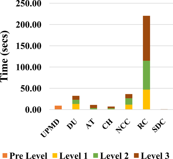
Computational bottlenecks in the original implementation by McCormick et al. [27] were first identified. A timing analysis for a single inter-frame displacement calculation with this algorithm is presented in Fig. 1. These inter-frame displacement computation stages take a total of 317.25 secs per frame pair. The next step is displacement accumulation and strain tensor calculation. This is done after plaque segmentation and hence the time taken for this step varies depending on the plaque size. Our timing analysis on a carotid wall segmentation versus a large plaque segmentation shows that this took between 2.38 secs and 3.07 secs per frame pair respectively. This time includes the time spent in writing out the data to files with each plaque pixel location and corresponding strain values. However, this is very small compared to the 317.25 secs taken for displacement estimation and hence we focus on speeding up the displacement estimation process.

Fig. 1.

Timing analysis of original CPU implementation

We use the term current image and next image to describe the initial and second frame that is used in inter-frame displacement estimation respectively. The Up-sample and Prepare Multi-level Data (UPMD) stage calculates the current and next images that will be used by the three levels of the multi-level displacement estimation algorithm. Note that these images are sampled differently for each level. First a windowed sinc interpolator is used to up-sample the original current and next image by a factor of 2 in both the axial and lateral direction. Following this up sampling the decimation factors presented in Table II are applied since the lower levels are operated at a coarser granularity to improve computational speed and reduce erroneous displacement tracking. Higher decimation is allowed in the axial direction after conversion to envelope signals (to satisfy Nyquist criterion) since we have higher resolution in that direction. Following the decimation Gaussian smoothing is applied which allows for derivative operations to be applied without singularities.

Table II.

Decimation Factors

Level	Lateral Decimation	Axial Decimation
1	2	3
2	1	2
3	1	1

The Data Update (DU) stage is used to load the appropriate current and next image before proceeding to further stages for a given level. The Affine Transform (AT) stage is used only for level 2 and level 3 where the current image blocks are scaled according to strain observed in previous levels as discussed in [22, 23]. The Correlation Helper (CH) and the normalized cross-correlation (NCC) stages perform NCC of data blocks from current image to search regions in the next image. For performing NCC, the mean and variances of data block being cross-correlated are required. These values are calculated in the CH stage and hence it is a helper to the NCC stage. The radius and size of the data blocks formed from the current images along with the search region ratios and resulting NCC matrix sizes are shown in Table III. The data block size is calculated as 2∗radius+1. The NCC matrix sizes are calculated as 2 ∗ ceil(search ratio ∗ radius)+ 1. The last column determines the number of NCC operations performed of the current image data block to different offsets of the same sized block in the next image. The essence of multi-level tracking is having large data block sizes at the lower levels accompanied with a large search region as one is less likely to generate false positives with a large data block size. However, the resolution of displacement vectors generated is low with large blocks. Hence the displacement vectors from the lower levels are simply used to guide the search region initialization of the higher levels which perform NCC at smaller block sizes to achieve high spatial resolution for the displacement vectors.

Table III.

Block Sizes [Lateral, Axial]

Level	Block Radius	Block Size	Search Ratio	NCC Matrix Size
1	[15,28]	[31,57]	[2.2,1.4]	[67, 81]
2	[12,23]	[25,47]	[1.65,1.25]	[41,59]
3	[10,18]	[21,37]	[1.1, 1.1]	[23,41]

The RC stage performs a Bayesian regularization process on the NCC matrices and is described in detail in [24]. The key process is, given a NCC matrix, use corresponding values from left, right, top and bottom NCC matrices to remove noisy NCC values in the given matrix. This is an iterative process and three iterations have been found to be sufficient to reduce noise in the estimation. Following this the regularized NCC matrices were used to form the displacement vectors. To accurately estimate the displacement vector, subsample displacement calculation (SDC) [25, 28] is done using interpolation. A simple parabolic interpolation is used for the level 1 and level 2 while the final level uses a 2D windowed sinc interpolation; a reconstructive method that does not have a closed form expression for the peak, but provides unbiased and accurate subsample estimates. The CPU implementation for sinc interpolation uses a Nelder-Mead simplex optimization to find this peak [25].

A. GPU Version 1

To implement this algorithm on a GPU, we first identified bottlenecks of the original ITK algorithm. Figure 1 illustrates that Bayesian regularization was the main bottleneck. The next bottleneck being the CH and NCC stage together. We initially implemented these three stages on the GPU with the frames copied to the GPU before the CH stage and the regularized matrices copied back to the CPU after the RC stage. The improved computational results were presented at a conference where Meshram et al. .()[29] reported an application speedup of 13.75X. In this paper we implement all the remaining stages of the algorithm on the GPU and hence achieve a significantly faster implementation with higher speedup.

Data movement between GPU and CPU memory in the final implementation is as follows. The current and next frames are copied to the GPU memory before the computational stages. After the end of SDC stage in each level displacement estimates are copied back to CPU memory and used to initialize offsets for the NCC search region for the next level. These offsets are copied to the GPU memory from the CPU memory at the beginning of each NCC stage. For the final level the displacement estimates generated are the final results for the given frame pair and the algorithm moves on to the next frame pair. The GPU implementation of the UPMD stage performs up sampling using windowed sinc interpolation. Following this it performs the appropriate decimation and smoothening of the images and stores the resulting images for all three levels in GPU memory. The DU stage was not required for GPU implementation and hence was removed.

RF data from the Siemens S2000 system is stored in a signed short format which is a 2-byte format. However, in order to reduce any quantization errors in the up sampling stage we moved to a single precision floating point format which is a 4-byte format. This makes the GPU NCC stage more computationally expensive when compared to the corresponding CPU stage.

The current GPU images are then used as input for the AT stage for level 2 and level 3 which generates, transformed current image data blocks based on the strain computed in prior levels. The data blocks are formed from the original current image for level 1. The size of these data blocks are presented in column 3 of Table III. The CH stage is now used only for setting up offsets for search regions based on displacements computed in prior levels. The CH stage was relieved of calculating the mean and variances of data blocks as this is now done in the NCC stage itself. The NCC stage forms the NCC matrices which are stored in GPU memory. The size of the NCC matrices formed is presented in column 5 of Table III.

The NCC matrices are then regularized in the RC stage. Following this a parallel reduction operation is performed on the regularized NCC matrices to find the maximum NCC value. An optimized GPU based reduction algorithm presented by Harris [30] was used for this purpose. For level 1 and 2 parabolic interpolation was performed using the maximum NCC value and its neighbors [28]. For level 3, the CPU implementation used the Nelder-Mead simplex optimization to interpolate the peak in the NCC matrix using 2D windowed sinc interpolation. Although this process can be done in parallel for each NCC matrix, enough data blocks do not exist to make this approach suitable for CUDA. Hence an alternate approach that works efficiently on a GPU namely a multi-level global peak finder (MLGPF) was implemented.

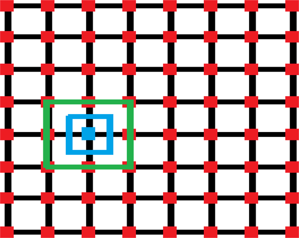
MLGPF starts with finding the maximum or peak NCC value. Following this we set a region around this maximum which ranges from the matrix element prior to the maximum and ends at matrix element after the maximum. When done in 2D this approach forms a rectangular region. A grid is formed in this region and a 2D windowed sinc interpolator is utilized to compute in parallel with multiple threads as shown by red points in Fig. 2. Figure 2 shows how this process was performed with 64 threads. Our initial attempt with MLGPF used 1024 threads to generate a finer grid. Following this, we again use the Harris [30] reduction approach to find the maximum of all grid points. After this, the process is repeated with a smaller region around the new interpolated maximum. For the first step where the sampling distance is large we use a relaxed shrinking factor shown in green in Fig. 2 for the new region because the actual global peak may be closer to another grid point than the one we calculated as the maximum to avoid any jitter errors. However, once we have a small search region we are less likely to miss the global peak and hence we can use a tighter shrinking factor shown in blue. Thus, relaxed shrinking was used only for the first iteration and tighter shrinking used for further iterations. Five iterations of the algorithm with 1024 samples in each iteration were found to match or exceed the subsample peak computed using the Nelder-Mead simplex optimization approach. If we consider the distance between neighboring values in the estimation/ interpolation matrix as a single unit. The relaxed shrinking factor denotes two units (one unit in each direction) and the tight shrinking factor represents one unit (half unit in each direction).

Fig. 2.

Illustration of multi-level global peak finding (MLGF) scheme for SDC

The intermediate results with GPU Version 1 are presented in Appendix A.

B. GPU Version 2

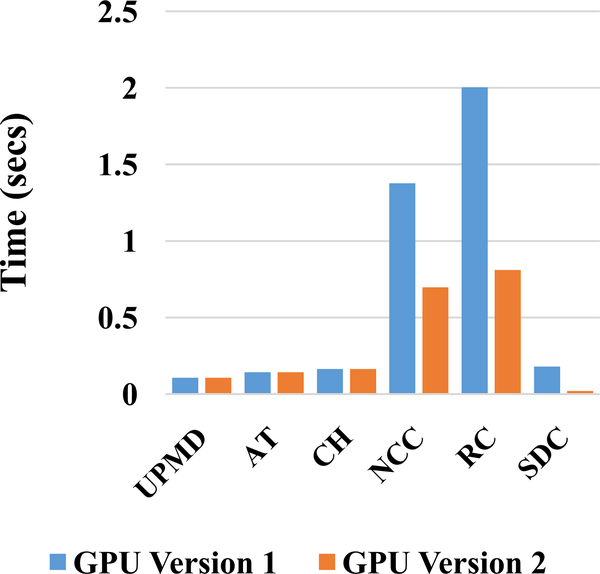
Speedup for level 3 of the SDC stage was just 4.67X, which was quite low indicating that the current configuration of the MLGPF algorithm utilizing 1024 grid points with 1024 threads was not optimal. SDC was not a notable part of the timing analysis in Fig. 1 however; it does become a notable component in GPU Version 1. The new bottlenecks for GPU Version 1 are the RC stage and CH+NCC stage. Hence, we further optimize RC, CH+NCC and SDC stages.

For both the RC and CH+NCC stages the NCC matrices sizes for level 1 through 3 respectively are 67×81 (5427), 41×59 (2419), 23×41 (943). These NCC matrices sizes are the optimal CUDA block size to use for the respective levels since if we use these block sizes, a unique thread can operate on each NCC matrix element. However, CUDA block sizes are limited to 1024 and sizes above these are not supported. Hence, the sizes used for level 1, level 2 and level 3 for both these stages were 32×32. 32×32 and 16×32 respectively and the same threads stepped through multiple NCC value calculation. This appears to be reasonable but is inefficient use of hardware. The problem requires understanding of the execution model on the GPU.

The execution model can be thought of as launching multiple CUDA blocks where each block has multiple threads. Execution of threads happens in the form of CUDA warps which are groups of 32 threads that run in lock-step fashion. If all 32 threads in each warp are not always performing useful calculations, it results in inefficient use of the GPU hardware. GPU Version 1 suffers from this issue and an example of this would be if we consider how warp 0 of level 1 in the RC or NCC stage would function. The threads ids in the form of (lateral, axial) or (X,Y) for warp 0 would be (0, 0), (1, 0), ….. (31,0). After doing the computation for the same offset as the thread ids these threads would step ahead to calculate for offsets (32,0), (33, 0), …. (63, 0). Next, they would step to (64, 0), (65, 0), …. (95, 0). The problem now is offsets from (67, 0) to (96, 0) do not exist and the threads working with these offsets are not doing useful work. This issue is called thread divergence. One solution is to simply change the block dimensions used. Thus, for level 1 since NCC size is 67×81, we launch CUDA blocks with size (67,15) using 1005 threads that still do not exceed 1024 threads. Therefore, the threads no longer iterate through the X or lateral dimension but only in the Y or axial dimension. Here the last warp is always divergent since the execution model will still use 1024 threads. However, all the other warps have non-divergent execution in the common case except for the last iteration which may have divergence for one warp computing the bottom rightmost offsets.

Further optimizations include use on chip shared memory and the texture cache which is a read only data cache. Shared memory can be thought of a cache managed by the programmer. Shared memory is especially useful with data reuse and we want this data to be loaded in shared memory before the threads start using it. Hence the threads typically load data in parallel then synchronize and start using the loaded data. This works great for the current image data block for NCC. However, since the search region is quite large for level 1 and level 2 the search region does not fit in the shared memory or it brings down occupancy of the implementation. Hence, we use texture cache for this which is very easy to use in compute capability 3.5 by simply giving compiler directives or intrinsics to mark the data to be loaded in texture cache. This can only be done if the data is read and never written to. For the RC stage although shared memory helps, there is not enough shared memory to load data from every neighboring NCC matrix into separate locations. Hence, the GPU implementation first loaded each neighbor synchronized threads, performed the computations, synchronized threads, overwrote the shared memory with a new neighbor, synchronized threads and then performed the next computation. Doing this with texture memory achieved the same effect without any synchronization overhead and hence provided better performance for the RC stage.

Next, we attempt to improve the performance of the MLGPF scheme. The motivation behind using 1024 threads was to use fewer numbers of iterations for the scheme to converge. This assumed that the 2D interpolation using windowed sinc function was computationally inexpensive. To test this assumption, we evaluate the difference between computational times with an implementation where the interpolator is removed. Of course, this produces incorrect results. The correct implementation takes 0.176 secs while after removing interpolation it only takes 0.004 secs. This shows that the windowed sinc function was the bottleneck in this scheme. Hence the next goal was to converge while performing fewer number of interpolations even if it meant increasing the number of iterations. Ignoring the relaxed shrinking factor, in every iteration we performed 1024 calculations to converge by a factor of 1/32 in each dimension. However, if we used just 64 threads and implemented shrinking of 1/8 in each iteration, we get a shrinking factor of 1/64 in two iterations while performing only 128 calculations. Hence, the number of threads used was changed to 64 instead of 1024. Nine iterations were needed instead of five iterations with 1024 threads. We also needed to use relaxed shrinking factors for the first four iterations. However, the scheme now takes 0.019 secs instead of 0.176 required with 1024 threads.

C. Comparison of GPU and CPU Performance

Lastly, we compare the quality of estimates generated by the CPU and final GPU implementations respectively. To achieve this we use the SNRe metric as reported in [25, 28] for the GPU and CPU implementation:

$$SN{R}_e=\frac{m_e}{s_e}$$

where m_e and s_e are the mean and standard deviation respectively of the resulting strain estimates. We also present strain maps from both implementations to provide a qualitative visualization. The SNRe study followed the same protocol used in McCormick et al. [25] with a uniform tissue-mimicking (TM) phantom undergoing precise deformation achieved using a motion table. Ten independent realizations were used to obtain statistically significant results.

Pointwise strain comparison on the TM phantom was also performed. To quantify the accuracy of the algorithm we report on the expected and observed strains by the CPU and GPU algorithms on the phantom. Finally, we report on the strain value difference in a human in vivo acquisition.

III. Results

Performance comparison results are reported for radiofrequency (RF) data acquired using a Siemens S2000 system (Siemens Ultrasound, Mountain View, CA), using an 18L6HD transducer operated at center frequency of 11.4 MHz. The dimensions of the acquired frames and the decimated sizes for different levels are presented in Table IV. Table V lists the number of data blocks that were required at different levels. No overlap between data blocks was used. As mentioned in [6], overlap is not used because guidance is already provided by higher levels for the final level and independent matching blocks are ideal for Bayesian regularization. Note that both CPU and GPU implementations are flexible for any frame size, up sampling ratios, decimation factors, search region ratios and desired amount of overlap between blocks. The configuration specified in Tables II through V is that used in our carotid plaque patient studies [3–5, 31–33]. GPU speedups and optimization can vary depending on the configuration and hence the configuration that was successfully used in our previous analysis on human subjects was optimized.

Table IV.

Frame Sizes with Siemens RF data, [Lateral, Axial]

Type	Frame Size
Read	[456,2076]
Up sampled	[912,4156]
Level 1	[456, 1384]
Level 2	[912, 2076]
Level 3	[912,4156]

Table V.

Number of blocks, [Lateral, Axial]

Level	Number of blocks
1	[14,24]
2	[37,44]
3	[45,114]

Table VI and VII show the effect of different optimizations for the CH+NCC and RC stage respectively. The second column presents the computational time for Version 1 which does not include these optimizations. In the third column we changed the CUDA block dimensions to 67×15, 41×24 and 23×41 for level 1 through 3 respectively and both stages completed faster. The shared memory and/or the texture cache configuration that worked best is shown in the last columns and is used in the final version.

Table VI.

Shared Memory and Texture Cache for NCC (time in seconds)

Levels	VI	Basic Optimizations to VI	Current Image in Shared Memory	All possible on Shared Memory	Texture memory For Next Image	Texture for Next Image in Level 1 and 2 and shared for level 3 Next Image
1	0.32	0.23	0.19	0.19**	0.16	0.16
2	0.52	0.38	0.32	0.33*	0.27	0.27
3	0 54	0.36	0.33	0.27	0.28	0.27

^*Theoretical occupancy is below 50% due to shared memory bottleneck

^**Next Image doesn't fit in shared memory

Table VII.

Shared Memory and Texture Cache for RC (time in seconds)

Levels	VI	Basic Optimizations to VI	Shared Memory	Texture Cache
1	0.46	0.39	0.36*	0.16
2	0.59	0.51	0.27	0.26
3	0.95	0.73	0.43	0.39

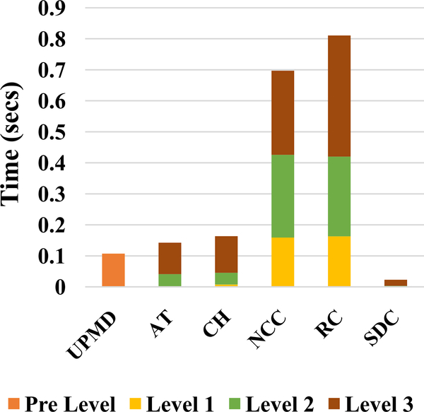
Computation time taken by both the GPU implementations to complete the different stages is presented in Fig. 3. Detailed GPU implementation timing analysis of the final version is presented in Fig. 4. The speedups for all levels and the different stages and net speedups are shown in Table VIII. Finally, the time taken by the different implementations and the associated speedup for a frame pair is shown in Table IX.

Fig. 3.

Timing comparison of GPU Version 1 and 2

Fig. 4.

Timing analysis for GPU Version 2

Table VIII.

Speed ups for Final GPU Version

Level	UPMD	AT	CH+ NCC	RC	SDC
1	NA	NA	75.54	287.96	216.41
2	NA	89.40	56.31	263.69	23.21
3	NA	73.78	35.47	270.58	37.185
Net	85.69	77.06	50.61	271.89	36.47

Table IX.

Application wide speed up and Time taken for a frame pair

	Time (secs)	Cumulative speed up
CPU	317.25	NA
GPU Version 1	3.91	81.13
GPU Version 2	1.88	168.75

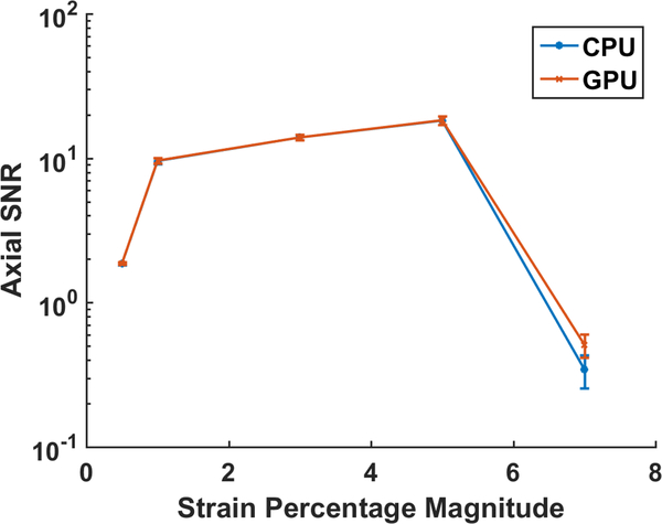
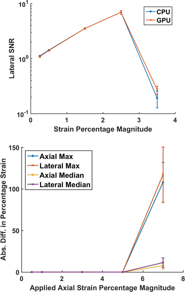
Quantitative comparison of the strain SNRe with the CPU and final GPU implementations are shown in Fig. 5 for a uniform TM phantom for 10 independent realizations. Note that the two implementations have very similar performance and the GPU version performs slightly better at increased deformation of 7% and 3.5% in the axial and lateral direction respectively.

Fig. 5.

Axial and Lateral SNR for the uniform phantom

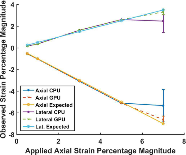
Figure 6 presents the median strain value obtained in the same uniformly elastic TM phantom. The expected strain is plotted with the estimated CPU and GPU strain. The average median value with error bars indicating the standard error is shown in Fig. 6. Note that there is excellent agreement between the CPU and GPU estimates with the expected strain upto 5 percent uniaxial deformation. However, when the uniaxial deformation is increased to 7 percent the CPU algorithm provides a worse performance when compared to the GPU also seen in the SNRe results in Fig. 5. To quantify differences between GPU and CPU implementations a pixel-to-pixel absolute difference of the corresponding strain maps were computed and the median and maximum absolute differences obtained shown in Fig. 7. Note that the absolute differences are nearly zero upto a 5% applied deformation but the CPU performs poorly for the 7% uniaxial deformation. In a similar manner the absolute difference in maximum strain observed for an in vivo plaque, was 6×10⁻⁴, 6×10⁻⁴ and 4×10⁻⁴ for accumulated axial, lateral and shear strain respectively between the CPU and GPU implementations.

Fig. 6.

Expected and observed strain in a uniformly elastic TM phantom

Fig. 7.

Pointwise absolute difference between CPU and GPU strain maps

As mentioned previously we use a 4-byte single precision floating point format for storing the up-sampled RF data for the GPU whereas the CPU used a 2-byte format. This leads to minor differences in values computed with the algorithm for low to moderate strains. However, as observed for the 7% axial strain case in Figs. 5–7 the GPU provides better estimation than the CPU.

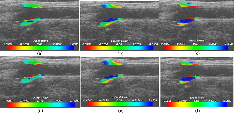
Finally, a qualitative comparison is presented in Fig. 8 on an in vivo acquisition on a human patient with carotid plaque in the longitudinal view. The two approaches identify similar areas in plaque with high strains.

Fig. 8.

Axial (a), lateral (b) and shear (c) strain for original CPU Implementation. In a similar manner (d), (e) and (f) represent the same strain tensor for GPU Version 2.

IV. Discussion And Conclusion

Note that the largest speedups were obtained for the regularization step in our algorithm. Bayesian regularization is a computationally intensive process with a high amount of data reuse leading to the high speedups. Data reuse is defined as same or contiguous data elements used by threads running in parallel. Algorithm with high data reuse have high speedups because it is typically more computationally expensive to fetch data. The GPU execution model enables performance of more computations with less fetches if there is good data reuse. NCC stage speedups are slightly lower as we go to higher stages, with smaller data block sizes and hence the amount of data reuse is less when compared to lower stages.

Many researchers have described implementations of NCC on GPU’s previously. Idzenga et al. [11] noted that approximately 90% of their computational time was spent performing NCC in their CPU implementation. In comparison, in our approach we spent 15.08% of our computational time on NCC, excluding the DU stage. Most of the time 77.35%, was spent on Bayesian regularization. The remaining 8% was spent on up-sampling, affine transformations and SDC using a 2D windowed sinc function for interpolation.

For NCC, after accounting for MATLAB to C/C++ transfer speedup, Idzenga et al. reported speedups of 67.33X for large cross correlation block sizes of 256×9 and speedup of 10.25X for smaller cross correlation block sizes of 16×9 using a NVIDIA K20 GPU. Peng et al. [16] also used NCC for threedimensional (3D) cross correlation estimation and reported speedups in the range of 120.21X to 107.69X for block sizes of 61×11×3 to 61×7×3, respectively. These speedups are comparable that reported in our paper of 75.54X to 35.47X for larger and smaller blocks respectively for NCC with the NVIDIA K40 GPU. In addition, literature reports also corroborate that smaller blocks have lower speedups because of lower data reuse.

However, only NCC computations have been previously reported with parallel computing implementations to the best of our knowledge. Thus implementing Bayesian regularization, 2D windowed sinc-interpolation which was used for up sampling, affine transformations and sub-sample estimation and the MLGPF scheme in parallel are unique contributions of this work. For SDC Peng et al. [16] used a matching cube and ellipsoid model for 3D coupled estimation and this took 27 ms with a NVIDIA K20 GPU. Our 2D windowed sincinterpolation based on the MLGPF scheme for sub-sample estimation took 19 ms for the final level. Both approaches are comparable in their computational times.

Overall the GPU implementation of displacement tracking provided a 168.75X speedup. However, this speedup considers a single-threaded CPU implementation. The DU stage which was used in the CPU does not provide any advantage and was removed in the CPU as well. After removing the DU stage from the CPU version we obtained a speedup of 151.53X with the GPU. Thus if we were to use a multi-threaded optimized CPU version it would need to run at least 152 threads in order to perform better than the GPU. If we assume that each core could run 2 threads without slowing down either of the threads, we would need a 76 core CPU. In fact, even with such a powerful CPU it would be unlikely that the CPU could match the performance because perfect thread to speedup scaling is never achieved due to intricate issues like false sharing [34], i.e. when two threads write into neighboring memory locations and cause a cache miss. There may also be memory bandwidth bottlenecks, load balancing, and core resource availability issues in such a CPU implementation.

Transferring the computation from CPU to GPU allowed for speedups in the displacement calculation. The strategies that helped in achieving this were, first identifying the computational bottlenecks and then working towards removing those with GPU implementation. This approach follows Amdahl [35] and is famously known as the Amdahl’s law in computer science. Secondly, we focused on minimizing data movement between the CPU and GPU as this is expensive. Finally, we explored GPU optimizations which focused on making the most efficient use of the GPU cores and memory bandwidth. The NVIDIA Visual Profiler (nvvp) was found to be a useful tool to implement all the above strategies.

GPU implementation makes it feasible for the algorithm to be clinically adopted since a cardiac cycle with 25 frames would now take about 50 secs whereas the original implementation would have taken 2.2 hours. Moreover, this opens up the opportunity for more computationally intensive approaches such as further up sampling of the data in the lateral dimension since ultrasound acquisitions have poor lateral resolution.

One should also note that there is scope for further speedup of the algorithm. With a speedup of NCC and RC stages as these are still our main bottlenecks as shown in Fig. 6. This is possible if we divide our data block calculation between multiple GPUs as we have enough data blocks for this to scale well. Lastly it is important to note that the Tesla k40c GPU used in this work is now three generations old as it belongs to the Kepler architecture (2012). Since then we have had Maxwell (2014), Pascal (2016) and Volta (expected) (2018) architectures. The newer generations will enable the GPU implementation to run even faster on these platforms.

Biography

Nirvedh H. Meshram, M.S. (S’16) received his B.Tech. in Electronics engineering from Veermata Jijabai Technological Institute (VJTI), Mumbai, India in 2014 and MS in electrical engineering in 2016 from the University of Wisconsin-Madison. Currently he is pursuing his PhD at University of Wisconsin-Madison in electrical engineering. His current research interests include elastography, ultrasound imaging, GPU computing and medical image analysis.

Tomy Varghese, Ph.D (S’92-M’95-SM’00) received the B.E. degree in Instrumentation Technology from the University of Mysore, India in 1988, and the M.S. and Ph.D in electrical engineering from the University of Kentucky, Lexington, KY in 1992 and 1995, respectively. From 1988 to 1990 he was employed as an Engineer in Wipro Information Technology Ltd. India. From 1995 to 2000, he was a post-doctoral research associate at the Ultrasonics laboratory, Department of Radiology, University of Texas Medical School, Houston, TX. He is currently a Professor in the Department of Medical Physics at the University of Wisconsin-Madison, Madison, WI. His current research interests include elastography, ultrasound imaging, quantitative ultrasound, detection and estimation theory, statistical pattern recognition and signal and image processing applications in medical imaging. Dr. Varghese is a fellow of the American Institute of Ultrasound in Medicine (AIUM), Senior member of the IEEE, and a member of the American Association of Physicists in Medicine (AAPM) and Eta Kappa Nu.

Appendix A

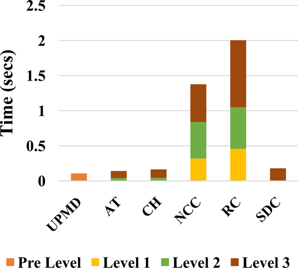
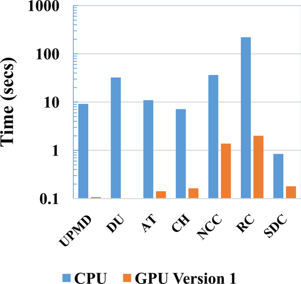
A timing analysis for GPU Version 1 is shown in Fig. A1. The NCC and RC stages become the main computational bottlenecks in GPU Version 1. To provide a clear comparison between GPU Version 1 and the CPU implementation a log plot comparing the timing is presented in Fig. A2. Log plot better represents the low computational times obtained with the GPU.

Fig. A1.

Timing Analysis for GPU Version 1

Fig. A2.

Comparison of GPU Version 1 to CPU on a log plot

References

- [1].Ophir J, Cespedes I, Ponnekanti H, Yazdi Y, and Li X, “Elastography: a quantitative method for imaging the elasticity of biological tissues,” Ultrasonic imaging,vol. 13, pp. 111–134, 1991. [DOI] [PubMed] [Google Scholar]
- [2].Regner DM, Hesley GK, Hangiandreou NJ, Morton MJ, Nordland MR, Meixner DD, et al. , “Breast Lesions: Evaluation with US Strain Imaging–Clinical Experience of Multiple Observers 1,” Radiology,vol. 238, pp. 425–437, 2006. [DOI] [PMC free article] [PubMed] [Google Scholar]
- [3].Dempsey RJ, Varghese T, Jackson DC, Wang X, Meshram NH, Mitchell CC, et al. , “Carotid atherosclerotic plaque instability and cognition determined by ultrasound-measured plaque strain in asymptomatic patients with significant stenosis,” Journal of Neurosurgery,pp. 1–9, 2017. [DOI] [PMC free article] [PubMed] [Google Scholar]
- [4].Wang X, Jackson DC, Mitchell CC, Varghese T, Wilbrand SM, Rocque BG, et al. , “Classification of Symptomatic and Asymptomatic Patients with and without Cognitive Decline Using Non-invasive Carotid Plaque Strain Indices as Biomarkers,” Ultrasound in medicine & biology,vol. 42, pp. 909–918, 2016. [DOI] [PMC free article] [PubMed] [Google Scholar]
- [5].Wang X, Jackson DC, Varghese T, Mitchell CC, Hermann BP, Kliewer MA, et al. , “Correlation of cognitive function with ultrasound strain indices in carotid plaque,” Ultrasound in medicine & biology,vol. 40, pp. 78–89, 2014. [DOI] [PMC free article] [PubMed] [Google Scholar]
- [6].McCormick M, Varghese T, Wang X, Mitchell C, Kliewer M, and Dempsey R, “Methods for robust in vivo strain estimation in the carotid artery,” Physics in Medicine & Biology,vol. 57, p. 7329, 2012. [DOI] [PMC free article] [PubMed] [Google Scholar]
- [7].Shi H, Mitchell CC, McCormick M, Kliewer MA, Dempsey RJ, and Varghese T, “Preliminary in vivo atherosclerotic carotid plaque characterization using the accumulated axial strain and relative lateral shift strain indices,” Physics in medicine and biology,vol. 53, p. 6377, 2008. [DOI] [PMC free article] [PubMed] [Google Scholar]
- [8].Hansen HH, de Borst GJ, Bots ML, Moll FL, Pasterkamp G, and de Korte CL, “Validation of noninvasive in vivo compound ultrasound strain imaging using histologic plaque vulnerability features,” Stroke,vol. 47, pp. 2770–2775, 2016. [DOI] [PubMed] [Google Scholar]
- [9].Huang C, Pan X, He Q, Huang M, Huang L, Zhao X, et al. , “Ultrasound-Based Carotid Elastography for Detection of Vulnerable Atherosclerotic Plaques Validated by Magnetic Resonance Imaging,” Ultrasound in medicine & biology,vol. 42, pp. 365–377, 2016. [DOI] [PubMed] [Google Scholar]
- [10].Shi H and Varghese T, “Two-dimensional multi-level strain estimation for discontinuous tissue,” Physics in medicine and biology,vol. 52, p. 389, 2007. [DOI] [PubMed] [Google Scholar]
- [11].Idzenga T, Gaburov E, Vermin W, Menssen J, and De Korte C, “Fast 2-D ultrasound strain imaging: the benefits of using a GPU,” IEEE transactions on ultrasonics, ferroelectrics, and frequency control,vol. 61, pp. 207–213, 2014. [DOI] [PubMed] [Google Scholar]
- [12].Verma P and Doyley MM, “Synthetic aperture elastography: A GPU based approach,” in Medical imaging 2014: Ultrasonic imaging and tomography, 2014, p. 90401A. [Google Scholar]
- [13].Rosenzweig S, Palmeri M, and Nightingale K, “GPU-based real-time small displacement estimation with ultrasound,” IEEE transactions on ultrasonics, ferroelectrics, and frequency control,vol. 58, 2011. [DOI] [PMC free article] [PubMed] [Google Scholar]
- [14].Loupas T, Powers J, and Gill RW, “An axial velocity estimator for ultrasound blood flow imaging, based on a full evaluation of the Doppler equation by means of a two-dimensional autocorrelation approach,” IEEE transactions on ultrasonics, ferroelectrics, and frequency control,vol. 42, pp. 672–688, 1995. [Google Scholar]
- [15].Yang X, Deka S, and Righetti R, “A hybrid CPU-GPGPU approach for real-time elastography,” IEEE transactions on ultrasonics, ferroelectrics, and frequency control,vol. 58, pp. 2631–2645, 2011. [DOI] [PubMed] [Google Scholar]
- [16].Peng B, Wang Y, Hall TJ, and Jiang J, “A GPU-Accelerated 3-D Coupled Subsample Estimation Algorithm for Volumetric Breast Strain Elastography,” IEEE Transactions on Ultrasonics, Ferroelectrics, and Frequency Control,vol. 64, pp. 694–705, 2017. [DOI] [PMC free article] [PubMed] [Google Scholar]
- [17].Lorensen WE and Cline HE, “Marching cubes: A high resolution 3D surface construction algorithm,” in ACM siggraph computer graphics, 1987, pp. 163–169. [Google Scholar]
- [18].Meunier J and Bertrand M, “Ultrasonic texture motion analysis: theory and simulation,” IEEE transactions on medical imaging,vol. 14, pp. 293–300, 1995. [DOI] [PubMed] [Google Scholar]
- [19].Jiang J and Hall TJ, “A coupled subsample displacement estimation method for ultrasound-based strain elastography,” Physics in medicine and biology,vol. 60, p. 8347, 2015. [DOI] [PMC free article] [PubMed] [Google Scholar]
- [20].Varghese T, Konofagou E, Ophir J, Alam S, and Bilgen M, “Direct strain estimation in elastography using spectral cross-correlation,” Ultrasound in medicine & biology,vol. 26, pp. 1525–1537, 2000. [DOI] [PubMed] [Google Scholar]
- [21].Chen L, Housden RJ, Treece GM, Gee AH, and Prager RW, “A hybrid displacement estimation method for ultrasonic elasticity imaging,” IEEE transactions on ultrasonics, ferroelectrics, and frequency control,vol. 57, pp. 866–882, 2010. [DOI] [PMC free article] [PubMed] [Google Scholar]
- [22].Chaturvedi P, Insana MF, and Hall TJ, “2-D companding for noise reduction in strain imaging,” IEEE transactions on ultrasonics, ferroelectrics, and frequency control,vol. 45, pp. 179–191, 1998. [DOI] [PubMed] [Google Scholar]
- [23].Varghese T and Ophir J, “Enhancement of echo-signal correlation in elastography using temporal stretching,” IEEE transactions on ultrasonics, ferroelectrics, and frequency control,vol. 44, pp. 173–180, 1997. [DOI] [PubMed] [Google Scholar]
- [24].McCormick M, Rubert N, and Varghese T, “Bayesian regularization applied to ultrasound strain imaging,” IEEE Transactions on Biomedical Engineering,vol. 58, pp. 1612–1620, 2011. [DOI] [PMC free article] [PubMed] [Google Scholar]
- [25].McCormick MM and Varghese T, “An approach to unbiased subsample interpolation for motion tracking,” Ultrasonic imaging,vol. 35, pp. 76–89, 2013. [DOI] [PMC free article] [PubMed] [Google Scholar]
- [26].Johnson HJ, McCormick M, and Ibanez L, “The ITK software guide,” Kitware, Inc.,2013. [Google Scholar]
- [27].McCormick M, Varghese T, Wang X, Mitchell C, Kliewer M, and Dempsey R, “Methods for robust in vivo strain estimation in the carotid artery,” Physics in medicine and biology,vol. 57, p. 7329, 2012. [DOI] [PMC free article] [PubMed] [Google Scholar]
- [28].Céspedes I, Huang Y, Ophir J, and Spratt S, “Methods for estimation of subsample time delays of digitized echo signals,” Ultrasonic imaging,vol. 17, pp. 142–171, 1995. [DOI] [PubMed] [Google Scholar]
- [29].Meshram NH and Varghese T, “Fast multilevel Lagrangian carotid strain imaging with GPU computing,” in Ultrasonics Symposium (IUS), 2017 IEEE International, 2017, pp. 1–4. [Google Scholar]
- [30].Harris M, “Optimizing cuda,” SC07: High Performance Computing With CUDA,2007. [Google Scholar]
- [31].Wang X, Mitchell C, Varghese T, Jackson D, Rocque B, Hermann B, et al. , “Improved correlation of strain indices with cognitive dysfunction with inclusion of adventitial layer with carotid plaque,” Ultrasonic imaging,vol. 38, pp. 194–208, 2016. [DOI] [PMC free article] [PubMed] [Google Scholar]
- [32].Berman SE, Wang X, Mitchell CC, Kundu B, Jackson DC, Wilbrand SM, et al. , “The relationship between carotid artery plaque stability and white matter ischemic injury,” NeuroImage: Clinical,vol. 9, pp. 216–222, 2015. [DOI] [PMC free article] [PubMed] [Google Scholar]
- [33].Meshram N, Varghese T, Mitchell C, Jackson D, Wilbrand S, Hermann B, et al. , “Quantification of carotid artery plaque stability with multiple region of interest based ultrasound strain indices and relationship with cognition,” Physics in Medicine & Biology,vol. 62, p. 6341, 2017. [DOI] [PMC free article] [PubMed] [Google Scholar]
- [34].Torrellas J, Lam H, and Hennessy JL, “False sharing and spatial locality in multiprocessor caches,” IEEE Transactions on Computers,vol. 43, pp. 651–663, 1994. [Google Scholar]
- [35].Amdahl GM, “Validity of the single processor approach to achieving large scale computing capabilities,” in Proceedings of the April 18–20, 1967, spring joint computer conference, 1967, pp. 483–485. [Google Scholar]