

The gas phase of mesophyll conductance is affected by the 3D traits tortuosity, path lengthening, and airspace connectivity, in addition to porosity.
Abstract
The leaf intercellular airspace (IAS) is generally considered to have high conductance to CO2 diffusion relative to the liquid phase. While previous studies accounted for leaf-level variation in porosity and mesophyll thickness, they omitted 3D IAS traits that potentially influence IAS conductance (gIAS). Here, we reevaluated the standard equation for gIAS by incorporating tortuosity, lateral path lengthening, and IAS connectivity. We measured and spatially mapped these geometric IAS traits for 19 Bromeliaceae species with Crassulacean acid metabolism (CAM) or C3 photosynthetic pathways using x-ray microcomputed tomography imaging and a novel computational approach. We found substantial variation in porosity (0.04–0.73 m3 m−3), tortuosity (1.09–3.33 m2 m−2), lateral path lengthening (1.12–3.19 m m−1), and IAS connectivity (0.81–0.97 m2 m−2) across all bromeliad leaves. The revised gIAS model predicted significantly lower gIAS in CAM (0.01–0.19 mol m−2 s−1 bar−1) than in C3 (0.41–2.38 mol m−2 s−1 bar−1) plants due to a coordinated decline in these IAS traits. Our reevaluated equation also generally predicted lower gIAS values than the former one. Moreover, we observed high spatial heterogeneity in these IAS geometric traits throughout the mesophyll, especially within CAM leaves. Our data show that IAS traits that better capture the 3D complexity of leaves strongly influence gIAS and that the impact of the IAS on mesophyll conductance should be carefully considered with respect to leaf anatomy. We provide a simple function to estimate tortuosity and lateral path lengthening in the absence of access to imaging tools such as x-ray microcomputed tomography or other novel 3D image-processing techniques.
By volume, as little as 3% (Slaton and Smith, 2002) and up to 73% (this study) of the inside of a leaf is composed of air. Such a wide range of values results from the multiple roles that mesophyll cells play in leaf function, the degree of reticulation of the embedded vein network, and cell size and shape, all reflecting the various adaptations plants have made in colonizing nearly every terrestrial habitat on Earth. From an evolutionary perspective, the transition from oceans to land exposed plant tissues to air, which dramatically lowered the resistance for CO2 diffusion to chloroplasts by ∼10,000-fold. Therefore, the evolutionary development of the leaf intercellular airspace (IAS) is considered a key innovation to profit from that lowered diffusion resistance (Ligrone et al., 2012). Yet, terrestrial inhabitation also exposed leaves to the risk of desiccation. Plants presumably navigated this tradeoff by developing a complex spatial cellular arrangement in order to produce a more or less tortuous 3D IAS network that rapidly delivered CO2 to the chloroplasts while maintaining a humid environment inside the leaf to limit evaporative water loss. Perhaps it is unsurprising then that the IAS has long been recognized as almost ubiquitous among terrestrial plants (Sifton, 1945).
Leaves utilizing Crassulacean acid metabolism (CAM) exhibit a major contrast in their IAS properties to those engaging the C3 metabolic pathway for photosynthesis, and they frequently occupy the lower end of the IAS volume morphospace. In comparison with C3 leaves, CAM leaves tend to have larger cells that are more densely packed into a given leaf volume, which typically results in lower porosity (Nelson et al., 2005). The tendency of CAM plants toward a higher cell volume fraction (i.e. lower porosity) enables greater nighttime storage of CO2 as malic acid in vacuoles, which is then decarboxylated and released as CO2 when stomata are closed during the light period (Nelson and Sage, 2008). Consequently, CAM metabolism is generally observed in plants such as epiphytes and succulents, which inhabit water-limited environments (Males, 2016; Griffiths and Males, 2017). C3 plants, on the other hand, tend toward smaller cell sizes, which presumably facilitates greater mesophyll surface exposure to the IAS, allowing more efficient carbon fixation by Rubisco (Maxwell et al., 1997; Griffiths et al., 2008). Lower leaf porosity, more typically associated with CAM metabolism but observed in some C3 plants, lowers the conductance to gas diffusion in the airspace, most often through lower exposure of mesophyll cells to the IAS (Galmés et al., 2013; Sáez et al., 2017). Thus, CAM plants must maintain a tradeoff that maximizes vacuolar CO2 storage capacity via tight cell packing while avoiding excessive diffusional costs as the IAS simultaneously shrinks.
Despite its potential impact on mesophyll conductance, the IAS generally is thought to have relatively higher conductance to CO2 diffusion than the liquid pathways in the leaf. In this study, we first examined the theoretical assumptions within the standard equations used to estimate the effect of IAS geometry on mesophyll conductance. This was done in the context of CAM versus C3 anatomies, as they represent one of the strongest anatomical contrasts with respect to the IAS in the plant kingdom. Specifically, we considered three IAS traits that often are overlooked due to their inherently 3D derivation and difficulty of measurement: tortuosity, lateral path lengthening, and IAS connectivity. Then, we measured and spatially mapped each of these IAS traits, along with other previously measured anatomical traits, for 19 CAM and C3 Bromeliaceae leaves using x-ray microcomputed tomography (microCT) imaging and used a novel set of computational algorithms. In doing this, we aimed to more accurately bound the geometric effect of IAS geometry on mesophyll conductance and provide direction for future research on the IAS.
A porous media approximation typically is used to calculate the effect of IAS geometry on the conductance of gas diffusion within the mesophyll pore space (gIAS: Syvertsen et al., 1995; Niinemets and Reichstein, 2003; Tomás et al., 2013):
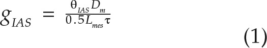 |
where θIAS is mesophyll porosity (m3 m−3), Dm is the diffusivity of CO2 in air (m2 s−1), 0.5Lmes is half mesophyll thickness (m), and τ is the tortuosity factor (m2 m−2). Due to its ease of measurement in two dimensions (2D), previous studies have focused almost exclusively on variation in the porosity term when quantifying the geometric effect of the IAS on mesophyll conductance. While no studies have calculated gIAS for CAM versus C3 species, the previously observed lower porosity values of CAM leaves (Nelson et al., 2005; Nelson and Sage, 2008) suggest a greater diffusive limitation in the IAS than for C3 plants, which corresponds with the very low mesophyll conductance values measured for the CAM species Kalanchoë daigremontiana (Maxwell et al., 1997; Griffiths et al., 2008).
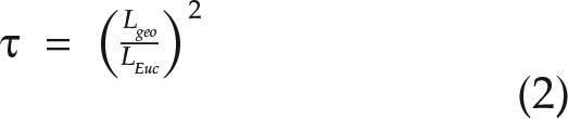
The complex interconnectivity of the mesophyll, in particular, should act to increase the path length of gaseous diffusion. Yet, due to its inherently 3D nature, IAS tortuosity has been measured only once, in leaves of Arabidopsis (Arabidopsis thaliana; Lehmeier et al., 2017). Moreover, little discussion of its definition and physical derivation exists in the plant literature. Tortuosity is defined as the ratio of the diffusive, or actual traveled, path length (i.e. the geodesic distance or Lgeo) to the straight, or unobstructed, path length (i.e. the Euclidean distance or LEuc; Gommes et al., 2009; see Fig. 1 for a schematic view of the distances measured and Fig. 2 for a contrasting view of Lgeo in two of the measured species). Given that the time, t, required for a molecule to diffuse over a given distance scales with the square of that distance, t ≈ L2/Dm, tortuosity has been shown to have a squared effect on diffusivity in porous media (Gommes et al., 2009). Consequently, the tortuosity factor τ (m2 m−2) can be defined as the square of the tortuosity:
Figure 1.

Diagram illustrating the derivation of the tortuosity factor (τ), lateral path lengthening (λ), and intercellular airspace (IAS) connectivity on a mesophyll-surface-area basis (κSA). A simplified cross section through a leaf is shown on the left with epidermal, stomatal, and parenchymal cells (green) and IAS (white). The vapor path length through the IAS, or geodesic distance (Lgeo; pink dashed line), can be decomposed into three components: lateral path length (Llat), epidermal path length (Lepi), and Euclidean path length (LEuc). A disconnected region of IAS and the associated mesophyll surface area is indicated by the solid orange outline.
Figure 2.

Volumetric rendering of leaf segments in the C3 leaf of Greigia sphacelata (left; δ13C = −31.3‰) and the CAM leaf of Aechmea penduliflora (right; δ13C = −15.1‰; δ13C values are from Crayn et al., 2015). Gray and white regions from the x-ray microCT image correspond with cell and IAS, respectively. White arrows indicate stomatal locations on the abaxial leaf surface. Diffusive path lengths (µm; Lgeo) within the IAS of each leaf are shown for the right half of each leaf.
 |
Based on theoretical values derived from the soil literature (Ball, 1981), the tortuosity factor for leaves is typically assumed to equal 1.55 (as used by Syvertsen et al. [1995] modeled using the approach of Ball [1981]) or 1.57 (Niinemets and Reichstein, 2003). However, the validity of this ubiquitous assumption in the plant literature and its variability in actual leaves are unknown. In other porous media (e.g. batteries, soils, and cement), a nonlinear negative relationship is typically observed between porosity and tortuosity (Boudreau, 1996; Moldrup et al., 2001; Shen and Chen, 2007; Zacharias et al., 2013). Hence, the low porosity of CAM leaves may be associated with high tortuosity, which would further decrease the diffusive conductance within the IAS.
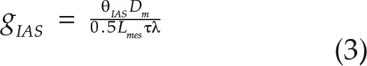
Lateral path lengthening is another inherently 3D property that is overlooked in the standard equations for calculating mesophyll conductance from IAS geometry. Lateral path lengthening results from CO2 entering the IAS through stomata that are distributed discretely across the epidermal surface (Parkhurst, 1994; Morison et al., 2005, 2007; Pieruschka et al., 2005, 2006, 2008; Morison and Lawson, 2007). As a result, CO2 must diffuse further to chloroplasts located along the mesophyll surface between two stomata than if the chloroplast is located directly above a stomate. Models of gIAS such as in Equation 1 are one dimensional along the leaf thickness axis and, as noted by Parkhurst (1994), assume that CO2 enters the IAS across the entire epidermis. We propose that lateral path lengthening, λ (m m−1), should be added to Equation 1 to account for this effect (Fig. 1):
 |
As cell packing becomes tighter, such as in CAM species, plants potentially risk disconnecting IAS channels completely, leading to isolated airspace volumes that only link to the atmosphere via a liquid pathway through the cell. Since CO2 diffuses ∼10,000 times slower in water than in air, IAS disconnection can dramatically reduce the CO2 supply rate to these isolated uptake sites, and their relative contribution to the total mesophyll surface area available for chloroplast inhabitation, and ultimately leaf-level photosynthetic capacity, should be low (Fig. 1). Except at coarse spatial scales (Long et al., 1989; Morison et al., 2007), IAS connectivity has not been measured in leaves; thus, its biological significance in CAM versus C3 species is unknown. Furthermore, IAS connectivity (κSA; m2 m−2), which we define as the fraction of the mesophyll surface area that is connected to the largest IAS pore (i.e. the largest connected airspace volume within a leaf sample; see Fig. 1 for a schematic representation), is not currently accounted for in the basic equations used to estimate conductance from mesophyll anatomy. Such a modification to the standard equation (Nobel, 2009) for mesophyll conductance would take the following form:
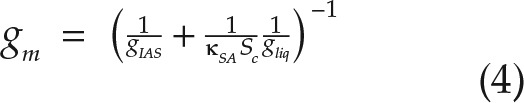 |
where Sc is the chloroplast surface area exposed to the IAS per square meter of leaf surface area and gliq is the liquid phase conductance, which can be subdivided into diffusive contributions from the cell wall, plasmalemma, cytosol, chloroplast envelope, and chloroplast stroma (Evans et al., 2009). Thus, in our formulation, IAS disconnection lowers mesophyll conductance by reducing the total mesophyll surface area available for diffusion.
Based on these theoretical considerations, it is clear that 3D IAS traits, beyond porosity, could contribute meaningfully to the gaseous phase of mesophyll conductance. Thus, we have measured these geometric traits from actual 3D IAS geometries in 19 Bromeliaceae species (Table 1) that capture a broad gradient of C3 and CAM types while constraining our study to a single family (see cross-sectional views in Fig. 3).
Table 1. Nineteen Bromeliaceae species investigated and the associated δ13C values from Crayn et al. (2015), CAM versus C3 classification based on a −20‰ threshold (Winter et al., 2015), and identifiers that correspond with images in Figure 3.
Definitions for plant habit are adapted from Males and Griffiths (2017).
| Species | δ13C | Habit | Growth Conditionsa | Identifier |
|---|---|---|---|---|
| ‰ | ||||
| CAM | ||||
| Tillandsia recurvata | −15.9 | Atmospheric epiphyte | GH | a |
| Tillandsia caulescens | −14.8 | Atmospheric epiphyteb | GH | b |
| Tillandsia usneoides | −14.4 | Atmospheric epiphyte | GH | c |
| Acanthostachys strobiliacea | −16.1 | Epiphyte | GH | d |
| Aechmea fulgens | −13.5 | Tank epiphyte | GH (UCD) | e |
| Hechtia marnier-lapostolleii | −11.9 | Terrestrial | Arid GH | f |
| Deuterochonia schreiteri | −11.4 | Terrestrial | Outdoor | g |
| Quesnelia marmorata | −14.0 | Terrestrial | GH | h |
| Bilbergia elegans | −16.6 | Tank epiphyte | GH (UCD) | i |
| Aechmea penduliflora | −15.2 | Tank epiphyte | GH | j |
| Hechtia caerulea. | −15.8 | Terrestrial | Arid GH | k |
| Aechmea fendleri | −11.1 | Tank epiphyte | GH (UCD) | l |
| C3 | ||||
| Ochagavia carnea | −21.5 | Terrestrial | Outdoor | m |
| Brocchinia hechtioides | −23.7 | Tank lithophyte | GH | n |
| Greigia sphacelata | −31.3 | Terrestrial | Outdoor | o |
| Pitcairnia tabuliformis | −30.2 | Terrestrial | GH | p |
| Guzmania zahnii | −24.0 | Tank epiphyte | GH | q |
| Nidularium innocenti | −33.3 | Tank epiphyte | GH (UCD) | r |
| Guzmania lingulata | −28.0 | Tank epiphyte | GH (UCD) | s |
GH stands for greenhouse, and all plants were grown at the University of California Botanical Garden (UCBG) except when specified (UCD, University of California Davis Botanical Conservatory). Growth conditions are described in “Materials and Methods.”
T. caulescens is probably a transition between tank and atmospheric epiphytes, as it is grown usually upward and has some small tanks.
Figure 3.

Segmented IAS (white), vascular and bundle sheath tissue (blue), and mesophyll tissue (green) for the 19 Bromeliaceae species examined. Letters correspond with the species outlined in Table 1.
RESULTS
Porosity, Cell Packing, and Mesophyll Surface Area
After controlling for phylogenetic relatedness, CAM and C3 bromeliads had significant differences in porosity (θIAS) at 0.1 ± 0.01 and 0.37 ± 0.07 m3 m−3, respectively (P < 0.01; Fig. 4). At the extreme ends of leaf porosity were the CAM species Tillandsia recurvata (0.04; Fig. 5a) and the C3 species Brocchinia hechtioides (0.73; Fig. 5n; Table 2). Conversely, mesophyll tissue accounted, on average, for 90% and 63% of total mesophyll volume, indicating a higher cell-packing density in CAM versus C3 bromeliads. CAM mesophyll cells tended to have a significantly larger diameter, Lcell, at 45 ± 3 µm than the cells in C3 species, at 21 ± 3 µm (P < 0.01; Fig. 4), with a minimum of 12 µm in Guzmania lingulata and a maximum of 70 µm in T. recurvata. While no statistical difference in mesophyll surface area exposure to the IAS on a leaf-surface-area basis (Sm) was observed between CAM and C3 species (P < 0.25; Fig. 4), the larger cells, lower porosity, and higher cell-packing density in CAM species corresponded with lower mesophyll surface area exposure to the IAS on a mesophyll-volume basis (Ames/Vmes; P < 0.05; Fig. 4).
Figure 4.

Leaf anatomical trait values for the 19 Bromeliaceae species studied. For C3 (blue; δ13C < −20‰; n = 7) and CAM (gray; δ13C > −20‰; n = 12) bromeliads (see Table 1 for a full species list), mesophyll thickness (Lmes; µm), mesophyll surface area per leaf area (Sm; m2 m−2), average cell diameter (Lcell; µm), mesophyll surface area exposed to the IAS per mesophyll volume (Ames/Vmes; µm2 µm−3), IAS porosity (θIAS; m3 m−3), IAS tortuosity (τleaf; m m−1), lateral path lengthening (λleaf; m m−1), and IAS connectivity on a mesophyll-surface-area basis (κSA; m2 m−2) are shown. Asterisks in the top left corner of the plots indicate significant differences (P < 0.05) between CAM and C3 bromeliads based on a phylogenetic paired Student’s t test.
Figure 5.

Average cross-sectional porosity (θIAS) for the 19 Bromeliaceae species examined in 3D collapsed into a 2D plane. Letters correspond with the species outlined in Table 1.
Table 2. For each species examined, leaf-level values of porosity (θIAS; m3 m−3), mesophyll thickness (Lmes; µm), tortuosity factor (τleaf; m2 m−2), lateral path lengthening (λleaf; m m−1), IAS connectivity (κSA; m2 m−2), leaf averaged geodesic path length (Lgeo,leaf; µm), and IAS conductance (gIAS; mol m−2 s−1 bar−1) were calculated from Equation 6.
| Species | θIAS | Lmes | τleaf | λleaf | κSA | Lgeo,leaf | gIAS |
|---|---|---|---|---|---|---|---|
| CAM | |||||||
| Acanthostachys strobiliacea | 0.10 | 588 | 1.29 | 1.55 | 0.88 | 1,035 | 0.10 |
| Aechmea fendleri | 0.05 | 130 | 1.57 | 2.51 | 0.92 | 409 | 0.11 |
| Aechmea fulgens | 0.12 | 519 | 1.64 | 1.53 | 0.87 | 1,017 | 0.11 |
| Aechmea penduliflora | 0.08 | 364 | 1.65 | 1.35 | 0.79 | 631 | 0.12 |
| Bilbergia elegans | 0.15 | 474 | 1.37 | 1.49 | 0.81 | 827 | 0.19 |
| Deuterochonia schreiteri | 0.16 | 701 | 1.28 | 1.14 | 0.94 | 904 | 0.19 |
| Hechtia caerulea | 0.08 | 374 | 1.32 | 1.30 | 0.86 | 559 | 0.16 |
| Hechtia marnier-lapostolleii | 0.20 | 652 | 1.42 | 1.64 | 0.91 | 1,274 | 0.16 |
| Quesnelia marmorata | 0.09 | 487 | 1.76 | 1.47 | 0.89 | 950 | 0.08 |
| Tillandsia caulescens | 0.04 | 540 | 2.20 | 3.19 | 0.92 | 2,555 | 0.01 |
| Tillandsia recurvata | 0.10 | 707 | 1.26 | 1.70 | 0.89 | 1,349 | 0.08 |
| Tillandsia usneoides | 0.04 | 591 | 3.33 | 2.52 | 0.90 | 2,718 | 0.01 |
| C3 | |||||||
| Brocchinia hechtioides | 0.73 | 340 | 1.09 | 1.12 | 0.97 | 398 | 2.17 |
| Greigia sphacelata | 0.38 | 396 | 1.14 | 1.41 | 0.92 | 596 | 0.73 |
| Guzmania lingulata | 0.40 | 127 | 1.12 | 1.46 | 0.90 | 196 | 2.38 |
| Guzmania zahnii | 0.37 | 168 | 1.13 | 1.90 | 0.94 | 339 | 1.28 |
| Nidularium innocentii | 0.30 | 152 | 1.23 | 1.33 | 0.94 | 224 | 1.48 |
| Ochagavia carnea | 0.19 | 335 | 1.23 | 1.42 | 0.95 | 528 | 0.41 |
| Pitcairnia tabuliformis | 0.20 | 223 | 1.17 | 1.30 | 0.92 | 314 | 0.74 |
Diffusive Path Lengthening
CAM bromeliads had significantly thicker mesophyll tissue at 511 ± 47 µm than C3 species at 249 ± 40 µm (Lmes; P < 0.01; Fig. 4). Aechmea fendleri, however, has exceptionally thin CAM leaves with a mesophyll thickness of 130 µm (Table 2). IAS tortuosity (τleaf) was on average 1.67 ± 0.17 m m−1 for CAM and 1.16 ± 0.02 m m−1 for C3 bromeliads (P < 0.01; Fig. 4), reaching extreme values of 1.09 and 3.33 in B. hechtioides (C3; Fig. 6n) and Tillandsia usneoides (CAM; Fig. 6c; Table 2). Lateral path lengthening (λleaf), while not significantly different between CAM and C3 species (P = 0.09), ranged broadly from 1.1 to 3.2 m m−1 (Fig. 4; Table 2) and was higher in species with a low stomatal density and/or long horizontal IAS channels like Guzmania zahnii (Fig. 7q) and Tillandsia caulescens (Fig. 7b). CAM bromeliads had an average diffusive path length (leaf-level averaged Lgeo [Lgeo,leaf]) of 1,186 ± 211 µm, whereas C3 species averaged 371 ± 56 µm (P < 0.01; Table 2; see Fig. 2 for a 3D rendering of Lgeo throughout the airspace of a C3 and a CAM species). Thus, thicker mesophyll tissue was associated with high tortuosity and long lateral path lengths that amplify the average diffusive path length.
Figure 6.

Average cross-sectional tortuosity factor (τleaf) for the 19 Bromeliaceae species examined in 3D collapsed into a 2D plane. Letters correspond with the species outlined in Table 1.
Figure 7.

Average cross-sectional lateral path lengthening (λleaf) for the 19 Bromeliaceae species examined in 3D collapsed into a 2D plane. Letters correspond with the species outlined in Table 1.
IAS Connectivity
C3 bromeliads had a significantly higher fraction of their mesophyll surface area connected to stomatal inlets, or κSA, at 0.94 ± 0.01 than CAM bromeliads at 0.88 ± 0.01 (P < 0.01; Fig. 4). Two CAM species, Aechmea penduliflora (Fig. 8j) and Bilbergia elegans (Fig. 8i), had the lowest values of κSA at 0.79 and 0.81, respectively, whereas the C3 species B. hechtioides (Fig. 8n) had the highest κSA of 0.97 (Table 2).
Figure 8.

Average cross-sectional likelihood of IAS disconnection (1 − κSA) for the 19 Bromeliaceae species examined in 3D collapsed into a 2D plane. Letters correspond with the species outlined in Table 1.
Coordination of Porosity with Tortuosity, Lateral Diffusivity, and IAS Connectivity
Porosity (θIAS) was nonlinearly and negatively related to tortuosity, with τleaf rising steeply as porosity became lower than ∼0.1 (Fig. 9;  , α = −0.18, P < 0.01, R2 = 0.55). Similarly, θIAS was nonlinearly and negatively related to the lateral diffusivity factor (Fig. 9;
  , α = −0.26, P < 0.01, R2 = 0.48). IAS connectivity on a mesophyll surface area basis (κSA), on the other hand, showed a nonlinear and positive relationship with θIAS (Fig. 9;
  , α = 0.05, P < 0.01, R2 = 0.19).
Figure 9.

Relationship between leaf-level porosity (θIAS; m3 m−3) and IAS tortuosity factor (τleaf; m2 m−2), lateral diffusivity factor (λleaf; m m−1), and IAS connectivity on the basis of mesophyll surface area (κSA; m2 m−2) for C3 (blue; δ13C < −20‰; n = 7) and CAM (gray; δ13C > −20‰; n = 12) bromeliads (see Table 1 for a full species list). Nonlinear regressions of the form  were used to relate θIAS to τleaf (α = −0.18, P < 0.01, R2 = 0.55), λleaf (α = −0.26, P < 0.01, R2 = 0.48), and κSA (α = 0.05, P < 0.01, R2 = 0.19).
IAS Conductance
Conductance of the intercellular airspace (gIAS) was calculated using the standard equation (Eq. 4) and our modified equation (Eq. 6). Using the standard equation (Eq. 4), which assumes a constant tortuosity factor of 1.57 and no lateral diffusivity, the average gIAS was 0.17 ± 0.02 mol m−2 s−1 bar−1 for CAM species and 1.36 ± 0.28 mol m−2 s−1 bar−1 for C3 (Fig. 10, open circles). After accounting for variation in τleaf and λleaf across species (Eq. 6) and for phylogenetic relatedness, CAM species had a significantly lower value of gIAS at 0.11 ± 0.02 mol m−2 s−1 bar−1 compared with C3 plants at 1.31 ± 0.28 mol m−2 s−1 bar−1 (P > 0.05; Fig. 10, closed circles). These changes corresponded with an average reduction in gIAS of 37% ± 25% (SD) for CAM species and 3.5% ± 16% for C3 species when compared with estimates using the assumed tortuosity factor of 1.57 (Fig. 10).
Figure 10.

IAS conductance (gIAS; mol m−2 s−1 bar−1) calculated using the standard equation (Eq. 4; open circles) and the modified equation (Eq. 6; closed circles) for C3 (blue; δ13C < −20‰; n = 7) and CAM (gray; δ13C > −20‰; n = 12) bromeliads. Percentage differences between the standard and modified equations are shown in parentheses to the right of the points. The approximate range of observed gm values from the literature as given by Flexas et al. (2008) is shown at the top. The presumed phylogenetic tree based on Givnish et al. (2011) is shown at far left.
Spatial Localization of Low IAS Conductivity
The leaves of CAM and C3 bromeliads varied broadly in their spatial distribution of porosity, tortuosity, lateral diffusivity, and intercellular airspace connectivity (Figs. 5–8). With the exception of the leaves of Ochagavia carnea, those of all C3 plants tended to have a large central IAS pore that became less porous radially toward the veins and epidermal surfaces (Fig. 5). While the leaves of some CAM plants, such as Aechmea fulgens and Deuterochonia schreiteri, had one or a few central air channels, the IAS tended to be smaller and more homogenous, also becoming less porous toward the veins and epidermal surfaces (Fig. 5). In both CAM and C3 leaves, high τleaf, λleaf, and κSA often were colocalized in low-porosity regions between the vein and the abaxial epidermis, suggesting a consistent pattern for low gIAS in these regions across bromeliads (Figs. 6–8). Several CAM species, such as A. penduliflora and Hechtia caerulea, had higher tortuosity and IAS disconnection surrounding the veins and in the abaxial regions of the mesophyll tissue (Figs. 6–8). Large regions of high-tortuosity tissue occurred in T. caulescens, T. usneoides, and Quesnelia marmorata (Fig. 6, b, c, and h).
DISCUSSION
CAM and C3 bromeliads have evolved distinct leaf geometries that correspond with their tendency to inhabit drier and wetter environments, respectively. While most of the plants sampled were grown in conservation greenhouses (Table 1), which might not reflect their natural growth environment and, therefore, might affect leaf anatomy and δ13C values, our results were similar to previous observations for Orchidaceae (Silvera et al., 2005, 2010), Asparagaceae (Heyduk et al., 2016), and Bromeliaceae (Maxwell, 2002; Pierce et al., 2002; Nelson et al., 2005) plants, with the values of some being measured on specimens from their native environment. On average, we found thicker leaves (Lmes) with larger cells (Lcell) in CAM versus C3 species (Fig. 4). When combined with significantly lower porosity (θIAS; Fig. 4), these traits led to greater cell packing (as in Nelson et al., 2005), giving rise to the succulent syndrome often associated with CAM species (Griffiths et al., 2008; Arakaki et al., 2011; Griffiths and Males, 2017). Hydraulically, high succulence allows for long-term water storage via chlorenchyma and/or hydrenchyma cells, which can buffer the effects of dehydration during prolonged periods without precipitation (Males, 2016). Larger cells with higher packing rates tend to reduce the total surface area that CAM plants can pack into their mesophyll volume (Ames/Vmes; Fig. 4), effectively lowering gas-exchange capacity by decreasing the liquid phase conductance at the leaf level (see Eq. 4; Nelson and Sage, 2008).
Theoretically, the distinct anatomical features of CAM plants (i.e. thick mesophyll and low porosity) should reduce mesophyll conductance (gm; see Lmes and θIAS in Eq. 1). Consistent with this prediction were the results of Griffiths et al. (2008), who measured a gm of 0.06 mol m−2 s−1 bar−1 in the CAM species K. daigremontiana, a value ∼40% lower than that measured for the related C3 species Kalanchoë pinnata. Isotopic measurements also point toward diffusional limitations within the mesophyll of K. daigremontiana (Griffiths et al., 2007). To the best of our knowledge, in addition to the studies by Griffiths et al. (2007, 2008 and the one by Maxwell et al. (1997) on K. daigremontiana, no other studies measured gm in other CAM species (Ripley et al. [2013] did measure it in some Aizoaceae plants, but those plants were largely performing C3 photosynthesis). More broadly across the plant kingdom, and based on this single observation, CAM plants are thought to possess among the lowest gm values, similar to or below those measured for evergreen gymnosperms and evergreen angiosperms (see refs. in Flexas et al. [2008] and the recent measurements reported by Veromann-Jürgenson et al. [2017]). Our estimation that, on average, for 12 CAM bromeliads, gIAS is 0.11 ± 0.02 mol m−2 s−1 bar−1, with extreme values of 0.01 and 0.19 mol m−2 s−1 bar−1 (Fig. 10), implies that the gm for these leaves is similar to or lower than the previously measured gm values for K. daigremontiana (0.06 mol m−2 s−1 bar−1; Maxwell et al., 1997; Griffiths et al., 2008) and at the lower end across the plant kingdom (Flexas et al., 2008; Fig. 10). Thus, the IAS likely plays a critical role in controlling gm within these CAM bromeliads and could represent about 50% of the total resistance to CO2 diffusion within the mesophyll (gIAS−1/gm−1 of K. daigremontiana = 0.11−1/0.06−1 = 0.54). The C3 bromeliads, on the other hand, had an average gIAS of 1.31 mol m−2 s−1 bar−1, with extreme minima and maxima of 0.41 and 2.38 mol m−2 s−1 bar−1 (Fig. 10), respectively, suggesting that gliq is the dominant constraint on gm for these species and as shown for multiple C3 species (Tomás et al., 2013; Tosens et al., 2016). However, for an accurate comparison of the respective contributions of gIAS and gliq to gm, one would need to measure cell anatomical features such as wall thickness, measurements that are lacking in our microCT data.
Across various plant taxa, the IAS is considered to have a relatively small effect on gm compared with liquid phase traits, particularly cell wall thickness (Flexas et al., 2008; Tomás et al., 2013; Carriquí et al., 2015). Typical estimations of gIAS, however, assume that only mesophyll thickness and porosity contribute to its variation; the tortuosity factor (τleaf) is generally held constant at 1.57, while potential effects of lateral path lengthening (λleaf) and IAS connectivity (κSA) are neglected because they were not empirically measurable until now. Here, we modified the standard equations to account for these additional IAS traits that are difficult to measure with traditional microscopy (Eqs. 1, 3, and 4). Incorporating variation in τleaf and λleaf in the estimation of gIAS had greater consequences for CAM bromeliads, with our new equation producing mean gIAS values 37% ± 25% lower (range from +6 to −82%) than one would calculate with previous equations. Our analysis of C3 leaf geometry, however, suggests that adding these new terms to the gIAS equation yields estimates only 3.5% ± 16% lower, with most species having estimates within 10% of those obtained using the old equation. Two extreme C3 deviations for gIAS were found, and these were caused by extreme λleaf values (+27%, B. hechtioides and −28%, G. zahnii; Fig. 10). This substantial variation among species highlights the importance of characterizing the 3D properties of the IAS when considering the relative contribution of gIAS to gm.
This study provides among the first measurements of leaf IAS tortuosity across a large leaf anatomical spectrum (for tortuosity measurement in Arabidopsis, see Lehmeier et al., 2017), as all other previous values were based on a simplified theoretical model from the soil literature (Ball, 1981). Our microCT measurements suggest that the standard assumption of 1.57 m2 m−2 for τleaf is an overestimate compared with our purely geometrical estimates for C3 (average of 1.16) and an underestimate for CAM bromeliads (average of 1.67; Fig. 4). Across the 19 species examined, we measured an approximately 3-fold range for τleaf (Fig. 4; Table 2), the value of which could be reasonably estimated as  (Fig. 9). Depending on the degree of variability in θIAS (Théroux-Rancourt et al., 2017), this relationship could be used to estimate τleaf based on 2D sections. Thus, τleaf tends to increase as porosity decreases, leading to a compounding effect on gIAS. In future studies, it would be interesting to investigate if the range of tortuosity values observed across CAM and C3 bromeliads is broadly representative for species throughout the plant kingdom.
Early theoretical work identified the potential importance of lateral diffusion for CO2 transport due to the discrete spacing of stomata (Parkhurst, 1977). Previous studies have since empirically demonstrated that lateral diffusion can contribute significantly to CO2 delivery within certain types of leaves by using spatially explicit gas-exchange and fluorescence measurements (Parkhurst, 1994;Morison et al., 2005, 2007; Pieruschka et al., 2005, 2006, 2008; Morison and Lawson, 2007). Despite these findings, the standard equation for estimating the IAS contribution to gm does not account for lateral diffusivity (Eq. 1). This omission necessarily underestimates the effect of lateral path lengthening (λleaf) for both CAM and C3 bromeliads and reflects the difficulty of making such measurements. We measured an average λleaf of 1.78 m m−1 for CAM and 1.42 m m−1 for C3 species and a nearly 3-fold range in variability (Fig. 4; Table 2). Similar to τleaf, a nonlinear and negative relationship exists between λleaf and θIAS (Fig. 9), suggesting a coordinated decline in gIAS due to multiple IAS traits simultaneously. Accounting for the effect of λleaf on gm might be especially important for species with low stomatal density and thin leaves. Nonangiosperms, such as lycophytes, ferns, conifers, and cycads, for example, tend to have relatively low stomatal densities (Franks and Beerling, 2009; Lammertsma et al., 2011), pointing toward an interesting avenue for future research.
Despite its potential impact on gm, IAS connectivity has rarely been studied in leaves. We are only aware of one investigation in which the upper and lower mesophyll of Zea mays leaves were shown to have low connectivity based on serial sectioning scanning electron microscopy (Long et al., 1989). In this study, we operationally define IAS connectivity (κSA) as the fraction of mesophyll surface area that is connected to the primary IAS pore. Presumably, CO2 diffusion due to pores (and associated surface area) disconnected from the primary IAS would be quite limited due to the presence of liquid cellular barriers. We measured an average κSA of 0.88 m2 m−2 for CAM and 0.94 m2 m−2 for C3 species, with that for leaves being as low as ∼0.8 m2 m−2 (Figs. 4 and 8; Table 2). The standard equations for estimating the IAS contribution to gm omit the effect of κSA and, consequently, based on our measurements, underestimate the effect of IAS disconnection on gm for both CAM and C3 bromeliads. However, it is important to note that the microCT scans used in this study have a voxel dimension of 0.64 µm, which results in a feature resolution of ∼1.9 μm. Since pore diameters below 1.9 µm likely exist in the IAS, our values of κSA are likely an underestimation. That said, pores around or below this diameter would be operating at the boundary of the Knudsen diffusion regime, in which the length of the mean free diffusive path is similar to the pore diameter (Leuning, 1983; Parkhurst, 1994), resulting in a constrictivity effect on diffusion. Moreover, as the ratio of mesophyll surface area to IAS volume increases with shrinking pore diameter, local reactive demand would effectively increase the resistance to vapor diffusion in favor of liquid diffusion. Future research using higher resolution imaging could examine if, when, and where IAS pores are truly disconnected via cell-to-cell barriers, along with the theoretical effects of reaction-diffusion systems operating within the Knudsen diffusion regime.
Vertical and lateral gradients in [CO2] are thought to exist throughout the leaf due to geometric and biochemical heterogeneity (Parkhurst and Mott, 1990; Pieruschka et al., 2005; Evans and Vogelmann, 2006; Earles et al., 2017). Our observations suggest substantial heterogeneity in gIAS throughout the mesophyll, as implicated by the spatial patterns of θIAS, τleaf, λleaf, and κSA (Figs. 5–8). Moreover, we find the tendency toward colocalization for each of these traits, often between the vein and the abaxial epidermis, which would amplify the reduction in gIAS within certain regions of the mesophyll. Depending on the distribution of reactive demand, this heterogeneity in gIAS could contribute to the generation of strong [CO2] gradients throughout the leaf. Such gradients may be particularly prevalent in CAM-type geometries during periods of Rubisco carboxylation, creating regions in which chloroplasts would have very limited access to CO2 unless CO2 is provided by malic acid decarboxylation. In this case, as the source of carbon would now originate from neighboring cells and not stomata, τleaf and λleaf values would be lowered, suggesting that CAM-type geometries could be optimized for the internal recycling of respiratory and decarboxylated CO2. It also would be interesting to understand if low-gIAS regions are effectively uninhabitable for chloroplasts due to low CO2 availability, a question that cannot be answered currently using our microCT data because chloroplasts are not visible. Moreover, whether such heterogeneity in gIAS corresponds with gradients in δ13C observed previously throughout the leaf (Robinson et al., 1993) is unknown.
In the absence of access to microCT or volumetric leaf anatomical data to measure τ and λ, we recommend estimating them together as a function of θIAS, assuming that the porosity value is representative of the leaf (Théroux-Rancourt et al., 2017). Multiplying the two functions of porosity presented previously gives  , or
, or  when fitting a power function to the product of τleaf and λleaf. Both functions are close to the assumption that tortuosity can be near θ−0.5 (Boudreau, 1996). Our data set covers a broad range of porosity values but is quite specific to certain leaf anatomy. Hence, θIAS−0.5 would be a reasonable replacement of τleaf and λleaf in Equation 3 and would be a better approach than using a literature value that might be unrepresentative of the studied leaf anatomy, especially at porosity values below 0.2 m3 m−3.
In conclusion, new methods such as microCT make IAS traits available and can extend our understanding of internal leaf geometry beyond porosity, which makes it possible to more accurately partition gm and gIAS. Based on our investigation of 19 CAM and C3 Bromeliaceae species, tortuosity, lateral path lengthening, and IAS connectivity are likely to have a significant impact on gIAS. Since these traits have largely not been measured in leaves, their broader influence on gIAS across the plant kingdom is unknown. Thus, we recommend that the potential impact of the IAS on gm be carefully reconsidered, and we have provided a suggestion on how to obtain a more representative tortuosity estimate from 2D cross sections based on a relationship to porosity. Imaging tools such as x-ray microCT and the 3D image-processing techniques employed in this study provide a platform for beginning to answer such questions.
MATERIALS AND METHODS
Plant Materials
We selected 19 Bromeliaceae species for analysis (Table 1), which capture a broad gradient of functional groups within both C3 and CAM types while constraining our study to a single family (see cross-sectional views in Fig. 3). Plants were classified as CAM or C3 based on the δ13C values described by Crayn et al. (2015); Table 1). While specifying an exact cutoff value is somewhat arbitrary, we defined CAM and C3 species as having δ13C values greater than −20‰ and less than −20‰, respectively, in accordance with Pierce et al. (2002) and Winter et al. (2015). Plant specimens were collected at UCBG from conservation and display greenhouses and from outdoor displays (Berkeley, CA) and at the UCD Botanical Conservatory greenhouse (for growth conditions, see Table 1). Both at UCBG and UCD, greenhouse plants were watered appropriately several times per week by their respective staff, and species grown in the arid greenhouse were watered once per week. Outdoor plants at UCBG received only rainfall during winter and were lightly watered once per week during the dry and rain-free months of summer, which might annually result in more water input than in their native habitats. For each species, several leaves from healthy plants were excised, immediately placed into a sealed plastic bag containing a damp paper towel, and stored in a dark insulated box. Leaves were then transported to the Lawrence Berkeley National Laboratory Advanced Light Source for x-ray microCT imaging at beamline 8.3.2 within 24 h of excision.
X-Ray MicroCT Imaging, Segmentation, and Classification
Samples were prepared for microCT imaging as described by Théroux-Rancourt et al. (2017). Before each scan (less than 30 min), one ∼1.5- to 2-mm-wide and ∼20-mm-long sample was excised near the first third of the leaf, starting from the apex of a fully developed leaf. They were then enclosed between two pieces of Kapton (polyimide) tape to prevent desiccation while allowing high x-ray transmittance. Subsequently, they were placed in a pipette tip, mounted in the sample holder, centered in the microCT x-ray beam, and scanned using the continuous tomography mode capturing 1,025 projection images at 21 keV, using a 10× objective lens, yielding a final pixel resolution of 0.64 µm. Each scan was completed in ∼15 min.
Image reconstruction was carried out using TomoPy, a Python-based framework for reconstructing tomographic data (Gürsoy et al., 2014). Each raw data set was reconstructed using both the gridrec (Dowd et al., 1999)and phase retrieval (Davis et al., 1995) reconstruction methods. Image stacks were rotated and aligned such that the veins were viewed in transverse section orthogonal to the epidermises. We then cropped the tissue to focus on a region of interest between the two major veins, such that the left and right image boundaries bisected two veins and the image was composed entirely of mesophyll. Sample regions where desiccation occasionally occurred during sample preparation were discarded. The final stacks contained ∼500 eight-bit grayscale images (downsampled from 32-bit images). Image processing was applied equally among scans using ImageJ software (Schneider et al., 2012).
The initial image segmentation and classification into IAS, mesophyll cell, vein, and background voxels also were performed as described by Théroux-Rancourt et al. (2017). For both the gridrec and phase-reconstructed images, the airspace was segmented first by visually and subjectively defining a range of pixel intensity threshold values between a minimum and a maximum grayscale value to optimize airspace classification while minimizing false classification (i.e. nonairspace pixels). After combining the binary image stacks from both reconstruction types, the mesophyll, veins, and background voxels were classified manually, which resulted in a composite image stack with cells, airspace, veins, and background voxels classified uniquely (Fig. 3).
Leaf-Trait Quantification from 3D Images
Mesophyll and Cell Dimensions
Cell diameter, Lcell (µm), was averaged for each species from measurements in ImageJ of 30 to 50 randomly selected cells in cross-section and paradermal slices. Mesophyll thickness, Lmes (µm), considered as the tissue excluding the epidermises and any hydrenchyma present, was averaged from over 10 cross sections and measured manually in ImageJ.
Mesophyll Porosity and Surface Area
As done by Théroux-Rancourt et al. (2017), the ImageJ plugin BoneJ Particle Analyzer function (Doube et al., 2010) with a resampling rate of 1 was used to quantify the IAS volume, VIAS (µm3), the total mesophyll volume (minus veins and epidermis), Vmes (µm3), and the mesophyll surface area exposed to the IAS, Ames (µm2). Mesophyll porosity, θIAS (m3 m−3), was then calculated as the IAS volume as a fraction of the total mesophyll volume. Cell packing was then simply defined as 1 – θIAS. Mesophyll surface area per mesophyll volume, Ames/Vmes (µm2 µm−3), was then calculated. Mesophyll surface area per projected leaf area, Sm (m2 m−2), was then calculated as the ratio Ames/Aleaf (m2 m−2), where Aleaf (m2) is the surface area of the leaf sample stack, defined as the image width multiplied by the stack depth (i.e. the area of the paradermal view).
Tortuosity, Lateral Diffusivity, and IAS Conductance
As in Equation 2, the tortuosity factor, τ (m2 m−2), was defined as the ratio of the diffusive path length within the IAS (i.e. the actual path from the stomate to a cell surface; geodesic distance [Lgeo]) to the straight path length in the absence of any physical obstacles to diffusion between the stomate and the cell surface (Euclidean distance, LEuc; Gommes et al., 2009; see Fig. 1 for a visual description of the different lengths measured). To calculate Lgeo and LEuc, we first generated a binary image of the stomatal inlets for each leaf. Then, we calculated two geodesic distance maps using the ImageJ plugin MorphoLibJ (Legland et al., 2016). The first map, Lgeo, quantified the shortest distance from the nearest stomatal inlet to all points along the mesophyll surface within the geometric bounds of the IAS (i.e. with cells causing obstructions that increase the path length). The second map, LEuc, quantified the Euclidean distance (i.e. the unobstructed distance, from the nearest stomatal inlet to all points along the mesophyll surface). In this way, we defined Lgeo and LEuc for all voxels along the mesophyll surface and simply calculated τ at these voxels using Equation 2 for the entire 3D image array. The leaf-level tortuosity, τleaf, was then calculated as the mean of τ, representing the average mesophyll surface voxel.
To calculate lateral path lengthening, λ (m m−1), we used the previously generated distance map, LEuc. Then, we created a second distance map, again using the ImageJ plugin MorphoLibJ (Legland et al., 2016), to quantify the shortest unobstructed straight-line distance between the lower epidermis and all points along the mesophyll surface, Lepi (Fig. 1). From these two distance maps, we calculated λ at all voxels along the mesophyll surface as:
By doing this, we quantified the surface-area weighted deviation from the standard 1D assumption that CO2 enters the IAS across the entire epidermis (Parkhurst, 1994). Leaf-level lateral path lengthening, λleaf, was then calculated as the mean of λ, representing the average mesophyll surface voxel.
Using leaf-level tortuosity and lateral diffusivity factors, we then calculated leaf-level IAS conductance as:
IAS Connectivity
We define IAS connectivity, κSA (m2 m−2), as the fraction of the mesophyll surface area that is connected to the largest IAS pore (i.e. the largest airspace volume [or connected voxels] within the leaf from the stomata to the palisade mesophyll). Based on the examination of our microCT data, the largest IAS pore is always connected to the stomata and, consequently, the atmosphere. Hence, any mesophyll surface area or volume that is not connected to the largest IAS pore is defined as disconnected. We apply the ImageJ plugin BoneJ Particle Analyzer function (Doube et al., 2010), which applies a three-pass nonrecursive approach to map voxel neighborhoods as in a graph and merges them, to quantify the volume and surface area of unique particles. We then quantify κSA as the surface area of the largest IAS particle divided by the sum of the surface area for all IAS particles. Since our microCT images have an isotropic voxel resolution of 0.64 µm, our technique would be less able to appropriately detect continuous IAS channels of a diameter less than 3 times the voxel resolution (1.9 µm diameter), which would lead to an apparent disconnection between two connecting larger volumes (addressed in “Discussion”).
2D Spatial Trait Maps
To examine the spatial distribution of porosity, the tortuosity factor, IAS connectivity, and the lateral diffusivity factor, we created 2D transverse projections for each trait. These projections show an average voxel value for each trait within a transverse leaf section. In the case of binary traits, like porosity and IAS connectivity, the 2D porosity projection defines the likelihood of IAS presence and connectivity, respectively. Thus, these projections have values ranging from 0 to 1. Importantly, the IAS connectivity likelihood value is conditional on IAS presence: so, a value of 0.9 indicates a 90% chance of IAS connectivity for a voxel stack that contains airspace. The tortuosity and lateral diffusivity factors, on the other hand, are average voxel values for each trait.
Statistical Analysis
Although many of the species used in this study have not been included in recent molecular phylogenetics studies of the Bromeliaceae, their taxonomy is well accepted. We used the R package pastis (Thomas et al., 2013) to generate a Nexus-formatted input for MrBayes (version 3.2.7; Ronquist et al., 2012), which used the species-level phylogeny from Givnish et al. (2011) as a constraint tree and the taxonomic affinities of species sequenced by Givnish et al. (2011) to place the species in this study into a well-resolved phylogeny. Bayesian analysis of this existing phylogeny was run for 50,000,000 generations with a 5,000,000-generation burn-in.
Phylogenetically controlled analyses were performed using the consensus tree generated by MrBayes. Phylogenetic Student’s t tests were performed using the phylANOVA function in the R package phytools (Revell, 2012). To assess evolutionary correlations between traits, Spearman rank correlations of phylogenetic independent contrasts (Felsenstein, 1985) were performed using the cor.table function in the R package picante (to improve normality, data were log transformed; Kembel et al., 2010). Because of the nonlinearity of the correlations between many traits, we used nonparametric Spearman rank correlations rather than parametric Pearson correlations between independent contrasts. To compare different methods for measuring the conductance of the intercellular airspace (gIAS), we used a phylogenetic paired Student’s t test (phyl.pairedttest) as implemented in the R package phytools. Nonlinear regressions between traits were performed using the nls library in the base R package.
Dive Curated Terms
The following phenotypic, genotypic, and functional terms are of significance to the work described in this paper:
Acknowledgments
We thank Ernesto Sandoval (UCD Botanical Conservatory) and Holly Forbes (UCBG) for the plant material collected. We also thank Sean McDowell (UCD) for assistance in data processing and Jamie Males for validating the growth habits of the studied Bromeliaceae plants. We thank John Evans and two anonymous reviewers for their helpful comments on the article.
Footnotes
G.T.-R. was supported by a Katherine Esau Postdoctoral Fellowship. A.B.R. was supported by the Yale Institute of Biospheric Studies. The Lawrence Berkeley National Laboratory Advanced Light Source is supported by the Director, Office of Science, Office of Basic Energy Sciences, of the U.S. Department of Energy under Contract No. DE-AC02-05CH11231.
Articles can be viewed without a subscription.
References
- Arakaki M, Christin PA, Nyffeler R, Lendel A, Eggli U, Ogburn RM, Spriggs E, Moore MJ, Edwards EJ (2011) Contemporaneous and recent radiations of the world’s major succulent plant lineages. Proc Natl Acad Sci USA 108: 8379–8384 [DOI] [PMC free article] [PubMed] [Google Scholar]
- Ball BC. (1981) Modelling of soil pores as tubes using gas permeabilities, gas diffusivities and water release. J Soil Sci 32: 465–481 [Google Scholar]
- Boudreau BP. (1996) The diffusive tortuosity of fine-grained unlithified sediments. Geochim Cosmochim Acta 60: 3139–3142 [Google Scholar]
- Carriquí M, Cabrera HM, Conesa MÀ, Coopman RE, Douthe C, Gago J, Gallé A, Galmés J, Ribas-Carbo M, Tomás M, et al. (2015) Diffusional limitations explain the lower photosynthetic capacity of ferns as compared with angiosperms in a common garden study. Plant Cell Environ 38: 448–460 [DOI] [PubMed] [Google Scholar]
- Crayn DM, Winter K, Schulte K, Smith JAC (2015) Photosynthetic pathways in Bromeliaceae: phylogenetic and ecological significance of CAM and C3 based on carbon isotope ratios for 1893 species. Bot J Linn Soc 178: 169–221 [Google Scholar]
- Davis TJ, Gao D, Gureyev TE, Stevenson AW, Wilkins SW (1995) Phase-contrast imaging of weakly absorbing materials using hard X-rays. Nature 373: 595–598 10.1038/373595a0 [DOI] [Google Scholar]
- Doube M, Kłosowski MM, Arganda-Carreras I, Cordelières FP, Dougherty RP, Jackson JS, Schmid B, Hutchinson JR, Shefelbine SJ (2010) BoneJ: free and extensible bone image analysis in ImageJ. Bone 47: 1076–1079 [DOI] [PMC free article] [PubMed] [Google Scholar]
- Dowd BA, Campbell GH, Marr RB, Nagarkar VV, Tipnis SV, Axe L, Siddons DP (1999) Developments in synchrotron x-ray computed microtomography at the National Synchrotron Light Source. In U Bonse, ed, SPIE's International Symposium on Optical Science, Engineering, and Instrumentation. SPIE, pp 224–236 10.1117/12.363725 [DOI]
- Earles JM, Théroux-Rancourt G, Gilbert ME, McElrone AJ, Brodersen C (2017) Excess diffuse light absorption in upper mesophyll limits CO2 drawdown and depresses photosynthesis. Plant Physiol 174: 1082–1096 [DOI] [PMC free article] [PubMed] [Google Scholar]
- Evans JR, Vogelmann TC (2006) Photosynthesis within isobilateral Eucalyptus pauciflora leaves. New Phytol 171: 771–782 [DOI] [PubMed] [Google Scholar]
- Evans JR, Kaldenhoff R, Genty B, Terashima I (2009) Resistances along the CO2 diffusion pathway inside leaves. J Exp Bot 60: 2235–2248 [DOI] [PubMed] [Google Scholar]
- Felsenstein J. (1985) Phylogenies and the comparative method. Am Nat 125: 1–15 [Google Scholar]
- Flexas J, Ribas-Carbó M, Diaz-Espejo A, Galmés J, Medrano H (2008) Mesophyll conductance to CO2: current knowledge and future prospects. Plant Cell Environ 31: 602–621 [DOI] [PubMed] [Google Scholar]
- Franks PJ, Beerling DJ (2009) Maximum leaf conductance driven by CO2 effects on stomatal size and density over geologic time. Proc Natl Acad Sci USA 106: 10343–10347 [DOI] [PMC free article] [PubMed] [Google Scholar]
- Galmés J, Ochogavía JM, Gago J, Roldán EJ, Cifre J, Conesa MÀ (2013) Leaf responses to drought stress in Mediterranean accessions of Solanum lycopersicum: anatomical adaptations in relation to gas exchange parameters. Plant Cell Environ 36: 920–935 [DOI] [PubMed] [Google Scholar]
- Givnish TJ, Barfuss MHJ, Van Ee B, Riina R, Schulte K, Horres R, Gonsiska PA, Jabaily RS, Crayn DM, Smith JAC, et al. (2011) Phylogeny, adaptive radiation, and historical biogeography in Bromeliaceae: insights from an eight-locus plastid phylogeny. Am J Bot 98: 872–895 [DOI] [PubMed] [Google Scholar]
- Gommes CJ, Bons AJ, Blacher S, Dunsmuir JH, Tsou AH (2009) Practical methods for measuring the tortuosity of porous materials from binary or gray tone tomographic reconstructions. AIChE J 55: 2000–2012 [Google Scholar]
- Griffiths H, Males J (2017) Succulent plants. Curr Biol 27: R890–R896 [DOI] [PubMed] [Google Scholar]
- Griffiths H, Cousins AB, Badger MR, von Caemmerer S (2007) Discrimination in the dark: resolving the interplay between metabolic and physical constraints to phosphoenolpyruvate carboxylase activity during the Crassulacean acid metabolism cycle. Plant Physiol 143: 1055–1067 [DOI] [PMC free article] [PubMed] [Google Scholar]
- Griffiths H, Robe WE, Girnus J, Maxwell K (2008) Leaf succulence determines the interplay between carboxylase systems and light use during Crassulacean acid metabolism in Kalanchöe species. J Exp Bot 59: 1851–1861 [DOI] [PubMed] [Google Scholar]
- Gürsoy D, De Carlo F, Xiao X, Jacobsen C (2014) TomoPy: a framework for the analysis of synchrotron tomographic data. J Synchrotron Radiat 21: 1188–1193 10.1107/S1600577514013939 [DOI] [PMC free article] [PubMed] [Google Scholar]
- Heyduk K, McKain MR, Lalani F, Leebens-Mack J (2016) Evolution of a CAM anatomy predates the origins of Crassulacean acid metabolism in the Agavoideae (Asparagaceae). Mol Phylogenet Evol 105: 102–113 [DOI] [PubMed] [Google Scholar]
- Kembel SW, Cowan PD, Helmus MR, Cornwell WK, Morlon H, Ackerly DD, Blomberg SP, Webb CO (2010) Picante: R tools for integrating phylogenies and ecology. Bioinformatics 26: 1463–1464 [DOI] [PubMed] [Google Scholar]
- Lammertsma EI, de Boer HJ, Dekker SC, Dilcher DL, Lotter AF, Wagner-Cremer F (2011) Global CO2 rise leads to reduced maximum stomatal conductance in Florida vegetation. Proc Natl Acad Sci USA 108: 4035–4040 [DOI] [PMC free article] [PubMed] [Google Scholar]
- Legland D, Arganda-Carreras I, Andrey P (2016) MorphoLibJ: integrated library and plugins for mathematical morphology with ImageJ. Bioinformatics 32: 3532–3534 [DOI] [PubMed] [Google Scholar]
- Lehmeier C, Pajor R, Lundgren MR, Mathers A, Sloan J, Bauch M, Mitchell A, Bellasio C, Green A, Bouyer D, et al. (2017) Cell density and airspace patterning in the leaf can be manipulated to increase leaf photosynthetic capacity. Plant J 92: 981–994 [DOI] [PMC free article] [PubMed] [Google Scholar]
- Leuning R. (1983) Transport of gases into leaves. Plant Cell Environ 6: 181–194 [Google Scholar]
- Ligrone R, Duckett JG, Renzaglia KS (2012) Major transitions in the evolution of early land plants: a bryological perspective. Ann Bot 109: 851–871 [DOI] [PMC free article] [PubMed] [Google Scholar]
- Long SP, Farage PK, Bolhár-Nordenkampf HR, Rohrhofer U (1989) Separating the contribution of the upper and lower mesophyll to photosynthesis in Zea mays L. leaves. Planta 177: 207–216 [DOI] [PubMed] [Google Scholar]
- Males J. (2016) Think tank: water relations of Bromeliaceae in their evolutionary context. Bot J Linn Soc 181: 415–440 [Google Scholar]
- Males J, Griffiths H (2017) Functional types in the Bromeliaceae: relationships with drought‐resistance traits and bioclimatic distributions. Funct Ecol 31: 1868–1880 [Google Scholar]
- Maxwell K. (2002) Resistance is useful: diurnal patterns of photosynthesis in C3 and Crassulacean acid metabolism epiphytic bromeliads. Funct Plant Biol 29: 679–687 [DOI] [PubMed] [Google Scholar]
- Maxwell K, von Caemmerer S, Evans JR (1997) Is a low internal conductance to CO2 diffusion a consequence of succulence in plants with Crassulacean acid metabolism? Aust J Agric Res 24: 777–786 [Google Scholar]
- Moldrup P, Olesen T, Komatsu T, Schjonning P, Rolston DE (2001) Tortuosity, diffusivity, and permeability in the soil liquid and gaseous phases. Soil Sci Soc Am J 65: 613–623 [Google Scholar]
- Morison JIL, Lawson T (2007) Does lateral gas diffusion in leaves matter? Plant Cell Environ 30: 1072–1085 [DOI] [PubMed] [Google Scholar]
- Morison JIL, Gallouët E, Lawson T, Cornic G, Herbin R, Baker NR (2005) Lateral diffusion of CO2 in leaves is not sufficient to support photosynthesis. Plant Physiol 139: 254–266 [DOI] [PMC free article] [PubMed] [Google Scholar]
- Morison JIL, Lawson T, Cornic G (2007) Lateral CO2 diffusion inside dicotyledonous leaves can be substantial: quantification in different light intensities. Plant Physiol 145: 680–690 [DOI] [PMC free article] [PubMed] [Google Scholar]
- Nelson EA, Sage RF (2008) Functional constraints of CAM leaf anatomy: tight cell packing is associated with increased CAM function across a gradient of CAM expression. J Exp Bot 59: 1841–1850 [DOI] [PubMed] [Google Scholar]
- Nelson EA, Sage TL, Sage RF (2005) Functional leaf anatomy of plants with Crassulacean acid metabolism. Funct Plant Biol 32: 409–419 [DOI] [PubMed] [Google Scholar]
- Niinemets Ü, Reichstein M (2003) Controls on the emission of plant volatiles through stomata: a sensitivity analysis. J Geophys Res 108: 4211 [Google Scholar]
- Nobel PS. (2009) Physicochemical and Environmental Plant Physiology. Elsevier, Oxford [Google Scholar]
- Parkhurst DF. (1977) A three-dimensional model for CO2 uptake by continuously distributed mesophyll in leaves. J Theor Biol 67: 471–488 [DOI] [PubMed] [Google Scholar]
- Parkhurst DF. (1994) Tansley Review No. 65. Diffusion of CO2 and other gases inside leaves. New Phytol 126: 449–479 [DOI] [PubMed] [Google Scholar]
- Parkhurst DF, Mott KA (1990) Intercellular diffusion limits to CO2 uptake in leaves: studies in air and helox. Plant Physiol 94: 1024–1032 [DOI] [PMC free article] [PubMed] [Google Scholar]
- Pierce S, Winter K, Griffiths H (2002) Carbon isotope ratio and the extent of daily CAM use by Bromeliaceae. New Phytol 156: 75–83 [Google Scholar]
- Pieruschka R, Schurr U, Jahnke S (2005) Lateral gas diffusion inside leaves. J Exp Bot 56: 857–864 [DOI] [PubMed] [Google Scholar]
- Pieruschka R, Schurr U, Jensen M, Wolff WF, Jahnke S (2006) Lateral diffusion of CO2 from shaded to illuminated leaf parts affects photosynthesis inside homobaric leaves. New Phytol 169: 779–787 [DOI] [PubMed] [Google Scholar]
- Pieruschka R, Chavarría-Krauser A, Cloos K, Scharr H, Schurr U, Jahnke S (2008) Photosynthesis can be enhanced by lateral CO2 diffusion inside leaves over distances of several millimeters. New Phytol 178: 335–347 [DOI] [PubMed] [Google Scholar]
- Revell LJ. (2012) phytools: an R package for phylogenetic comparative biology (and other things). Methods Ecol Evol 3: 217–223 [Google Scholar]
- Ripley BS, Abraham T, Klak C, Cramer MD (2013) How succulent leaves of Aizoaceae avoid mesophyll conductance limitations of photosynthesis and survive drought. J Exp Bot 64: 5485–5496 [DOI] [PMC free article] [PubMed] [Google Scholar]
- Robinson SA, Osmond CB, Giles L (1993) Interpretations of gradients in d13C value in thick photosynthesis tissues of plants with Crassulacean acid metabolism. Planta 190: 271–276 [Google Scholar]
- Ronquist F, Teslenko M, van der Mark P, Ayres DL, Darling A, Höhna S, Larget B, Liu L, Suchard MA, Huelsenbeck JP (2012) MrBayes 3.2: efficient Bayesian phylogenetic inference and model choice across a large model space. Syst Biol 61: 539–542 [DOI] [PMC free article] [PubMed] [Google Scholar]
- Sáez PL, Bravo LA, Cavieres LA, Vallejos V, Sanhueza C, Font-Carrascosa M, Gil-Pelegrín E, Javier Peguero-Pina J, Galmés J (2017) Photosynthetic limitations in two Antarctic vascular plants: importance of leaf anatomical traits and Rubisco kinetic parameters. J Exp Bot 68: 2871–2883 [DOI] [PMC free article] [PubMed] [Google Scholar]
- Schneider CA, Rasband WS, Eliceiri KW (2012) NIH Image to ImageJ: 25 years of image analysis. Nat Methods 9: 671–675 10.1038/nmeth.2089 [DOI] [PMC free article] [PubMed] [Google Scholar]
- Shen L, Chen Z (2007) Critical review of the impact of tortuosity on diffusion. Chem Eng Sci 62: 3748–3755 [Google Scholar]
- Sifton HB. (1945) Air-space tissue in plants. Bot Rev 11: 108–143 [Google Scholar]
- Silvera K, Santiago LS, Winter K (2005) Distribution of Crassulacean acid metabolism in orchids of Panama: evidence of selection for weak and strong modes. Funct Plant Biol 32: 397–407 [DOI] [PubMed] [Google Scholar]
- Silvera K, Neubig KM, Whitten WM, Williams NH, Winter K, Cushman JC (2010) Evolution along the Crassulacean acid metabolism continuum. Funct Plant Biol 37: 995–1010 [Google Scholar]
- Slaton MR, Smith WK (2002) Mesophyll architecture and cell exposure to intercellular air space in alpine, desert, and forest species. Int J Plant Sci 163: 937–948 [Google Scholar]
- Syvertsen JP, Lloyd J, McConchie C, Kriedemann PE, Farquhar GD (1995) On the relationship between leaf anatomy and CO2 diffusion through the mesophyll of hypostomatous leaves. Plant Cell Environ 18: 149–157 [Google Scholar]
- Théroux-Rancourt G, Earles JM, Gilbert ME, Zwieniecki MA, Boyce CK, McElrone AJ, Brodersen CR (2017) The bias of a two-dimensional view: comparing two-dimensional and three-dimensional mesophyll surface area estimates using noninvasive imaging. New Phytol 215: 1609–1622 [DOI] [PubMed] [Google Scholar]
- Thomas GH, Hartmann K, Jetz W, Joy JB, Mimoto A, Mooers AO (2013) PASTIS: an R package to facilitate phylogenetic assembly with soft taxonomic inferences. Methods Ecol Evol 4: 1011–1017 [Google Scholar]
- Tomás M, Flexas J, Copolovici L, Galmés J, Hallik L, Medrano H, Ribas-Carbó M, Tosens T, Vislap V, Niinemets Ü (2013) Importance of leaf anatomy in determining mesophyll diffusion conductance to CO2 across species: quantitative limitations and scaling up by models. J Exp Bot 64: 2269–2281 [DOI] [PMC free article] [PubMed] [Google Scholar]
- Tosens T, Nishida K, Gago J, Coopman RE, Cabrera HM, Carriquí M, Laanisto L, Morales L, Nadal M, Rojas R, et al. (2016) The photosynthetic capacity in 35 ferns and fern allies: mesophyll CO2 diffusion as a key trait. New Phytol 209: 1576–1590 [DOI] [PubMed] [Google Scholar]
- Veromann-Jürgenson LL, Tosens T, Laanisto L, Niinemets Ü (2017) Extremely thick cell walls and low mesophyll conductance: welcome to the world of ancient living! J Exp Bot 68: 1639–1653 [DOI] [PMC free article] [PubMed] [Google Scholar]
- Winter K, Holtum JAM, Smith JAC (2015) Crassulacean acid metabolism: a continuous or discrete trait? New Phytol 208: 73–78 [DOI] [PubMed] [Google Scholar]
- Zacharias NA, Nevers DR, Skelton C, Knackstedt K, Stephenson DE, Wheeler DR (2013) Direct measurements of effective ionic transport in porous Li-ion electrodes. J Electrochem Soc 160: A306–A311 [Google Scholar]