A sparse representation and dictionary learning based algorithm for image restoration in the presence of Rician noise

Abstract

Rician noise removal for Magnetic Resonance Imaging (MRI) is very important because the MRI has been widely used in various clinical applications and the associated Rician noise deteriorates the image quality and causes errors in interpreting the images. Great efforts have recently been devoted to develop the corresponding noise-removal algorithms, particularly the development based on the newly-established Total Variation (TV) theorem. However, all the TV-based algorithms depend mainly on the gradient information and have been shown to produce the so called “blocky” artifact, which also deteriorates the image quality and causes image interpretation errors. In order to avoid producing the artifact, this paper presents a new de-noising model based on sparse representation and dictionary learning. The Split Bregman Iteration strategy is employed to implement the model. Furthermore, an appropriate dictionary is designed by the use of the Kernel Singular Value Decomposition method, resulting in a new Rician noise removal algorithm. Compared with other de-noising algorithms, the presented new algorithm can achieve superior performance, in terms of quantitative measures of the Structural Similarity Index and Peak Signal to Noise Ratio, by a series of experiments using different images in the presence of Rician noise.

1. INTRODUCTION

The issue of image restoration in the presence of noise, (including either de-noising or de-noising plus de-blurring), is a basic and important topic in the field of image processing. Many de-noising algorithms have been proposed to deal with, for example, the Gaussian white noise [1][2], Poisson noise [3][4], multiplicative noise [5][6][7], and impulse noise [8][9]. As Magnetic Resonance Imaging (MRI) is being widely used in daily clinical applications, the associated Rician noise becomes a clinically-significant concern, because the noise deteriorates the image quality and causes errors in interpreting the images in the clinical applications. To relieve these concerns, our main goal here can be mathematically described as restoring the true (or desired) image u from the acquired image f, which is degraded by the Rician noise. For the particular Rician noise occurred in MRI, the degraded image f can be expressed as:

$$f=\sqrt{{(u+{\eta }_1)}^2+{\eta }_2^2}$$ (1)

where ${\eta }_1$ and ${\eta }_2$ represent independent Gaussian white noise.

Recently there have been many algorithms reported for removing the Rician noise, such as non-local mean filtering [10], wavelet packet [11], and wavelet domain filtering [12]. At the same time, other models or theories for Rician noise removal were presented, for example, the model proposed by Rudin, Osher and Fatemi [13], where the primal-dual algorithm [14] was employed to solve the model; and the maximum a posteriori (MAP) model [15], where the L² gradient-descent numerical method was used to solve the model. In the MAP model, the first item reflects the data fidelity under the image acquisition process condition and the second term considers the characteristics of the desired true image as much as possible. Unfortunately, these two items of the MAP model together render a non-convex cost function, resulting in a challenging task for solving the model or minimizing the cost function. To mitigate the challenge, Getreuer et al proposed a convex model [15] to approximate the MAP solution and solved the convex model by the Split Bregman Iteration (SBI) algorithm [16][17]. Although this approximated model is convex, its fidelity item is a piecewise function which is complicated and its mathematical properties are not very clear. To avoid the complication of the piecewise function, Chen et al [18] proposed a convex model to describe and remove the Rician noise, based on the newly-established Total Variation (TV) theorem.

Although the newly-established TV regularization strategy can preserve the nature of the edge very well, it will make flat areas spread along the edge direction and produce virtual edges inside a flat image area. This results in the so called blocky artifact. On the other hand, sparse is an important characteristic of natural images [19] and it has been applied successfully in the domain of image processing, such as image de-noising [20][21][22], image de-blurring [23], super resolution imaging [24][25][26][27], etc. Based on these two observations, a new regularization strategy for the Chen model [18] is proposed in this study. Using sparse representation, we avoid computing the gradient so the removal of Rician noise does not generate blocky artifacts. The SBI algorithm is employed to solve the new model or cost function. We update the associated dictionary in the sparse representation by the Kernel Singular Value Decomposition (K-SVD) algorithm [21] to find the most appropriate dictionary for image restoration. Compared with most of the TV-based Rician noise removing models, the effect of sparse feature representation used in this paper is much better. The experimental results show that our model can retain more edge details in the restored images.

The rest of this paper is organized as follows. Section 2 introduces the related works and our new model. Section 3 shows some experimental results. Conclusion is drawn in Section 4.

2. METHOD

2.1. Some relevant models

Getreuer et al. [15] propose a TV-based model based on the MAP framework. According to equation (1), f is a known degraded image and u is the original image. The probability distribution function of f, for Rician noise, is given by

$$P(f|u)=\frac{u}{{\sigma }^2}\exp (-\frac{u^2+f^2}{2{\sigma }^2})B_0(\frac{f\cdot u}{{\sigma }^2})$$ (2)

where $\sigma$ is the standard deviation of the noise, and $B_0$ is the modified Bessel function [28] of zero order $B_n(x)=\frac{1}{\pi }{\displaystyle {\int }_0^{\pi }{e}^{x\cos \theta }\cos (n\theta )d\theta }$. The MAP solution for the original image u is expressed as $\widehat{u}=\underset{u}{\arg max}P(u|f)$. By using the Bayes’ theorem, we obtain

$$\underset{u}{\arg max}P(u|f)\iff \underset{u}{\arg max}P(u)P(f|u)\iff \underset{u}{\arg min(-\log (P(u))-\log (P(f|u)))}$$ (3)

According to the Gibbs prior [5], we assume the prior $P(u)=\mathit{exp}(\gamma |\nabla u|dx)$, where $\gamma$ is a parameter and $\nabla$ is the gradient operator. Then, according to the Rician distribution (2), we can obtain

$$\underset{u}{\mathit{inf}}\left(\frac{1}{2{\sigma }^2}\underset{\mathrm{\Omega }}{\int }\left(u^2+f^2\right)dx-\underset{\mathrm{\Omega }}{\int }\log B_0\left(\frac{f·u}{{\sigma }^2}\right)dx+\mathrm{\gamma }\underset{\mathrm{\Omega }}{\int }|\nabla u|dx\right)$$ (4)

where $\mathrm{\Omega }$ is the image domain. Since the noisy image f is known, the model (4) can be written as

$$\underset{u}{\mathit{inf}}\left(\frac{1}{2{\sigma }^2}\underset{\mathrm{\Omega }}{\int }{u}^{2}dx-\underset{\mathrm{\Omega }}{\int }\log B_0\left(\frac{f·u}{{\sigma }^2}\right)dx+\mathrm{\gamma }\underset{\mathrm{\Omega }}{\int }|\nabla u|dx\right)$$ (5)

Chen et al. [18] add the penalty term $\frac{1}{\sigma }\underset{\Omega }{\int }{\left(\sqrt{u}-\sqrt{f}\right)}^{2}dx$ into the original model (5) and obtain a new model as follows

$$\underset{u}{\mathit{inf}}\left(\frac{1}{2{\sigma }^2}\underset{\mathrm{\Omega }}{\int }{u}^{2}dx-\underset{\mathrm{\Omega }}{\int }\log B_0\left(\frac{f·u}{{\sigma }^2}\right)dx+\frac{1}{\sigma }\underset{\mathrm{\Omega }}{\int }{\left(\sqrt{u}-\sqrt{f}\right)}^{2}dx+\mathrm{\gamma }\underset{\mathrm{\Omega }}{\int }|\nabla u|dx\right)$$ (6)

This model is solved by primal-dual algorithm [14]. In the rest of the paper, we refer to this as Chen’s model for simplicity.

2.2. The new model based on sparse representation and dictionary learning

2.2.1. The de-noising model

Assume $I\in R^N$ is an image (N represents the size of image, it also can be seen as a number of total pixels in the image if the image matrix piles up by column) and $I_i\in R^{N_i}$is one of the image patches extracted from the image I with size N_i. Using an over-complete dictionary matrix $D\in R^{N\times N_i}$, every image patch can find an appropriate sparse vector ${\alpha }_i\in R^{N_i}$ such that $I_i\approx D{\alpha }_i$. The entire image can also be represented by the set of $\left\{{\alpha }_i\right\}$and the sparse coefficients $\alpha$ obtained through all sparse vectors. We change the regularization term of the model (6) and rewrite it as:

$$\underset{u,\alpha }{min}\left(\frac{1}{2{\sigma }^2}{\Vert u\Vert }_2^2-\log B_0\left(\frac{f·u}{{\sigma }^2}\right)+\frac{1}{\sigma }{\Vert \sqrt{u}-\sqrt{f}\Vert }_2^2+\mu {\Vert \alpha \Vert }_0\right),s.tu=D\alpha$$ (7)

where f, u, B₀, $\sigma$ and $\alpha$ were defined before, $\mu$ is a parameter, ||·||₀and ||·||₂ represent 0-norm and 2-norm separately. The SBI algorithm [16] is used to solve the problem (7). Equation (7) can be converted into an equivalent form as follows,

$$\underset{u,\alpha }{min}\left(G\left(u\right)+R\left(\alpha \right)\right),s.t.u-D\alpha =0$$ (8)

where $G\left(u\right)=\frac{1}{2{\sigma }^2}{\Vert u\Vert }_2^2-\log B_0\left(\frac{fu}{{\sigma }^2}\right)+\frac{1}{\sigma }{\Vert \sqrt{u}-\sqrt{f}\Vert }_2^2$ and $R\left(\alpha \right)=\mu {\Vert \alpha \Vert }_0$. According to the SBI algorithm, the problem (8) can be solved as

$${\alpha }^{k+1}=\underset{\alpha }{\mathit{argmin}}\left(R\left(\alpha \right)+\frac{\rho }{2}{\Vert D\alpha -u^k+y^k\Vert }_2^2\right)$$ (9)

$$u^{k+1}=\underset{u}{\mathit{argmin}}\left(G\left(u\right)+\frac{\rho }{2}{\Vert D{\alpha }^{k+1}-u+y^k\Vert }_2^2\right)$$ (10)

$$y^{k+1}=y^k-\rho \left(u^{k+1}-D{\alpha }^{k+1}\right)$$ (11)

where y is the related variable of the SBI algorithm, $\rho$ is a parameter and k is the number of iteration. We will describe the solution of variables $\alpha$ and u in detail below.

The $\alpha$ sub-problem

The problem (9) can be rewritten as

$${\alpha }^{k+1}=\underset{\alpha }{\mathit{argmin}}\left(\frac{\mu }{\rho }{\Vert \alpha \Vert }_0+\frac{1}{2}{\Vert D\alpha -r^k\Vert }_2^2\right)$$ (12)

where $r^k=u^k-y^k$, every image patch $r_j=R_{j}r$, $R_j$ is an operator that extracts the patch $r^k$ from r. From the view of image patch, the problem (12) can be changed to

$$\widehat{\alpha }=\underset{\mathrm{\alpha }}{\mathit{argmin}}\left({\displaystyle \sum }_j\frac{1}{2}{\Vert D{\alpha }_j-R_j{r}^k\Vert }_2^2+{\displaystyle \sum }_j\frac{{\mu }_j}{\rho }{\Vert {\alpha }_j\Vert }_0\right)$$ (13)

where ${\mathit{\alpha }}_{\mathit{j}}$ is a sparse vector and ${\mathit{\mu }}_{\mathit{j}}$ is a parameter. Sparse image coefficient $\widehat{\mathit{\alpha }}$ can be obtained by Equation (13) and the initial training dictionary D is a complete DCT dictionary. The problem (13) can be solved by the orthogonal matching pursuit (OMP) algorithm [29]. Figure 1 is the procedure of the new model based on sparse representation and dictionary learning.

Figure 1.

The procedure of the new model based on sparse representation and dictionary learning.

The $u$ sub-problem

The problem (10) can be converted to:

$$\underset{u,v}{\mathit{min}}\left(G\left(u\right)+F\left(v\right)\right),s.t.u-v=0$$ (14)

where $G\left(u\right)=\frac{1}{2{\sigma }^2}{\Vert u\Vert }_2^2-\log B_0\left(\frac{fu}{{\sigma }^2}\right)+\frac{1}{\sigma }{\Vert \sqrt{u}-\sqrt{f}\Vert }_2^2$, $F\left(v\right)=\frac{\rho }{2}{\Vert D{\alpha }^{k+1}-v+y^k\Vert }_2^2$. According to SBI algorithm, the problem (14) can be changed to

$$v^{k+1}=\underset{v}{\mathit{argmin}}\left(F\left(v\right)+\frac{\lambda }{2}{\Vert u^k-v-b^k\Vert }_2^2\right)$$ (15)

$$u^{k+1}=\underset{u}{\mathit{argmin}}\left(G\left(u\right)+\frac{\lambda }{2}{\Vert u-v^{k+1}-b^k\Vert }_2^2\right)$$ (16)

$$b^{k+1}=b^k-\lambda \left(u^{k+1}-v^{k+1}\right)$$ (17)

where b is the related variable of the SBI algorithm and $\lambda$ is a parameter.

Solution of variable v

It can be seen from equation (15), solution of the variable v contains sparse coefficient $\alpha$, and then we can convert this problem into a sparse representation for each patch,

$$v^{k+1}=\underset{v}{\mathit{argmin}}\left({\displaystyle \sum }_j\frac{\rho }{2}{\Vert D{\alpha }_j^{k+1}-R_{j}v+y_j^k\Vert }_2^2+\frac{\lambda }{2}{\Vert u^k-v-b^k\Vert }_2^2\right)$$ (18)

The problem (18) is a convex problem and it can be solved as follows,

$$v^{k+1}={\left(\lambda E+\rho {\displaystyle \sum }_j{R}_j^T{R}_j\right)}^{-1}\left(\lambda \left(u^k-b^k\right)+\rho {\displaystyle \sum }_j{R}_j^T(D{\alpha }_j^{k+1}+y_j^k)\right)$$ (19)

where E is identity matrix and T means transpose.

Solution of variable u

The derivative equation of objective function (15) has a unique solution because the objective function is convex. Therefore, we can use the Newton’s method [7][15] to solve the derivative equation.

2.2.2. The model of de-noising plus de-blurring

The Rician noise removal model has been described in the past subsection. Now we will try to deal with the de-noising plus de-blurring problem by the new model. The two kinds of blur models we consider in this paper are Gaussian blur and motion blur. Meanwhile, images are also degraded by Rician noise. Some visual effects are shown in Fig. 2.

Figure 2.

MRI brain image with blur and noise. (a) original image; (b) Gaussian blur; (c) Motion blur; (d) Rician noise only; (e) Guassian blur plus Rician noise; (f) Motion blur plus Rician noise.

With both the system blur and the presence of Rician noise, the degraded image f can be expressed as

$$f=\sqrt{{(Au+{\eta }_1)}^2+{\eta }_2^2}$$ (20)

where A is a known linear blurring operator or a matrix if the image seen as a matrix. Then, the following optimization problem should be solved in order to restore image.

$$\underset{u,\alpha }{min}\left(\frac{1}{2{\sigma }^2}{\Vert \mathit{Au}\Vert }_2^2-\log B_0\left(\frac{Au·f}{{\sigma }^2}\right)+\frac{1}{\sigma }{\Vert \sqrt{\mathit{Au}}-\sqrt{f}\Vert }_2^2+\mu {\Vert \alpha \Vert }_0\right),s.t.u-D\alpha =0$$ (21)

Equation (21) can be converted into an equivalent form,

$$\underset{z,u,\alpha }{min}\left(G\left(z\right)+R\left(\alpha \right)\right),s.t.u-D\alpha =0,Au-z=0$$ (22)

where $G\left(z\right)=\frac{1}{2{\sigma }^2}{\Vert z\Vert }_2^2-\log B_0\left(\frac{f·z}{{\sigma }^2}\right)+\frac{1}{\sigma }{\Vert \sqrt{z}-\sqrt{f}\Vert }_2^2$, $R\left(\alpha \right)=\mu {\Vert \alpha \Vert }_0$, z is a variable and it is constrained by $Au$. Then, the problem (22) can be changed to

$$\underset{z,u,\alpha }{min}\left(\frac{1}{2{\sigma }^2}{\Vert z\Vert }_2^2-\log B_0\left(\frac{fz}{{\sigma }^2}\right)+\frac{1}{\sigma }{\Vert \sqrt{z}-\sqrt{f}\Vert }_2^2+\mu {\Vert \alpha \Vert }_0+\frac{{\rho }_1}{2}{\Vert D\alpha -u+y_1\Vert }_2^2+\frac{{\rho }_2}{2}{\Vert z-Au+y_2\Vert }_2^2\right)$$ (23)

where $y_1$ and $y_2$ are variables related to the SBI algorithm, ${\rho }_1$, ${\rho }_2$are two weighted parameters. The optimization problem (23) can be converted into the following sub-optimization problems

$${\alpha }^{k+1}=\underset{\alpha }{\mathit{argmin}}\left(R\left(\alpha \right)+\frac{{\rho }_1}{2}{\Vert D\alpha -u^k+y_1^k\Vert }_2^2\right)$$ (24)

$$z^{k+1}=\underset{z}{\mathit{argmin}}\left(G\left(z\right)+\frac{{\rho }_2}{2}{\Vert z-A{u}^k+y_2^k\Vert }_2^2\right)$$ (25)

$$u^{k+1}=\underset{u}{\mathit{argmin}}\left(\frac{{\rho }_1}{2}{\Vert D{\alpha }^{k+1}-u+y_1^k\Vert }_2^2+\frac{{\rho }_2}{2}{\Vert z^{k+1}-Au+y_2^k\Vert }_2^2\right)$$ (26)

$$y_1^{k+1}=y_1^k-{\rho }_1\left(u^{k+1}-D{\alpha }^{k+1}\right)$$ (27)

$$y_2^{k+1}=y_2^k-{\rho }_2\left(A{u}^{k+1}-z^{k+1}\right)$$ (28)

We will discuss the solution of the sub-problems one by one.

According to equation (24),

$${\alpha }^{k+1}=\underset{\alpha }{\mathit{argmin}}\left(\frac{\mu }{{\rho }_1}{\Vert \alpha \Vert }_0+\frac{1}{2}{\Vert D\alpha -r_1^k\Vert }_2^2\right)$$ (29)

where $r_1^k=u^k-y_1^k$, the problem (29) can be written as

$$\widehat{\alpha }=\underset{\alpha }{\mathit{argmin}}\left({\displaystyle \sum }_j\frac{1}{2}{\Vert D{\alpha }_j-R_j{r}_1^k\Vert }_2^2+{\displaystyle \sum }_j\frac{{\mu }_j}{{\rho }_1}{\Vert {\alpha }_j\Vert }_0\right)$$ (30)

This problem is similar to problem (13) and it also can be solved by OMP algorithm [29]. Then the initial training dictionary can be updated by K-SVD algorithm.

It is obvious that the objective function of problem (25) is strictly convex, we can use the same method as (16) to solve it. The sub-optimization problems of variables z and u can also be solved similarly as described in the previous section.

3. EXPERIMENTAL RESULTS

We use MATLAB 7.10 (R2010a) as the tool to carry out all algorithms on a PC with Windows 7 operating system. The parameter $\mu$ is manually selected as 1 in our algorithm for all experiments. De-noising performance is evaluated using the structural similarity index(SSIM) [30] and Peak Signal to Noise Ratio (PSNR) values in dB which is defined by

$$10\cdot {\log }_{10}(\frac{M^2}{\frac{1}{m\cdot n}{\displaystyle \sum _{i=1}^m{\displaystyle \sum _{j=1}^n{(u^{\prime }(i,j)-u(i,j))}^2}}})$$ (31)

where $u^{\prime }(x,y)$ denotes the restored image with respect to the original image $u(x,y)$, m and n are the width and height of image, $M=max(\underset{\begin{array}{l}1\le i\le m\\ 1\le j\le n\end{array}}{max}u(i,j),\underset{\begin{array}{l}1\le i\le m\\ 1\le j\le n\end{array}}{max}u\prime (i,j))$.

Figure 3 shows some slices of T1 and T2 MRI images obtained from [30]. All slices come from normal brain MRI images with slice thickness of 1 mm, no noise, and no intensity non-uniformity. There are 181 slices for one 3D MRI brain image. We chose some slices manually that contain more brain information for testing. The result of the new model will be compared with MAP model [15], Getreuer’s model [15] and Chen’s model [18]. Some visual effects of T2 weighted MRI images are shown in Fig. 2. Figure 4 shows the corresponding SSIM and PSNR values for the images in Fig. 2. Together these demonstrate that our model produces better results than the traditional methods on T2 weighed MRI images. The average time of MAP model, Getreuer’s model, Chen’s model and our model are 58.2896, 45.9461,60.7792 and 1774.2 seconds separately. Our model will spend more time due to the dictionary learning. At the same time, the cost also depends on the size of the image, the hardware and software of the computer. It can be sped up with a stronger computer and optimized algorithm.

Figure 3.

Some slices of MRI images with size 217×181.

Figure 4.

Experimental results for different slices. The 1^st, 2^nd, 3^rd rows are 78^th, 88^th, 98^th slice from the same 3D T2 weighted MRI image. The 1^st, 2^nd, 3^rd, 4^th, 5^th 6^th columns are original image, noisy image, the result of MAP model, Getreuer’s model, Chen’s model and our model separately.

The de-noised results of A T1 weighted MRI image slice and their corresponding SSIM and PSNR values under different models are shown in Table 1 and Fig. 6. The details of images obtained by our model are clearer than the results of other models. Notably, the blocky artifact that appears from the other models does not occur in the images generated by our model. This is more obvious for images with heavier noise levels. The SSIM and PSNR values in Fig. 6 also reflect this phenomenon. Figure 6 and Table 1 show that our model is superior to other models, not only in visual effects, but also in SSIM and PSNR values.

Table 1.

The results of images and SSIM, PSNR values of de-noised Brain MRI image under different models.

Figure 6.

SSIM and PSNR values of denoised Brain MRI image with different models.

We also test some natural images with Rician noise to further evaluate the effectiveness of our model. The size of the dictionary is 64×512 and the size of each image patch is 8×8 pixels. Experimental results indicate that our model is superior to the other three models on natural images with simulated Rician noise as well. The blocky artifact does not appear in the de-noised images from our model. This can be seen in Fig. 7, Fig. 8 and Fig. 9.

Figure 7.

Visual effects of different models in removing the Rician noise $\sigma =15$ of image “barbara”. (a) original image; (b) zoomed original image; (c) noisy image; (d) result of MAP model; (e) result of Getreuer’s model; (f) result of Chen’s model; (g) result of our model.

Figure 8.

Visual effects of different models in removing the Rician noise $\sigma =20$ of image “peppers”. (a) original image; (b) zoomed original image; (c) noisy image; (d) result of MAP model; (e) result of Getreuer’s model; (f) result of Chen’s model; (g) result of our model.

Figure 9.

Visual effects of different models in removing the Rician noise $\sigma =25$ of image “monarch”. (a) original image; (b) zoomed original image; (c) noisy image; (d) result of MAP model; (e) result of Getreuer’s model; (f) result of Chen’s model; (g) result of our model.

Figure 7 is the results of different models in removing the Rician noisy image “Barbara (512×512)” with $\sigma =15$. Figure 7(g) is the result of our model and the texture of it is clearer than other results. Figure 8 shows the de-noising results on image “peppers (256×256)” with Rician noise of standard deviation $\sigma =20$. The PSNR value of our model (seen in Fig. 8(g)) is higher than the results of the other three models. We test the de-noising method on “monarch (256×256)” with higher noise level of standard deviation $\sigma =25$ and the results are shown in Fig. 9. More PSNR values of experimental results are shown in Table 2. We also emphasize the results of our method and have marked them in bold color in the Table. The compared PSNR values can also be seen from Fig. 10 directly. It is obvious that the PSNR values of our results are higher than the other three models.

Table 2.

The result of PSNR(dB) values of denoised images under different models.

Image	Models	$\sigma =10$	$\sigma =15$	$\sigma =20$	$\sigma =25$
Barbara	Noisy	28.15	24.68	22.22	20.28
	MAP	30.55	26.72	25.46	24.59
	Getreuer’s	31.02	26.71	25.45	24.64
	Chen’s	31.09	28.02	25.77	24.95
	Ours	34.30	32.04	29.98	28.13
Peppers	Noisy	28.12	24.65	22.14	20.22
	MAP	33.21	30.19	29.09	27.02
	Getreuer’s	32.45	29.30	27.87	26.20
	Chen’s	33.21	30.77	29.18	27.40
	Ours	33.87	31.54	29.46	27.68
Monarch	Noisy	28.13	24.63	22.23	20.34
	MAP	33.83	30.04	28.94	26.95
	Getreuer’s	32.92	29.95	28.85	27.14
	Chen’s	32.99	30.49	28.93	27.23
	Ours	33.69	31.24	29.48	27.77
House	Noisy	28.15	24.59	22.15	20.23
	MAP	34.39	32.39	31.19	30.05
	Getreuer’s	34.33	32.26	30.98	29.99
	Chen’s	34.34	32.53	31.28	30.34
	Ours	35.85	34.05	32.60	31.12
Lena	Noisy	28.14	24.66	22.17	20.30
	MAP	34.19	31.87	30.62	29.55
	Getreuer’s	34.13	31.89	30.64	29.64
	Chen’s	34.17	32.27	30.94	29.79
	Ours	35.41	33.36	31.63	29.91
Boat	Noisy	28.15	24.65	22.17	20.24
	MAP	32.43	29.69	28.45	27.35
	Getreuer’s	32.42	29.74	28.44	27.55
	Chen’s	32.46	29.98	29.07	27.78
	Ours	33.42	31.37	29.54	27.92

Figure 10.

PSNR(dB) values of denoised image “Barbara”, “House” and “Lena” with different models.

Since we have demonstrated that our model outperforms the other three for both MRI and natural images, we test some natural images for de-blurring and de-noising where the effects are more readily visible. These images are tested with two kinds of blur models. One of them is Gaussian blur with the window size 9×9 and standard deviation is 1, the other is motion blur with the blur length 5 and the angle 30°. Meanwhile, after blurring, images are also degraded by Rician noise with $\sigma =20$. Figure 11 is the visual effects of different models in removing the Rician noise and Gaussian blur in image “boat (512×512)”. Fig. 12 shows the restored effects of “lena (512×512)” with Motion blur. Table 3 lists the corresponding PSNR values. We also emphasize the result of our method and have marked them in bold color in the Table. We note that in the presence of noise and blur, our model still performs better than the other three models tested.

Figure 11.

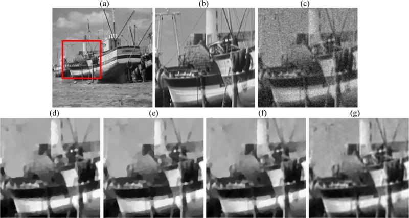
Visual effects of different models in removing the noise $\sigma =20$ and Gaussian blur in image “boat”. (a) original image; (b) zoomed original image; (c) noisy image; (d) result of MAP model; (e) result of Getreuer’s model; (f) result of Chen’s model; (g) result of our model.

Figure 12.

Visual effects of different models in removing the noise $\sigma =20$ and Motion blur in image “lena”. (a) original image; (b) zoomed original image; (c) noisy image; (d) result of MAP model; (e) result of Getreuer’s model; (f) result of Chen’s model; (g) result of our model.

Table 3.

The result of PSNR(dB) values of deblurring and denoised image under different models.

Image	Models	Gaussian Blur	Motion Blur
Boat	Degraded	21.40	21.12
	MAP	26.41	25.66
	Getreuer’s	26.25	25.86
	Chen’s	26.34	26.05
	Ours	26.52	26.05
Barbara	Degraded	23.55	20.12
	MAP	23.64	23.55
	Getreuer’s	23.57	23.50
	Chen’s	23.63	23.62
	Ours	23.78	23.71
Lena	Degraded	21.79	21.67
	MAP	29.20	28.61
	Getreuer’s	29.00	28.73
	Chen’s	29.08	28.84
	Ours	29.25	28.85

4. CONCLUSION

Image restoration is very important in the field of image processing. There are many types of noise and proposed methods to deal with them. For the particular Rician noise occurred in MRI, great efforts have been recently devoted to develop the corresponding noise-removal algorithms, most notably the development based on the newly-established Total Variation theorem. However, all the developed algorithms have produced the “blocky” artifacts, which deteriorate the image quality and causes image interpretation errors. On the other hand, sparse is an important characteristic of natural images and it has been applied successfully in the domain of image processing, such as image de-noising, image de-blurring, super resolution imaging, etc.

Based on these two observations, a new regularization strategy for Chen’s model is proposed in this study, based on sparse representation, to avoid gradient computing and therefore prevent the blocky artifact in removal of the Rician noise. The SBI algorithm is employed to solve the new model or cost function. We update the associated dictionary in the sparse representation by the K-SVD algorithm to find the most appropriate dictionary for image restoration. Compared with most of the TV-based Rician noise removing models, the effect of sparse feature representation used in this paper is much better. The experimental results show that our model can retain more edge details in the restored images.

Figure 5.

SSIM (top) and PSNR (bottom) values of denoised Brain MRI images corresponding to Fig. 3.

References

- 1.Buades A, Coll B, Morel J. A non-local algorithm for image denoising[J] IEEE Computer Society Conference on Computer Vision & Pattern Recognition. 2005;2(7):60–65. [Google Scholar]
- 2.Tai X, Borok S, Hahn J. Image denoising using TV-Stokes equation with an orientation-matching minimization[J] Scale Space and Variational Methods in Computer Vision. 2009;5567:490–501. [Google Scholar]
- 3.Le T, Chartrand R, Asaki T. A variational approach to reconstructing image corrupted by Poisson noise[J] Journal of Mathematical Imaging & Vision. 2007;27(3):257–263. [Google Scholar]
- 4.Zhang B, Fadili J, Starck J. Wavelets, ridgelets, and curvelets for Poisson noise removel[J] IEEE Transactions on Image Processing. 2008;17:1093–1108. doi: 10.1109/TIP.2008.924386. [DOI] [PubMed] [Google Scholar]
- 5.Aubert G, Aujol J. A variational approach to removing multiplicative noise[J] Siam Journal on Applied Mathematics. 2008;68(4):925–946. [Google Scholar]
- 6.Chen B, Cai J, Chen W, Li Y. A multiplicative noise removal approach based on partial differential equation model[J] Mathematical Problems in Engineering. 2012;2012:14. Article ID 242043. [Google Scholar]
- 7.Dong Y, Zeng T. A convex variational model for restoring blurred images with multiplicative noise[J] Siam Journal on Imaging Sciences. 2012;6(3):1598–1625. [Google Scholar]
- 8.Cai J, Chan R, Nikolova M. Two-phase approach for deblurring images corrupted by impluse plus Gaussian noise[J] Inverse Problems & Imaging. 2008;2(2):187–204. [Google Scholar]
- 9.Dong Y, Hintermuller M, Ner M. An efficient primal-dual method for L1-TV image restoration. Siam Journal on Imaging Sciences. 2009;27(4):1168–1189. [Google Scholar]
- 10.Wiest-Daessle N, Prima S, Coupe P, Morrissey S. Rician noise removal by non-local means filtering for low signal-to-noise ratio mri:Applications to DT-MRI[J] Medical image computing and computer-assisted intervention. 2008;5242(2):171–179. doi: 10.1007/978-3-540-85990-1_21. [DOI] [PMC free article] [PubMed] [Google Scholar]
- 11.Wood J, Johnson K. Wavelet packet denoising of magnetic resonance images: Importance of Rician noise[J] Magnetic Resonance in Medicine. 1999;41:631–635. doi: 10.1002/(sici)1522-2594(199903)41:3<631::aid-mrm29>3.0.co;2-q. [DOI] [PubMed] [Google Scholar]
- 12.Nowak R. Wavelet-based Rician noise removal for magnetic resonance imaging[J] IEEE Transactions on Image Processing. 1999;8:1408–1419. doi: 10.1109/83.791966. [DOI] [PubMed] [Google Scholar]
- 13.Rudin L, Osher S, Fatemi E. Nonlinear total variation based noise removal algorithms[J] Physica D Nonlinear Phenomena, pp. 1992:259–268. [Google Scholar]
- 14.Chambolle A, Pock T. A first-order primal-dual algorithm for convex problems with applications to image[J] Journal of Mathematical Imaging & Vision. 2011;40(1):120–145. [Google Scholar]
- 15.Getreuer P, Tong M, Vese L. A variational model for the restoration of mri images corrupted by blur and Rician noise[J] Lecture Notes in Computer Science. 2011;6938:686–698. [Google Scholar]
- 16.Goldstein T, Osher S. The split bregman algorithm for l1 regularized problems[J] Siam Journal on Imaging Sciences. 2009;2(2):323–343. [Google Scholar]
- 17.Zhao D, Zhang J, Zhao C, Gao W. Image compressive sensing recovery using adaptively learned sparsifying basis via l0 minimi-zation[J] Signal Processing. 2014;103:114–126. [Google Scholar]
- 18.Chen L, Zeng T. A convex variational model for restoring blurred images with large Rician noise[J] Journal of Mathematical Imaging & Vision. 2014;53(3):1598–1625. [Google Scholar]
- 19.Bruckstein A, Donoho D, Elad M. From sparse solutions of systems of equations to sparse modeling of signal and images[J] Siam Review. 2009;51(1):34–81. [Google Scholar]
- 20.Michael E, Michal A. Image denoising via sparse and redundant representation over learned dictionaries[J] IEEE Transactions on Image Processing. 2006;15(12):3736–3745. doi: 10.1109/tip.2006.881969. [DOI] [PubMed] [Google Scholar]
- 21.Michal A, Michael E, Alfred B. K-SVD: An algorithm for designing overcomplete dictionaries for sparse representation[J] IEEE Transactions on Signal Processing. 2006;54(11):4311–4322. [Google Scholar]
- 22.Zhang J, Zhao D, Gao W. Group-Based Sparse Representation for Image Restoration[J] IEEE Transactions on Image Processing. 2014;23(8):3336–3351. doi: 10.1109/TIP.2014.2323127. [DOI] [PubMed] [Google Scholar]
- 23.Shi G, Wu X, Dong W, Zhang L. Image deblurring and super-resolution by adaptive parse domain selection and adaptive regulariza-tion[J] IEEE Transactions on Image Processing. 2011;20(7):1838–1857. doi: 10.1109/TIP.2011.2108306. [DOI] [PubMed] [Google Scholar]
- 24.Marquina, Osher S. Image super-resolution by TV-regularization and bregman iteration[J] Journal of Scientific Computing. 2008;37:367–382. [Google Scholar]
- 25.Dong W, Zhang L, Shi G, Wu X. Image deblurring and super-resolution by adaptive sparse domain selection and adaptive regularization. IEEE Transactions on Image Processing. 2011;20(7):1838–1857. doi: 10.1109/TIP.2011.2108306. [DOI] [PubMed] [Google Scholar]
- 26.Xu J, Deng C, Liu X, et al. Image Super-resolution Based on Sparse Representation With Joint Constraints[C] 2014:381–385. [Google Scholar]
- 27.Yang J, Wright J, Huang TS, et al. Image super-resolution via sparse representation.[J] IEEE Transactions on Image Processing A Publication of the IEEE Signal Processing Society. 2010;19(11):2861–2873. doi: 10.1109/TIP.2010.2050625. [DOI] [PubMed] [Google Scholar]
- 28.Bowman F. Introduction to Bessel Functions. Dover Publicatuons; Mineoal: 2012. [Google Scholar]
- 29.Pati YC, Rezaiifar R, Krishnaprasad PS. Orthogonal matching pursuit: Recursive function approximation with applications to wavelet decomposition. Proceedings of 27th Asilomar Conference on Signals, Systems and Computers. 1993 [Google Scholar]
- 30.http://www.bic.mni.mcgill.ca/brainweb/