Application of multi-state models in cancer clinical trials

Abstract

Background/aims

The goal of this article is to illustrate the utility of multi-state models in cancer clinical trials. Our specific aims are to describe multi-state models and how they differ from standard survival methods, to illustrate how multi-state models can facilitate deeper understanding of the treatment effect on multiple paths along the disease process that patients could experience in cancer clinical trials, to explain the differences between multi-state models and time-dependent Cox models, and to briefly describe available software to conduct such analyses.

Methods

Data from 717 newly diagnosed acute myeloid leukemia patients who enrolled in the CALGB 10603 trial were used as an illustrative example. The current probability-in-state was estimated using the Aalen-Johansen estimator. The restricted mean time in state was calculated as the area under the probability-in-state curves. Cox-type regression was used to evaluate the effect of midostaurin on the various clinical paths. Simulation was conducted using a newly constructed shiny application. All analyses were performed using the R software.

Results

Multi state model analyses of CALGB 10603 suggested that the overall improvement in survival with midostaurin seen in the primary analysis possibly resulted from a higher complete remission rate in combination with a lower risk of relapse and of death after complete remission in patients treated with midostaurin. Simulation results, in a three-state illness-death without recovery model, demonstrate that multi-state models and time-dependent Cox models evaluate treatment effects from different framework.

Conclusion

Multi-state models allow detailed evaluation of treatment effects in complex clinical trial settings where patients can experience multiple paths between study enrollment and the final outcome. Multi-state models can be used as a complementary tool to standard survival analyses to provide deeper insights to the effects of treatment in trial settings with complex disease process.

Introduction

Time-to-event outcomes such as overall survival, progression-free-survival, or complete response are common clinical endpoints in oncology trials. These outcomes are often analyzed using common methods for survival or competing risks data such as the Kaplan-Meier estimator¹ or the cumulative incidence function² for descriptive analyses, or the log-rank test, the Cox proportional hazards regression,³ the Gray’s test, or the Fine-Gray model⁴ for inferences. These methods are appropriate and sufficient to understand treatment effects in settings where the disease process and the treatment options are simple or in situations where the only comparison of interest is the treatment effects on the final outcome regardless of intermediate events (as in intent-to-treat analyses). However, in trials where the combinations of disease process and treatment options are more complex or where intermediate events influence the trial outcomes, these standard methods alone do not provide a comprehensive picture of the effect of treatment on the intermediate events leading to the final outcome. Multi-state models are a powerful and flexible tool to explore treatment effects on intermediate events along multiple paths that patients can experience in these complex situations. One example of such situations was CALGB 10603, a randomized phase III clinical trial conducted by the Cancer and Leukemia Group B (CALGB), now part of the Alliance for Clinical Trials in Oncology. This trial evaluated the effect of midostaurin versus placebo, both in combination with daunorubicin and cytarabine, for treatment of newly diagnosed acute myeloid leukemia patients with fms-related tyrosine kinase 3 gene (commonly known as FLT3) mutation.⁵ The study treatment consisted of three phases: induction (1 to 2 cycles of 21 days), consolidation (4 cycles of 28 days), and maintenance (12 cycles of 28 days). Patients were allowed to receive blood and marrow transplantation per physician’s discretion at any time. This trial was an example of multiple paths along the treatment and disease process that patients could experience.

Figure 1 depicts a version of possible paths in this study. Specifically, all patients started at trial enrollment with newly diagnosed acute myeloid leukemia (denoted as Entry state). After enrollment, patients received the induction treatment prescribed to the arm to which they were randomized. Possible outcomes after induction included a first complete remission, a bone marrow transplant per physician’s discretion, or death. For patients who achieved first complete remission after induction, their possible future course included a transplant at physician’s discretion, disease relapse, or death. For patients who received transplant (patients are considered to be in complete remission immediately after transplant), their subsequent outcome was either relapse or death. Finally, for patients who had a relapse, they could receive a transplant if not have already received one earlier, a second transplant, or other salvage therapies to get to subsequent remissions. However, for simplicity of illustration, we only included transplant and death as possible subsequent states.

Figure 1.

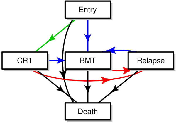
A multi-state model of CALGB 10603 trial

CR1: first complete remission, BMT: bone marrow transplant

Results of the primary analyses of CALGB 10603, using the log-rank tests and Cox proportional hazards regression, showed that the addition of midostaurin to daunorubicin and cytarabine was associated with an improvement in overall survival and event-free survival of newly diagnosed acute myeloid leukemia patients with fms-related tyrosine kinase 3 gene mutation.⁵ With the complex web of intermediate events in this trial, a natural question that might arise is where, specifically along the course of treatment, was midostaurin effective? Did it induce an earlier remission and/or did it prolong survival after the patient achieved remission? Was there any effect on relapse after remission? These questions may be answered one at a time by fitting several time-dependent Cox models or they can be answered simultaneously using multi-state models.

Despite its introduction by Aalen and Johansen in 1978⁶ and the fact that much has been written on this topic in the statistical literature,^6–16 multi-state models for censored observations have rarely been used in medical studies,^17,18 especially in oncology which often has a complex disease process that can benefit from multi-state analyses. Since much had been written about multi-state models from a theoretical perspective, this article focuses on their application. Specifically, the aims of this article are: a) to give a brief description of multi-state models, b) to illustrate the use of multi-state models using real data from a recent clinical trial (CALGB 10603), and c) to explain what multistate models can offer above and beyond common time-to-event analyses methods through a simulation study and describe available software to conduct such analyses. Our ultimate goal is to encourage the use of multi-state models in cancer clinical trials, to facilitate a better understanding of cancer disease process and its treatments. The benefits of multi-state models extend to many clinical research areas beyond cancer and should routinely be considered when analyzing time-to-event data.

Methods

Multi-state model

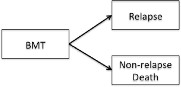
Multi-state modeling is a generalized framework to describe longitudinal events using the counting process.⁷ Each model consists of a set of states that one can occupy and the directions and states to which one can transition. A state in a multi-state model can be transient which means a subject can transition out of that state, or terminal which means, once a subject enters that state, departure is not possible. The simplest model consists of two states, for example a survival model with two states, Alive and Death (Figure 2a). The only possible transition in this model is from the initial state of being Alive (transient) to Death (terminal). Common examples of three-state models include the illness-death without recovery model (Figure 2b), which consists of two transient states, Health and Illness, and one terminal state, Death; or the competing risks model (Figure 2c) with one transient state, bone marrow transplant (denoted as BMT), and two terminal states, Relapse and Non-relapse Death. In the model in Figure 1, Entry, first complete remission (denoted as CR1), bone marrow transplant, and Relapse are all transient states while Death is, again, terminal.

Figure 2.

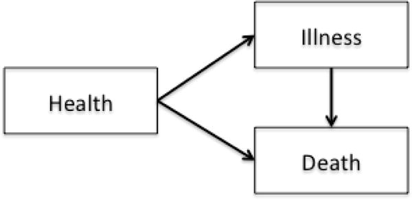
a. A two-state survival model

b. A three-state illness-death without recovery model

c. A competing-risk model

BMT: bone marrow transplant

Unlike standard survival methods where only terminal states are considered as outcomes, all states whether transient or terminal can be considered as outcomes in multi-state models, hence the effects of treatment and baseline factors on each transition can be evaluated. Multiple quantities can be obtained from multi-state models. The probability of being in a state can be estimated using the Aalen-Johansen estimator.⁶ A plot of probability-in-state is an insightful exploratory tool as illustrated in the CALGB 10603 dataset presented in the next section. The restricted mean time spent in each state can be estimated by calculating the area under the probability-in-state curves. Cox-type regression can also be conducted to evaluate treatment effects on all transitions simultaneously.

Results

Multi-state analysis of leukemia trial CALGB 10603 data

The purpose of this analysis is to illustrate the application of multi-state models and the complementary information that multi-state analysis can provide to help answer questions regarding the effect of treatment on various paths between study entry to intermediate events to death. Specific to this example, we evaluated the effect of midostaurin on first complete remission, relapse, and death. For clarity, the results presented in this section were based on a four-state model (Figure 3a). It is important to emphasize that the analyses and results presented here are intended for illustration of the method only and are not meant as recommendations for clinical practice or to replace the results presented in the primary trial manuscript.⁵

Figure 3.

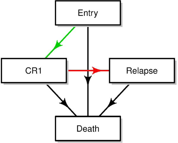
a. Multi-state model structure of CALGB 10603 data example

CR1: first complete remission

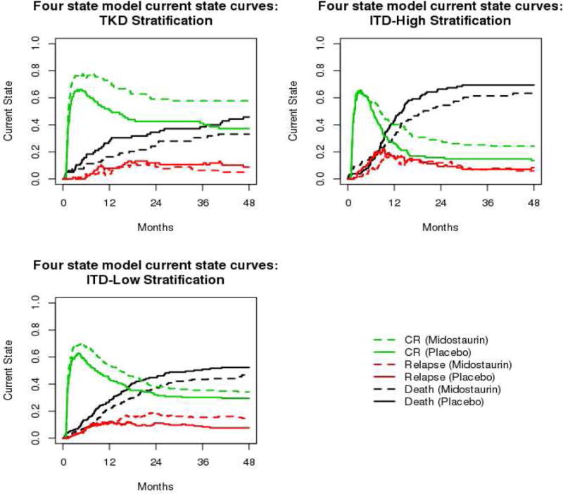
b. Plots of current state probabilities in leukemia data example

CR: complete remission, TKD: tyrosine kinase domain, ITD: internal tandem duplication

A total of 717 patients who were enrolled and randomized to midostaurin (n=360) or placebo (n=357) were included. Fms-related tyrosine kinase 3 gene status was a stratification factor with 162 (22%) patients with tyrosine kinase domain mutation versus 341 (48%) with low ratio internal tandem duplication versus 214 (30%) with high ratio internal tandem duplication. Among these patients, 504 (70%) achieved first complete remission during the course of treatment and 358 (50%) died by the end of the trial. Two hundred and thirty one (46% of 504) patients experienced relapse.

Figure 3b displays the current probability-in-state curves for all three states from time of study entry separately by fms-related tyrosine kinase 3 gene status. It showed that first complete remission (green curves in Figure 3b) occurred quickly. More than 60% of patients, across all strata, were in first complete remission within the first two months of study entry. First complete remission occurred more rapidly in the treatment group for patients with fms-related tyrosine kinase 3 gene tyrosine kinase domain mutation or with low ratio internal tandem duplication mutation. Across all fms-related tyrosine kinase 3 gene strata, midostaurin was associated with a higher likelihood of being in first complete remission. The most prominent effect was observed in the tyrosine kinase domain group. The likelihood of being in relapse (red curves in Figure 3b) is low across all strata. This likelihood appeared to be slightly higher for patients treated with midostaurin compared to placebo 12 months after study entry for the low ratio internal tandem duplication subgroup but appeared to be similar between arms for the other subgroups. Across all strata, mortality (black curves in Figure 3b) was consistently lower in the midostaurin arm. The highest likelihood of mortality was observed in patients with high ratio internal tandem duplication mutation. In summary, the current probability-in-state curves suggested that patients with tyrosine kinase domain mutation had the most favorable outcome (higher chance of being in first complete remission versus death or relapse) and patients with high ratio internal tandem duplication mutation had the worst outcome (higher likelihood of mortality compared first complete remission or relapse 12 months after study entry). Across all strata, midostaurin was associated with a higher likelihood of being in first complete remission and a lower likelihood of death. A slightly higher probability of being in relapse was observed in patients with low ratio internal tandem duplication mutation treated with midostaurin.

The mean time-in-state, restricted to 48 months from study entry, was also evaluated. Forty-eight months was used as the maximum time as this captures almost all events of interest. The “mean time-in-state” here refers to the amount of time, on average, that subjects spent in that state in the first 48 months after study entry. On average, patients treated with midostaurin spent more time in first complete remission than those in the placebo arm. This difference was observed in all strata, with mean time in first complete remission of 8.2 months, 3.3 months, and 4.9 months longer in the midostaurin arm compared to placebo for patients with tyrosine kinase domain, low ratio internal tandem duplication, and high ratio internal tandem duplication, respectively (rows 4–6 of Table 1). The mean time in relapse was 2.3 months longer in the midostaurin arm for patients in the low ratio internal tandem duplication subgroup compared to the placebo arm (row 8 of Table 1). In the 48 months after study entry, midostaurin was associated with an extension of 3–4 months of life across all strata (rows 10–12 of Table 1). These results are consistent with the conclusions drawn from the current probability-in-state curves and provide an alternative quantification of the effect of midostaurin.

Table 1.

Difference in mean time (months) in state restricted to the first 48 months from randomization between midostaurin and placebo arm

State	Fms-related tyrosine kinase 3 gene mutation strata	Difference	Standard error	P-valuea
Entry	Tyrosine kinase domain	−2.734	1.962	0.163
	Low Ratio Internal tandem duplication	−2.332	1.446	0.107
	High Ratio Internal tandem duplication	−0.829	1.730	0.632
First Complete Remission	Tyrosine kinase domain	8.229	3.292	0.012
	Low Ratio Internal tandem duplication	3.347	2.215	0.131
	High Ratio Internal tandem duplication	4.868	2.395	0.042
Relapse	Tyrosine kinase domain	−1.314	1.526	0.389
	Low Ratio Internal tandem duplication	2.322	1.208	0.055
	High Ratio Internal tandem duplication	−0.555	1.384	0.688
Death	Tyrosine kinase domain	−4.180	2.897	0.149
	Low Ratio Internal tandem duplication	−3.337	2.054	0.104
	High Ratio Internal tandem duplication	−3.484	2.533	0.169

^aP-value from Z-test using normal approximation

Cox-type regression was also conducted to evaluate effect of midostaurin on the transition rates. Results from the Cox-type regression (Table 2), stratified by fms-related tyrosine kinase 3 gene status, showed a slightly faster rate of first complete remission in the midostaurin arm (hazard ratio = 1.18, 95% confidence interval = (0.99–1.41), p value = 0.064) compared to the placebo arm and no difference in mortality rate without first complete remission (hazard ratio = 1.11, 95% confidence interval = (0.79–1.56), p = 0.546). After first complete remission, lower rate of relapse (hazard ratio = 0.77, 95% confidence interval = (0.59–1.00), p = 0.046) and lower rate of death (hazard ratio = 0.55, 95% CI = (0.32–0.96), p = 0.034) were observed in the midostaurin arm. The transition rates from relapse to death were similar between arm (hazard ratio = 0.97, 95% confidence interval = (0.71–1.32), p = 0.838). The overall improvement in survival with midostaurin seen in the primary analysis⁴ possibly resulted from a higher rate of first complete remission in combination with a lower relapse and mortality rate after first complete remission with midostaurin. For patients who never achieved first complete remission or for those experienced disease relapse, the mortality rates were similar between treatment groups.

Table 2.

Results of Cox-type regression (stratified by fms-related tyrosine kinase 3 gene status) evaluating the effect of midostaurin versus placebo on multi-state transitions

Transition	Number at risk	Number events	Hazard ratioa	95% Confidence interval of the hazard ratio	P-value
Entry to remission	717	504	1.180	[0.99–1.41]	0.064
Entry to death	717	137	1.110	[0.79–1.56]	0.546
Remission to relapse	504	231	0.769	[0.59–1]	0.046
Remission to death	504	53	0.554	[0.32–0.96]	0.034
Relapse to death	231	168	0.968	[0.71–1.32]	0.838

^aHazard ratio of midostaurin compared to placebo for the given transition

Additional Cox-type regression analysis was conducted (data not shown) to further explore the effect of age, modified European LeukemiaNet classification, white blood cell count, and gender on outcomes. Modified European LeukemiaNet classification of intermediate II/advance was associated with a lower rate of first complete remission and faster relapse compared to modified European LeukemiaNet classification of favorable or normal; higher white blood cell count was associated with higher risk of death without achieving first complete remission and higher risk or relapse after first complete remission. The effect of midostaurin on all transitions remained the same after adjusting for these covariates. Note that these inferences are exploratory and should be interpreted with caution.

Multi-state models versus time-dependent Cox models

The example presented in the previous section illustrates how multi-state models can be utilized to understand disease/treatment process where the effects of treatment or baseline factors on intermediate events (transient states) are also of interest. In a three-state illness-death without recovery model (Figure 2b), time-dependent Cox models are sometimes used to evaluate the effect of illness on survival treating death as the only outcome and illness as a time-dependent covariate. This type of analyses focuses on only two of the three transitions, namely from study entry to death and from complete remission to death. By contrast, in a multi-state model, both death and illness can be considered as outcomes with three possible transitions: study entry to illness, study entry to death, and illness to death. These two types of models evaluate illness from different perspectives. We conducted a simulation study to expound further the differences in interpretation between multi-state models as compared to time-dependent Cox models.

Data for the simulation study were generated, using parameters from CALGB 10603 data, with a three-state scenario (Figure 4a). In this setting, patients receive treatment at study entry. They can then achieve complete remission, die without a complete remission, or die after a complete remission. Patients can be censored anytime between study entry and death. Here, we use α₁₂ to denote the transition rate from entry to complete remission, α₁₃ from entry to death, and α₂₃ from complete remission to death. To evaluate the performance of multi-state models, four treatment effect settings were considered: i) treatment has no effect on any transition, ii) treatment induces early complete remission but has no effects on other transitions, iii) treatment prolongs life after complete remission but has no effect on other transitions, and iv) treatment prolongs life whether the patient achieved complete remission or not. To evaluate the performance of the time-dependent Cox models, for each of the four treatment effect settings, we considered two scenarios: a) achieving a complete remission has no impact on survival and b) achieving a complete remission further prolongs life. The combination of treatment effect on multi-state transitions and time-dependent effect of complete remission led to a total of eight scenarios (plots of current state probabilities for these scenarios are shown in the online supplement). Each scenario was run 1000 times with a sample size of 250 patients per treatment arm (total of 500). More details regarding the simulation assumptions and settings are provided in the online supplement. The simulation study was conducted in part using the Multistate Simulation Designer shiny application,¹⁹ and in part with the simMSM R package.²⁰

Figure 4.

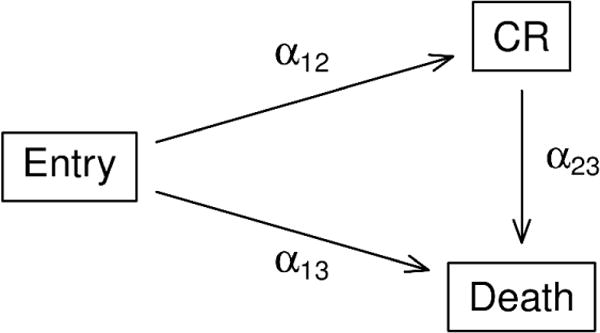
a. Multi-state model structure of simulation study

CR: complete remission

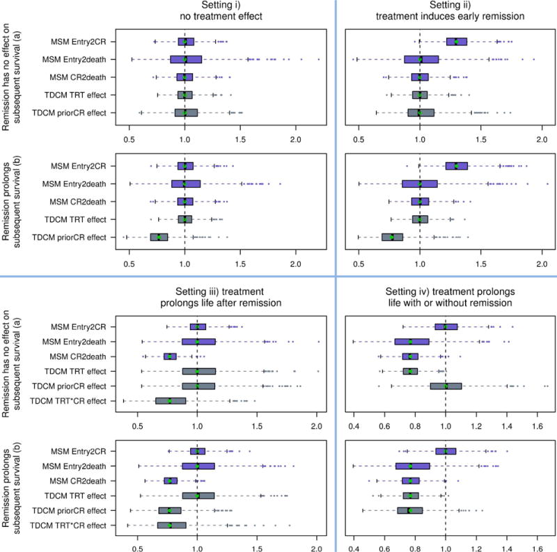
b. Box-plot of estimated hazard ratios for eight simulated scenarios

MSM: multi-state model, Entry2CR: study entry to complete remission, Entry2death: study entry to death, CR2death: complete remission to death, TDCM: time-dependent Cox model, prior CR: effect of complete remission on mortality, TRT: treatment, and TRT*CR: interaction between the treatment effect and the effect of complete remission on mortality

Simulation results

Figure 4b shows the box-plots of the estimated hazard ratios of the treatment effects of three transitions: entry to complete remission, entry to death, and complete remission to death using the Cox-type regression under the multi-state model (labeled as MSM Entry2CR, MSM Entry2death, MSM CR2death, respectively). The box-plots of the estimated hazard ratios of the effect of the time-dependent covariate complete remission and of the treatment effect on survival using the time-dependent Cox model (labeled as TDCM priorCR effect and TDCM TRT effect, respectively) are shown alongside the multi-state model results. In these plots, the vertical dashed lines denote the reference hazard ratio of 1 which means equal risk. The green dots show the hazard ratio under the true model. Tables 2 shows the probability of rejecting the null hypothesis corresponding to the two analyses methods for the four scenarios in set a) where complete remission has no effect on subsequent survival. Similar conclusions can be drawn from set b) hence results are not shown.

Setting i) no treatment effect (upper left quadrant of Figure 4b)

The hazard ratios for all transitions in the multi-state model in this setting centered around 1 as expected in both panels. In scenario a), (upper panel), results from the time-dependent Cox model indicated neither effect of complete remission nor of treatment on survival as expected. In this scenario (first row of Table 3), these probabilities correspond to the Type I errors and they were all close to 5%. In scenario b), (lower panel), the estimated hazard ratios of the effect of complete remission on subsequent survival centered around 0.77 which was the true hazard ratio set in the simulation.

Table 3.

Probability of rejecting the null hypothesis under scenarios where remission has no effect on subsequent survival

	Multi-state Cox-type regression			Time-dependent Cox regression
	Entry to complete remission	Entry to death	Complete remission to death	Treatment	Prior complete remission	Interaction between treatment and prior complete remissiona
setting i) no treatment effect	0.046	0.057	0.046	0.054	0.056	–
setting ii) treatment induces early remission	0.758	0.05	0.046	0.058	0.051	–
setting iii) treatment prolongs life after remission	0.049	0.05	0.735	0.054	0.056	0.222
setting iv) treatment prolongs life with or without remission	0.058	0.219	0.763	0.835	0.05	–

^aOnly included for setting iii

Setting ii) treatment induces early complete remission (upper right quadrant of Figure 4b)

Both panels show a higher transition rate from entry to complete remission in the treatment group with the estimated hazard ratios centered around 1.3 (the true value set in the simulation) and no increased risk of death from complete remission or from entry, all as expected. Table 3 (setting ii), Entry to complete remission) shows a 76% likelihood (power) to detect an increase in complete remission rate. The Type I errors for other comparisons were all close to 0.05 as expected. Since complete remission had no effect on survival in scenario a), (upper panel), the estimated hazard ratios of both treatment and complete remission centered around 1. In scenario b), (lower panel), where complete remission was associated with lower risk of mortality, the estimates hazard ratios of complete remission in the time-dependent Cox model centered around 0.77 which was the true value. In this scenario, the time-dependent Cox model did well in estimating the effect of complete remission on survival.

Setting iii) treatment prolongs life after complete remission (lower left quadrant of Figure 4b)

The multi-state models in both panels, again, performed well in detecting the treatment effect on all transitions with the hazard ratios centered near the true values. The estimated hazard ratios for the complete remission-to-death transition centered around 0.77 while the hazard ratios for other transitions centered around 1. An interaction term between treatment and complete remission was added to the time-dependent Cox model in setting iii) to ensure the model was correctly specified. As a result, the time-dependent Cox model with the interaction term performed well, with the estimated hazard ratios centered near their true values for both scenarios a) and b). It is important to note, however, that without the interaction term (results not shown), the time-dependent Cox model overestimates the effect of complete remission and underestimates the effect of treatment on survival in this setting. The bias from the time dependent Cox model without an interaction term is a consequence of the model picking up the effect of treatment on survival post-complete remission as an effect of complete remission itself on survival. The addition of the interaction term allows the time-dependent Cox model to account for the differential treatment effects before and after complete remission. Although adding the interaction term to the time-dependent Cox model led to unbiased estimation of the treatment effect post complete remission, as shown in the lower left quadrant of Figure 4b, the variance of the estimated treatment effect for this model can be large compared to the variance of the estimated treatment effect from the multi-state model analysis. As a consequence, the power to detect the treatment effect after complete remission was lower (22.2%) in the time-dependent Cox model compared to the power to detect the treatment effect (73.5%) in the complete remission-to-death transition in the multi-state model (third row of Table 3). In settings where there is no differential treatment effects by occurrence of complete remission (settings i, ii, and iv), the variance of the estimated treatment effect in the time-dependent Cox model without the interaction term was smaller than the variance of the estimated treatment effects from the multi-state models. As suggested by a reviewer, in practice, one could first test for presence of interaction and include the interaction term if needed.

Setting iv) treatment prolongs life with or without complete remission (lower right quadrant of Figure 4b)

Again, the multi-state model performed well with the estimated hazard ratios centered around the true value for all transitions in both panels. However, the power comparing the transition rates from entry to death was relatively low (21.9%, setting iv) of Table 3). This is due to the low number of patients experienced this transition because the scenario was set up where 80% of patients would achieve complete remission and only 20% would go from entry to death. The time-dependent Cox model performed well in this setting with the estimated hazard ratios of both complete remission and treatment centered near their true value. Since treatment prolongs life regardless of complete remission status in this setting, improvement in survival occurred in the treatment arm both with and without complete remission. Therefore, the time-dependent Cox model without the interaction term performed well estimating the effect of complete remission on survival.

Results from these simulated scenarios illustrate the differences between multi-state models and time-dependent Cox models. Multi-state models evaluate the effect of treatment on all possible transitions where the end states of the transitions are outcomes in the models. Specifically, in the simulated example, complete remission and death were two outcomes in the multi-state models, whereas death was the only outcome in the time-dependent Cox models. In this context, multi-state models can help answer the question of whether the treatment can lead to a faster complete remission; whereas the time-dependent Cox models can answer the question of whether having achieved complete remission can improve survival beyond the effect of treatment. It is worth noting that the effect of complete remission on survival cannot be estimated by the multi-state model in this setting because complete remission is one of the states rather than a covariate in the multi-state models.

Discussion

Software for multi-state model analysis

Multiple software packages in R work well in specific cases but have limitation in others. The survival package²¹ is capable of seamlessly performing restricted mean time in state analysis, though the implementation of multi-state Cox models can be more difficult for complex multi-state structures. The mstate package^{22, 23} (which is a set of helper functions for using the survival package to do multistate analysis) is a useful add-on for the survival package²¹ that attempts to simplify the Cox modeling process. The mstate package^{22, 23} also facilitates the plotting of predicted probabilities from these multi-state models. While we did not investigate its use, the msm package²⁴ is also useful for handling interval censoring and hidden Markov models.

It is often worthwhile in multi-state analysis to simulate new data under various assumptions to gain a perspective on the power and the family-wise error rate in multi-state models. There are several software packages that can aid in this respect. The simMSM R package²⁰ allows great flexibility in parameterizing multi-state analysis, we found that the documentation is somewhat sparse. The Multistate Simulation Designer¹⁹ is an open-source web application coded in R’s shiny package²⁵ which was created to simplify this simulation process (the application is available at https://ph-shiny.iowa.uiowa.edu/rpterson/MSDshiny/). While less general than the simMSM package,²⁰ the flow of the application is simple and straightforward.

For our analysis, we used the mstate^{22, 23} and survival²¹ packages. For our simulations, we used the Multistate Simulation Designer, as well as the simMSM package.²⁰ The mstate^{22, 23} and survival²¹ packages both have very useful vignettes for how to perform multi-state modeling wherein code is presented and the results are interpreted. These vignettes are available on the CRAN website or directly in the source files for these packages.

Conclusion

This article illustrates multi-state model analyses of data from a recently published clinical trial.⁵ The primary analysis of this dataset using standard Cox regression model showed that midostaurin was associated with an improvement in overall survival and disease-free survival. However, there are multiple intermediate events that can happen to patients between trial enrollment and death. The total time course from the initial state of trial enrollment to final endpoint of death can thus be broken up into mutually exclusive transitions. Multi-state models is an analysis tool that allows examination of the effect of treatment on each of these transitions. These analyses suggested that the overall survival advantage of midostaurin over placebo was due to its association with a higher first complete remission rate and a lower risk of relapse and death for patients who achieved first complete remission.

Although multi-state models were introduced 40 years ago and are a well-known topic in survival analysis, multi-state analyses are not commonly used in practice. Their slow adaptation can be attributed to the lack of proprietary software that can fit multi-state models, or to medical research community’s attachment to the standard Kaplan-Meier estimator or the Cox models, or to the complexity of the multi-state model framework. Multiple software packages are available to conduct this type of analyses, especially the R survival package²¹ which is an easy to use, well-maintained open-source software with clearly documented vignettes for users.

Multi-state models can be used as a complementary tool to standard survival analyses routines to paint a more comprehensive picture of the treatment effect and to gain a better understanding of the disease process. Although it is true that a multi-state model can get complicated with a large number of states and, with a large number of transitions, the numbers of patients at risk for the latter transitions can get small for meaningful inferences. However, as with any statistical models, it is important to strike a balance between complexity and utility.

References

- 1.Kaplan EL, Meier P. Nonparametric estimation from incomplete observations. J Am Stat Assoc. 1958;53:457–481. [Google Scholar]
- 2.Kalbfleisch JD, Prentice RL. The statistical analysis of failure time data. New York: Wiley; 1980. p. xi. 321 p. [Google Scholar]
- 3.Cox DR. Regression models and life-tables. J R Stat Soc Series B Stat Methodol. 1972;34:187–220. [Google Scholar]
- 4.Fine JP, Gray RJ. A proportional hazards model for the subdistribution of a competing risk. J Am Stat Assoc. 1999;94:496–509. [Google Scholar]
- 5.Stone RM, Mandrekar SJ, Sanford BL, et al. Midostaurin plus chemotherapy for acute myeloid leukemia with a FLT3 mutation. N Engl J Med. 2017;377:454–464. doi: 10.1056/NEJMoa1614359. [DOI] [PMC free article] [PubMed] [Google Scholar]
- 6.Aalen OO, Johansen S. An empirical transition matrix for non-homogeneous Markov chains based on censored observations. Scand J Stat. 1978;5:141–150. [Google Scholar]
- 7.Andersen PK, Gill RD, Keiding N. Statistical models based on counting processes. New York: Springer; 1993. [Google Scholar]
- 8.Klein JP, Keiding N, Copelan EA. Plotting summary predictions in multistate survival models: probabilities of relapse and death in remission for bone marrow transplantation patients. Stat Med. 1993;12:2315–2332. doi: 10.1002/sim.4780122408. [DOI] [PubMed] [Google Scholar]
- 9.Hougaard P. Multi-state models: a review. Lifetime Data Anal. 1999;5:239–264. doi: 10.1023/a:1009672031531. [DOI] [PubMed] [Google Scholar]
- 10.Commenges D. Multi-state models in epidemiology. Lifetime Data Anal. 1999;5:315–327. doi: 10.1023/a:1009636125294. [DOI] [PubMed] [Google Scholar]
- 11.Andersen PK, Keiding N. Multi-state models for event history analysis. Stat Methods Med Res. 2002;11:91–115. doi: 10.1191/0962280202SM276ra. [DOI] [PubMed] [Google Scholar]
- 12.Putter H, Fiocco M, Geskus RB. Tutorial in biostatistics: Competing risks and multi-state models. Stat Med. 2007;26:2389–2430. doi: 10.1002/sim.2712. [DOI] [PubMed] [Google Scholar]
- 13.Andersen PK, Keiding N. Interpretability and importance of functionals in competing risks and multistate models. Stat Med. 2012;31:1074–1088. doi: 10.1002/sim.4385. [DOI] [PubMed] [Google Scholar]
- 14.van den Hout A. Multi-state survival models for interval-censored data. Boca Raton: Chapman and Hall/CRC; 2016. [Google Scholar]
- 15.Xia F, George SL, Wang X. A multi-state model for designing clinical trials for testing overall survival allowing for crossover after progression. Stat Biopharm Res. 2016;8:12–21. doi: 10.1080/19466315.2015.1093539. [DOI] [PMC free article] [PubMed] [Google Scholar]
- 16.Stephens-Shields AJ, Spieker AJ, Anderson A, et al. Blood pressure and the risk of chronic kidney disease progression using multistate marginal structural models in the CRIC Study. Stat Med. 2017;36:4167–4181. doi: 10.1002/sim.7425. [DOI] [PMC free article] [PubMed] [Google Scholar]
- 17.Jepsen P, Vilstrup H, Andersen PK. The clinical course of cirrhosis: The importance of multistate models and competing risks analysis. Hepatology. 2015;62:292–302. doi: 10.1002/hep.27598. [DOI] [PubMed] [Google Scholar]
- 18.Willeumier JJ, Rueten-Budde AJ, Jeys LM, et al. Individualised risk assessment for local recurrence and distant metastases in a retrospective transatlantic cohort of 687 patients with high-grade soft tissue sarcomas of the extremities: a multistate model. BMJ Open. 2017;7:e012930. doi: 10.1136/bmjopen-2016-012930. [DOI] [PMC free article] [PubMed] [Google Scholar]
- 19.Peterson RA. The multistate simulation designer, GitHub repository. https://github.com/petersonR/MSDshiny (2017 accessed 21 June 2018)
- 20.Reulen H. SimMSM: Simulation of event histories for multi-state models. R package version 1.1.41. https://CRAN.R-project.org/package=simMSM (2015, accessed 21 June 2018)
- 21.Therneau TM. A package for survival analysis in S. R package version 2.38. https://CRAN.R-project.org/package=survival (2015, accessed 21 June 2018)
- 22.de Wreede LC, Fiocco M, Putter H. The mstate package for estimation and prediction in non- and semi-parametric multi-state and competing risks models. Comput Methods Programs Biomed. 2010;99:261–274. doi: 10.1016/j.cmpb.2010.01.001. [DOI] [PubMed] [Google Scholar]
- 23.de Wreede LC, Fiocco M, Putter H. mstate: An R package for the analysis of competing risks and multi-state models. J Stat Softw. 2011;38:1–30. [Google Scholar]
- 24.Jackson C. Multi-state models for panel data: The msm package for R. J Stat Softw. 2011;38:1–29. [Google Scholar]
- 25.Chang W, Cheng J, Allaire J, et al. Shiny: Web application framework for R. R package version 1.0.5. https://CRAN.R-project.org/package=shiny (2016, accessed 21 June 2018)
Associated Data
This section collects any data citations, data availability statements, or supplementary materials included in this article.