httk: R Package for High-Throughput Toxicokinetics

Abstract

Thousands of chemicals have been profiled by high-throughput screening programs such as ToxCast and Tox21; these chemicals are tested in part because most of them have limited or no data on hazard, exposure, or toxicokinetics. Toxicokinetic models aid in predicting tissue concentrations resulting from chemical exposure, and a “reverse dosimetry” approach can be used to predict exposure doses sufficient to cause tissue concentrations that have been identified as bioactive by high-throughput screening. We have created four toxicokinetic models within the R software package httk. These models are designed to be parameterized using high-throughput in vitro data (plasma protein binding and hepatic clearance), as well as structure-derived physicochemical properties and species-specific physiological data. The package contains tools for Monte Carlo sampling and reverse dosimetry along with functions for the analysis of concentration vs. time simulations. The package can currently use human in vitro data to make predictions for 553 chemicals in humans, rats, mice, dogs, and rabbits, including 94 pharmaceuticals and 415 ToxCast chemicals. For 67 of these chemicals, the package includes rat-specific in vitro data. This package is structured to be augmented with additional chemical data as they become available. Package httk enables the inclusion of toxicokinetics in the statistical analysis of chemicals undergoing high-throughput screening.

1. Introduction

Humans are exposed to thousands of chemicals from the environment and consumer products, most of which have not been tested for toxicity (Park et al. 2012; Wambaugh et al. 2013b; Egeghy et al. 2011; Judson et al. 2008). In order to screen for potential bioactivity, in vitro data have been generated in the Tox21 (Bucher 2008) and ToxCast (Judson et al. 2010) programs using high-throughput screening systems. Over 8500 chemicals have been tested in at least 50 assays (Tox21), and a subset of around 1800 have had nearly 1200 assay endpoints measured (ToxCast). Recently, high-throughput exposure modeling has provided estimates of daily human exposure for thousands of environmental contaminants (Wambaugh et al. 2014). However, linking these hazard and exposure predictions to estimate risk requires development and use of high-throughput toxicokinetics. The terms “pharmacokinetic”, “toxicokinetic”, and “biokinetic” models have been used somewhat interchangeably in the scientific literature. However, since this package is intended to provide dose context to high-throughput toxicity screening projects, we have selected the term “toxicokinetic” even though we include several compounds with known therapeutic benefits and many others that may not cause adversity for the highest plausible dose.

Toxicokinetics is a field of study for determining the absorption, distribution, metabolism, and excretion of substances in the body (O’Flaherty 1981). The necessary data for toxicokinetics are commonly collected in rats and other animals, but the collection of these data for thousands of chemicals is costly in time, money, and animals (Rovida and Hartung 2009). Creating computational predictive models parameterized with more easily obtained in vitro data may help address these problems. Inputting estimated exposures into toxicokinetic models yields information about the steady state and time course concentrations in various parts of the body. These concentrations can then be compared to concentrations that cause biological activity in in vitro assays. The models can also be used in a reverse manner, known as reverse toxicokinetics, by predicting the dose needed to produce a specific concentration of interest, such as the in vitro AC₅₀ or other levels of biological activity as done in Wetmore et al. (2012) and Wetmore (2015). Thus chemicals can be ranked based on the ratio of the predicted exposure dose to the back-calculated bioactive dose (Thomas et al. 2013), which, due to the linearity of these models, is equal to the ratio of the predicted steady state concentration to the in vitro bioactive concentration.

Many basic toxicokinetic models (Wetmore et al. 2012; Wetmore 2015; Pelekis et al. 1997) only predict steady state plasma concentrations (C_ss), assuming a dose rate that is both continuous and constant (e.g., infusion dose). With a more dynamic model, such as a physiologically based toxicokinetic (pbtk) model, we can simulate discrete doses to reach steady state, which we observe to oscillate around the infusion dose prediction. Our pbtk models include multiple compartments with partition coefficients. These models are expressed as a set of mass balance differential equations describing the rate of change of the amount of a substance in each compartment. Chemical-specific physicochemical data and species-specific in vitro and physiological data are used in calculating the partition coefficients, clearance, tissue volumes, and blood flows. These in vitro data consist of the intrinsic hepatic clearance, Cl_int, and the plasma protein binding, f_ub. httk provides tools for Monte Carlo sampling and reverse dosimetry (Tan et al. 2006) along with functions that solve for concentration vs. time curves, steady state concentrations, the number of days to steady state, and other toxicokinetic summary statistics for chemicals as shown in Tables 4 and Table 5 with the corresponding abbreviations in Table 1. With this R package we provide data, models, and examples to allow the inclusion of toxicokinetics in statistical analysis of chemical exposure and toxicity for 553 chemicals. The package is structured to be modular and expandable to allow new modeling approaches and chemical data to be added as they become available.

Table 4:

List of functions in the package – Part I. Models are described in Table 2. Parameters are defined in Table 1. Jarnac and SBML are external languages for systems biology models.

Function	Description
add_chemtable	Adds a table of chemical data to the data tables contained in the package.
available_rblood2plasma	.Retrieves best available Rbiood2piasma, using get_rblood2plasma and calc_rblood2plasma.
calc_analytic_css	Calculates Css and blood concentrations for the four models used in the package from infusion dosing at a constant rate.
calc_css	Calculates the maximum and average steady state concentrations along with the day steady state is reached from the numerical solution.
calc_elimination_rate	Calculates kelim for a one compartment model due to the liver and kidneys, dividing the total clearance by Vdist.
calc_hepatic_clearance	Calculates the hepatic clearance for a well-stirred model or other type if specified (Ito and Houston 2004).
calc_mc_css	Calculates Css using Monte Carlo simulation, defaulting to HTTK-Pop simulator (Ring et al. 2017).
calc_mc_oral_equiv	Converts Css to an oral equivalent dose using a concentration obtained from calc_mc_css.
calc_rblood2plasma	Calculates the ratio of chemical concentration in blood to plasma.
calc_stats	Calculates the area under the curve, mean, and peak values for the blood or plasma concentration of either a specified chemical or all chemicals for a given simulation.
calc_total_clearance	Calculates the total clearance rate for a one compartment model where clearance is equal to the sum of the well-stirred metabolism by the liver and glomerular filtration in the kidneys.
calc_vdist	Calculates the volume of distribution for a one compartment model (Schmitt 2008b).
export_pbtk_jarnac	Exports the model pbtk to Jarnac (Sauro and Fell 2000).
export_pbtk_sbml	Exports the model pbtk to SBML (Hucka et al. 2003).
get_cheminfo	Provides a list of CAS numbers along with compound names, logP, pKa, molecular weight, Clint and its p value, and fub if specified for chemicals with sufficient data for a given model.
get_httk_params	Converts table generated by httkpop_generate to the corresponding table of httk model parameters.
get_rblood2plasma	Retrieves in vivo Rblood2plasma.
get_wetmore_cheminfo	Provides the names and CAS numbers of chemicals with information from Wetmore et al. (2012), Wetmore et al. (2013), and Wetmore (2015).
get_wetmore_css	Retrieves Css as a result of oral infusion dosing from Wetmore et al. (2012), Wetmore et al. (2013), and Wetmore (2015).
get_wetmore_oral_equiv	Converts Css to an oral equivalent dose using the values from Wetmore et al. (2012), Wetmore et al. (2013), and Wetmore (2015).
httkpop_generate lump_tissues	Generates a virtual population. Lumps tissue flows, volumes, and input partition coefficients based on specified grouping.

Table 5:

List of functions in the package – Part II. Models are described in Table 2. Parameters are defined in Table 1. Jarnac and SBML are external languages for systems biology models.

Function	Description
monte_carlo	Runs a Monte Carlo simulation of a given model.
parameterize_1comp	Parameterizes the model 1compartment.
parameterize_3comp	Parameterizes the model 3compartment.
parameterize_pbtk	Parameterizes the model pbtk.
parameterize_schmitt	Parameterizes predict_partitioning_schmitt.
parameterize_steadystate	Parameterizes the model 3compartmentss, used in Wetmore et al. (2012) and Wetmore (2015).
predict_partitioning_schmitt	Predicts partition coefficients using Schmitt’s method (Schmitt 2008b).
solve_1comp	Solves the model 1compartment.
solve_3comp	Solves the model 3compartment.
solve_pbtk	Solves the model pbtk.

Table 1:

List of abbreviations.

Variable	Name
1compartment	One compartment model (O’Flaherty 1981), shown in Figure 1.
3compartment	Three compartment model (Jamei et al. 2009), shown in Figure 1.
3compartmentss	Three compartment steady state model (Wetmore et al. 2012; Wetmore 2015).
BW	Body weight.
Css	Average plasma concentration of a chemical at steady state.
Clint	In vitro intrinsic hepatic clearance.
Clmetabolism	Whole liver hepatic clearance, scaled from Clint.
Clwell–stirred	Hepatic clearance modeled with well-stirred approximation using Clmetabolism.
fub	Fraction unbound, in vitro ratio of unbound to total concentration in plasma.
httk	High-throughput toxicokinetics.
kelim	Elimination rate.
kgutabs	Gut absorption rate, default of 1 h−1.
logP	Logarithm (base 10) of octanol to water partition coefficient.
pbtk	Physiologically based toxicokinetic model, shown in Figure 1.
Qcardiac	Cardiac output, blood flow through the heart and lungs.
Qgfr	Glomerular filtration rate.
Qrest	The difference between Qcardiac and the flow to the liver, kidney, and gut.
Qtissue	Blood flow to a tissue.
QSAR	Quantitative structure-activity relationship.
Rblood2plasma	Ratio of the blood concentration of a chemical to the plasma concentration.
SBML	Systems biology markup language.
SMILES	Simplified molecular-input line-entry system.
Vdist	Volume of distribution, the weighted sum of all partition coefficients.

2. Methods

Version 1.7 of httk (Wambaugh and Pearce 2016) is used in this manuscript. The package is available from the Comprehensive R Archive Network (CRAN) at https://CRAN.R-project.org/package=httk.

2.1. Models included

The four models in httk include: “pbtk”, “3compartment”, “3compartmentss”, and “1compartment”; the predictions and parameters of these models are compared in Table 2. All models currently use only oral and intravenous (i.v.) dosing. The models pbtk and 3compartment, shown in Figure 1, use tissue to unbound plasma partition coefficients calculated with a modified version of Schmitt’s model (Schmitt 2008b; Pearce et al. 2017) (using octanol-water partitioning, membrane affinity, acid/base dissociation constants, tissue compositions, and adjusted f_ub) to simulate chemical concentrations over time for multiple tissue compartments. The model pbtk contains separate tissue compartments for the gut, liver, lungs, arteries, veins, and kidneys while the model 3compartment only contains compartments for the liver and gut and is essentially a condensed form of the model pbtk. The tissues contained in tissue.data that are unused in each of these models are aggregated into a single compartment termed “rest”, whose partition coefficient is calculated by averaging the remaining partition coefficients, weighted by their species-specific tissue volumes. Absorption from the gut lumen into gut tissue is modeled as a first order process with an arbitrary “fast” absorption rate of 1 h⁻¹. The fraction of the dose absorbed into the system through the gut wall is set to 1 when measured data are unavailable. The gut blood flows directly into the liver, where the hepatic clearance, Cl_metabolism, is calculated with a unit conversion of Cl_int using the density of hepatocytes in the liver (1.1 × 10⁸ hepatocytes per gram of liver from Ito and Houston 2004 and a liver density of 1.05 g/mL from Snyder et al. 1975). Both models also feature renal elimination by passive glomerular filtration through the kidneys. We assume perfusion-limited tissue (i.e., tissue, red blood cells, and plasma come to equilibrium rapidly with respect to the flow of blood), and a constant R_blood2plasma is used throughout the body, predicted using hematocrit and the predicted partitioning between red blood cells and plasma when in vivo values are unavailable.

Table 2:

Model parameter and prediction comparison.

Model	Hepatic clearance	Partition coefficients	Fraction unbound	Hematocrit	Molecular weight	Ratio of blood to plasma	Elimination rate*	Volume of distribution*	Dynamic prediction	Steady state prediction
pbtk	Yes	Yes	Yes	Yes	Yes	Yes	No	No	Yes	Yes
1compartment	No	No	No	No	Yes	No	Yes	Yes	Yes	Yes
3compartment	Yes	Yes	Yes	Yes	Yes	Yes	No	No	Yes	Yes
3compartmentss	Yes	No	Yes	No	Yes	No	No	No	No	Yes

^*Partition coefficients are needed in calculating V_dist. Clearances and f_ub are needed in calculating k_elim.

Figure 1:

Models (A) 1compartment, (B) 3compartment, and (C) pbtk. In order to preserve mass-balance, Q_rest is defined as the difference between Q_cardiac and the flow to the liver, kidney, and gut. Variable names are defined in Table 1.

The models 3compartmentss and 1compartment both contain only plasma without separate compartments for blood and tissue (and thus no individual partition coefficients). The model 3compartmentss, “ss” standing for steady state, is a single equation for the C_ss of the rest-of-body compartment in the model 3compartment resulting from i.v. dosing. This is the same equation used for determining C_ss in previous work (Rotroff et al. 2010; Wetmore et al. 2012; Wetmore 2015; Wilkinson and Shand 1975) but with a modification adjusting for the misuse of hepatic blood flow in determining plasma clearance (Yang et al. 2007). The model 1compartment features an absorption compartment and a total clearance equal to the sum of the metabolism of the parent compound in the liver, modeled with the adjusted “well-stirred” approximation (Wilkinson and Shand 1975; Houston and Carlile 1997), and the renal clearance by passive glomerular filtration. The elimination rate, k_e, is equal to the total clearance divided by the volume of distribution, V_dist. V_dist is used as the volume of the compartment and is calculated by summing the plasma volume and the products of each tissue to unbound plasma partition coefficient, its corresponding volume, and f_ub (Schmitt 2008b). C_ss resulting from infusion dosing for the model 1compartment is equivalent to 3compartmentss.

Among the four models in the package, the simplest model, 3compartmentss, is applicable to the largest number of chemicals, specifically those which are missing information needed to parameterize the other models. It is the only model that does not use partition coefficients and thus does not require logP, and when f_ub is below the limit of detection, the model can be used with Monte Carlo to simulate C_ss distributions. Thus, f_ub below the limit of detection (set to zero in chem.physical_and_invitro.data and 0.005 in default parameter lists) and Cl_int are the minimum data requirements for running a model. The model 1compartment is included to compare our predictions with in vivo experiments which are often characterized by one compartment model parameters (V_dist and k_elim). We note that fully understanding the kinetics of a given chemical might require additional data on features currently not accessible with high-throughput in vitro approaches, such as bioavailability, transporters, protein-binding kinetics, and extra-hepatic or strongly saturable metabolism (Rotroff et al. 2010).

2.2. Model equations

The differential equations below describe changes in the concentrations or amounts of a substance within the model compartments. Although the models are written as changes in tissue concentrations, except for the gut lumen, the equations actually express changes in the amount of substance in the blood of each tissue divided by the tissue volume with the blood and tissue concentrations related through the out-flowing concentration in blood. A blood flow, Q (L/day), multiplied by a concentration, C (mol/L), is equal to the amount of the substance entering or leaving a compartment through the blood, QC (mol/day). We define partition coefficients as the ratio of the concentration in a tissue to the unbound concentration in plasma of that tissue; K_tissue2pu = C_tissue/(f_ub C_plasma). Thus dividing C_tissue by K_tissue2pu and f_ub and then multiplying by R_blood2plasma yields the blood concentration of the compartment at equilibrium, C_tissue R_blood2plasma/(f_ub K_tissue2pu). Assuming perfusion-limited tissue, we substitute this term for the out-flowing blood concentrations (Campbell Jr et al. 2012) and assume negligible blood volume fractions in all tissues to justify dividing by the tissue volume without a blood volume fraction and partition coefficient dependency. The flow to the rest-of-body, Q_rest, is calculated by subtracting the sum of all the other tissue flows (i.e., gut, liver, and kidney) from the total cardiac output. The glomerular filtration rate, Q_gfr, and the hepatic clearance, Cl_metabolism, (both in L/day) are both multiplied by the unbound plasma concentrations, C_tissue/K_tissue2pu, in the kidney and liver to express the amount of the substance leaving the system. Note that although the units of the clearances, flows, and absorption rate are in days, being consistent with the model outputs, they are initially entered in units of hours. The model 3compartmentss assumes a constant dose rate, k_dose (mg/kg BW/day), and the other models use discrete changes in the amount in the gut lumen or venous concentration, depending on which type of dose is specified. The function that is part of the gut lumen equation, g(t) describes the oral dosing schedule. MCSim (Bois and Maszle 1997) was used for converting the model equations into C code, which is used with deSolve (Soetaert et al. 2016) in solving each system of equations.

pbtk equations

$$\begin{array}{cc}\hfill & \frac{d}{dt}{A}_{\mathit{gutlumen}}=-k_{\mathit{gutabs}}{A}_{\mathit{gutlumen}}+g(t)\hfill \\ \hfill & \frac{d}{dt}{C}_{\mathit{gut}}=\left(k_{\mathit{gutabs}}{A}_{\mathit{gutlumen}}+Q_{\mathit{gut}}\left(C_{\mathit{art}}-\frac{R_{\mathrm{blood}2\mathrm{plasma}}}{K_{\mathrm{gut}2\mathrm{pu}}{f}_{ub}}{C}_{\mathit{gut}}\right)\right)/V_{\mathit{gut}}\hfill \\ \hfill & \frac{d}{dt}{C}_{\mathit{liver}}=\left(Q_{\mathit{liver}}{C}_{\mathit{art}}+\frac{Q_{\mathit{gut}}{R}_{\mathrm{blood}2\mathrm{plasma}}}{K_{\mathrm{gut}2\mathrm{pu}}{f}_{\mathit{ub}}}{C}_{\mathit{gut}}-\frac{(Q_{\mathit{liver}}+Q_{\mathit{gut}})R_{\mathrm{blood}2\mathrm{plasma}}}{K_{\mathrm{liver}2\mathrm{pu}}{f}_{\mathit{ub}}}{C}_{\mathit{liver}}-\frac{C{l}_{\mathit{metabolism}}}{K_{\mathrm{liver}2\mathrm{pu}}}{C}_{\mathit{liver}}\right)/V_{\mathit{liver}}\hfill \\ \hfill & \frac{d}{dt}{C}_{\mathit{ven}}=\left(\left(\frac{Q_{\mathit{liver}}+Q_{\mathit{gut}}}{K_{\mathrm{liver}2\mathrm{pu}}}{C}_{\mathit{liver}}+\frac{Q_{\mathit{kidney}}}{K_{\mathrm{kidney}2\mathrm{pu}}}{C}_{\mathit{kidney}}+\frac{Q_{\mathit{rest}}}{K_{\mathrm{rest}2\mathrm{pu}}}{C}_{\mathit{rest}}\right)\frac{R_{\mathrm{blood}2\mathrm{plasma}}}{f_{\mathit{ub}}}-Q_{\mathit{cardiac}}{C}_{\mathit{ven}}\right)/V_{\mathit{ven}}\hfill \\ \hfill & \frac{d}{dt}{C}_{\mathit{lung}}=Q_{\mathit{cardiac}}\left(C_{\mathit{ven}}-\frac{R_{\mathrm{blood}2\mathrm{plasma}}}{K_{\mathrm{lung}2\mathrm{pu}}{f}_{\mathit{ub}}}{C}_{\mathit{lung}}\right)/V_{\mathit{lung}}\hfill \\ \hfill & \frac{d}{dt}{C}_{\mathit{art}}=Q_{\mathit{cardiac}}\left(\frac{R_{\mathrm{blood}2\mathrm{plasma}}}{K_{\mathrm{lung}2\mathrm{pu}}{f}_{\mathit{ub}}}{C}_{\mathit{lung}}-C_{\mathit{art}}\right)/V_{\mathit{art}}\hfill \\ \hfill & \frac{d}{dt}{C}_{\mathit{rest}}=Q_{\mathit{rest}}\left(C_{\mathit{art}}-\frac{R_{\mathrm{blood}2\mathrm{plasma}}}{K_{\mathrm{rest}2\mathrm{pu}}{f}_{\mathit{ub}}}{C}_{\mathit{rest}}\right)/V_{\mathit{rest}}\hfill \\ \hfill & \frac{d}{dt}{C}_{\mathit{kidney}}=\left(Q_{\mathit{kidney}}{C}_{\mathit{art}}-\frac{Q_{\mathit{Kidney}}{R}_{\mathrm{blood}2\mathrm{plasma}}}{K_{\mathrm{kidney}2\mathrm{pu}}{f}_{\mathit{ub}}}{C}_{\mathit{kidney}}-\frac{Q_{\mathit{gfr}}}{K_{\mathrm{kidney}2\mathrm{pu}}}{C}_{\mathit{kidney}}\right)/V_{\mathit{kidney}}\hfill \end{array}$$

3compartment equations

$$\begin{array}{cc}\hfill & \frac{d}{dt}{A}_{\mathit{gutlumen}}=-k_{\mathit{gutabs}}{A}_{\mathit{gutlumen}}+g(t)\hfill \\ \hfill & \frac{d}{dt}{C}_{\mathit{gut}}=\left(k_{\mathit{gutabs}}{A}_{\mathit{gutlumen}}+\frac{Q_{\mathit{gut}}{R}_{\mathrm{blood}2\mathrm{plasma}}}{K_{\mathrm{rest}2\mathrm{pu}}{f}_{\mathit{ub}}}{C}_{\mathit{rest}}-\frac{Q_{\mathit{gut}}{R}_{\mathrm{blood}2\mathrm{plasma}}}{K_{\mathrm{gut}2\mathrm{pu}}}{f}_{\mathit{ub}}{C}_{\mathit{gut}}\right)/V_{\mathit{gut}}\hfill \\ \hfill & \frac{d}{dt}{C}_{\mathit{liver}}=\left(\frac{Q_{\mathit{gut}}{R}_{\mathrm{blood}2\mathrm{plasma}}}{K_{\mathrm{gut}2\mathrm{pu}}{f}_{\mathit{ub}}}{C}_{\mathit{gut}}+\frac{Q_{\mathit{liver}}{R}_{\mathrm{blood}2\mathrm{plasma}}}{K_{\mathrm{rest}2\mathrm{pu}}{f}_{\mathit{ub}}}{C}_{\mathit{rest}}-\left(\frac{(Q_{\mathit{liver}}+Q_{\mathit{gut}})R_{\mathrm{blood}2\mathrm{plasma}}}{f_{\mathit{ub}}{K}_{\mathrm{liver}2\mathrm{pu}}}+\frac{C{l}_{\mathit{metabolism}}}{K_{\mathrm{liver}2\mathrm{pu}}}\right)C_{\mathit{liver}}\right)/V_{\mathit{liver}}\hfill \\ \hfill & \frac{d}{dt}{C}_{\mathit{rest}}=\left(\frac{(Q_{\mathit{gut}}+Q_{\mathit{liver}})R_{\mathrm{blood}2\mathrm{plasma}}}{f_{\mathit{ub}}{K}_{\mathrm{liver}2\mathrm{pu}}}{C}_{\mathit{liver}}-\left(\frac{R_{\mathrm{blood}2\mathrm{plasma}}}{f_{\mathit{ub}}}(Q_{\mathit{gut}}+Q_{\mathit{liver}})+Q_{\mathit{gfr}}\right)\frac{C_{\mathit{rest}}}{K_{\mathrm{rest}2\mathrm{pu}}}\right)/V_{\mathit{rest}}\hfill \end{array}$$

1compartment equations

$$\begin{array}{cc}\hfill & \frac{d}{dt}{A}_{\mathit{gutlumen}}=-k_{\mathit{gutabs}}{A}_{\mathit{gutlumen}}+g(t)\hfill \\ \hfill & \frac{d}{dt}{C}_{\mathit{rest}}=\frac{k_{\mathit{gutabs}}}{V_{\mathit{dist}}}{A}_{\mathit{gutlumen}}-k_{\mathit{elim}}{C}_{\mathit{rest}}\hfill \end{array}$$

3compartmentss equation

$$C_{\mathit{ss}}=k_{\mathit{dose}}/\left(f_{\mathit{ub}}{Q}_{\mathit{gfr}}+\frac{(Q_{\mathit{liver}}+Q_{\mathit{gut}})f_{\mathit{ub}}C{l}_{\mathit{metabolism}}}{(Q_{\mathit{liver}}+Q_{\mathit{gut}})+f_{\mathit{ub}}C{l}_{\mathit{metabolism}}∕R_{\mathrm{blood}2\mathrm{plasma}}}\right)$$

2.3. In vitro chemical data

In vitro experiments provide empirical data for two model parameters. The first, Cl_int, the intrinsic hepatic clearance of the parent compound by primary hepatocytes (substrate depletion approach), was measured in a well on a multi-compound plate (Shibata et al. 2002). This was determined by dividing the in vitro clearance of the unbound parent chemical by the fraction of chemical unbound in the hepatocyte intrinsic clearance assay provided in the parameter lists, which was estimated using a distribution coefficient calculated from pKa and the method of Kilford et al. (2008). The second in vitro measurement is f_ub, assessed using rapid equilibrium dialysis (RED) in which two wells are separated by a membrane that is permeable by smaller molecules but prevents the plasma protein added to one well from migrating to the other well (the relative chemical concentration in the two linked wells gives the free fraction of chemical; Waters et al. 2008). However, the default value used in the models is adjusted for absent binding in vitro (Pearce et al. 2017; Poulin and Haddad 2012). For non-pharmaceutical chemicals, in vitro experimental data were obtained primarily from Wetmore et al. (2012), Wetmore (2015), and Tonnelier et al. (2012) for humans and Wetmore et al. (2013) for rats. For pharmaceutical compounds these values are compiled from Obach (1999), Jones et al. (2002), Naritomi et al. (2003), Ito and Houston (2004), Riley et al. (2005), Schmitt (2008a), and Obach et al. (2008). These data are contained in chem.physical_and_invitro.data.

2.4. Physicochemical properties

Physicochemical properties were collated from various sources: Molecular weight and structure are determined from the DSStox database (http://www.epa.gov/ncct/dsstox), and octanol to water partitioning is predicted for most compounds with EPA’s estimation program interface (EPI) suite (http://www.epa.gov/tsca-screening-tools/epi-suitetmestimation-program-interface). EPI suite quantitative structure activity relationships (QSARs) were used to estimate octanol to water partitioning (logP) if simplified molecular input line entry system (SMILES) descriptions of chemical structure were available and the QSARs did not fail for that structure. In addition to QSAR model estimates, EPI suite contains a database of experimentally obtained octanol to water partition coefficients that were used in place of estimated values when available. Where available, ionization association/dissociation equilibrium constants (pKa) were curated from the literature; otherwise predictions were made from structure using the SPARC (which performs automated reasoningin chemistry) model (Hilal et al. 1995). Membrane affinities (i.e., lipid-bilayer to water concentration ratios) are predicted using a regression from Yun et al. (2014), based on octanol to water partitioning and membrane affinity values from citeschmitt2008457, when measured values are unavailable. These data are contained in chem.physical_and_invitro.data.

2.5. Physiological and tissue data

The tissue data needed for calculating partition coefficients in human and rat, taken from Ruark et al. (2014), include: cellular and water fractions of total volume, lipid and protein fractions of cellular volume, lipid fractions of the total lipid volume, the pH of each tissue, and the fractional volume of protein in plasma. A default plasma pH of 7.4 is taken from Schmitt (2008b) in calculating ionization. The partition coefficient for the mass and volume of the body unaccounted for by the tissues included in Schmitt (2008b) is calculated with the averages of the fractional volumes and pH of these tissues, excluding red blood cells. Tissue flows, volumes, liver density, hematocrit, and glomerular filtration are taken from Snyder et al. (1975). Tissue volumes are scaled linearly to body weight while the flows, including glomerular filtration, are scaled by body weight to the 3/4 power (Campbell Jr et al. 2012). The fractional volume of protein in plasma is calculated by dividing the protein concentration in plasma from Gardner and Scott (1980) by the density of plasma (calculated with the specific gravity of plasma from Trudnowski and Rico 1974 and the density of water from Weast and Astle 1982). The available data for the fraction of a dose absorbed into the gut lumen are taken from Naritomi et al. (2003). The remaining data are taken from Davies and Morris (1993). These data are included in the physiology.data and tissue.data tables that are accessible in the package.

2.6. Determination of steady state

Although the discrete dosing in our models produces an oscillating steady state, we use the steady state resulting from equivalent oral infusion dosing at a constant rate, calculated by analytically solving the differential equations at steady state, to determine when steady state is reached. The day a chemical reaches steady state is found by determining when the average concentration of the numerically solved solution for a given day falls within a specified percent of the analytic solution from oral infusion dosing, calc_css defaulting to 1%.

2.7. Monte Carlo sampler

The package contains a Monte Carlo sampler, HTTK-Pop (Ring et al. 2017), used in calc_mc_css for probabilistically simulating human biological variability and measurement uncertainty in parameters determining C_ss (Thomas et al. 1996). HTTK-Pop uses physiologies based on distributions of demographic and anthropometric quantities from the most recent U.S. Centers for Disease Control and Prevention National Health and Nutrition Examination Survey (NHANES) data (Johnson et al. 2014). This allows incorporation of inter-individual variability, including variability across relevant demographic subgroups which can be specified through the arguments gendernum, agelim_years/agelim_months, weight_category, gfr_category, and reths, respectively specify the relative numbers of genders, age ranges, body weights, kidney function, and racial ethnicity for the simulated population. By default, the total U.S. population is represented (Johnson et al. 2014). HTTK-Pop accounts for the correlation structure in physiological parameters (Ring et al. 2017). Two methods for sampling individuals are available: the default, direct resampling (method="dr") uses actual individuals from the NHANES. If the number of individuals for a specific demographic group is small, larger numbers of virtual individuals (method="vi") can be generated. Prior to version 1.5, the package relied upon a Monte Carlo sampler that used uncorrelated normal distributions that were truncated to ensure positive values. The distributions can be changed, but default to a mean equal to the model parameter estimate and a coefficient of variation of 0.3. For humans, setting httkpop to FALSE allows the original uncorrelated Monte Carlo sampler to be used. HTTK-Pop is only used for humans, and so for all non-human species the original sampler is still used. Body weight, liver volume and blood flow, cellular density in the liver, Q_gfr, and Cl_metabolism are all varied as described above. f_ub is drawn from a censored distribution with identical properties to the other distributions, where values are sampled from a uniform distribution between 0% and the limit of detection (default of 1% unbound) at a rate proportional to the number of samples from the truncated normal distribution below the limit of detection. f_ub below the limit of detection (set to zero in chem.physical_and_invitro.data) is set to a default value of 0.005 in the model parameters. For each chemical, a default of 1000 different combinations of parameters are used to determine C_ss. These concentrations are determined with doses of 1 mg/kg BW/day but, given the linear concentration response of the models, can be extrapolated to other doses with calc_mc_css. Using calc_mc_oral_equiv, we can, in a reverse manner, back-calculate the dose for a given concentration and quantile. The functions get_wetmore_css and get_wetmore_oral_equiv perform the same operations on doses and concentrations using the published C_ss results from Wetmore et al. (2012), Wetmore et al. (2013), and Wetmore (2015), contained in the Wetmore.data table, which used the same in vitro data as contained in the package. However, these data only contain the 5%, median, and 95% quantiles for humans and the median for rats. These results were obtained with the SimCYP population simulator (Jamei et al. 2009) in a manner identical to the default simulation in calc_mc_css with two exceptions. The Wetmore data assumed f_ub = 0.005 for chemicals with f_ub below the limit of detection instead of sampling the value from a censored distribution, and the Cl_metabolism values were accepted as nonzero if the p value was less than 0.1 instead of 0.05 as used in our sampler.

3. Examples

The following examples are run with version 1.7 and may not generate the same outputs as other versions. If using httk for regulatory purposes, archive a copy of the version used. To check if the version installed is 1.7:

R> sessionInfo()$otherPkgs$httk$Version >= "1.7"

3.1. Accessing and changing model parameters

httk allows the user to access and change the parameters used in each of the models. Each of the models contains their own parameterize function that generates a list of the parameters required by the model. For example, to get a list of parameters for the pbtk model of triclosan in a rat:

R> parameters <- parameterize_pbtk(chem.name = "triclosan", species = "rat")

To see the effect a change in parameters has on the model, we can modify the desired entries in the list and use the new parameter list as an input for the parameters argument of a function that uses that model. For example, to change the f_ub in the previous parameters list to 0.1 from the default of 0.005 (noting the warning that f_ub is below the limit of detection) and use it in a simulation of the pbtk model for a single dose of 1 mg/kg BW of triclosan in a rat:

R> parameters["Funbound.plasma"] <- 0.1
R> out <- solve_pbtk(parameters = parameters)

Individual parameters such as R_blood2plasma, total clearance, V_dist, metabolic clearance, and k_elim can also be calculated using the functions with the prefix calc followed by the parameter name and the same arguments as the above parameterize function.

3.2. Making data frames and tables

In order to compare predictions or models, we can construct tables or data frames. Suppose we want to look at how C_ss at 1 mg/kg BW/day compares for the model pbtk, the median of the Monte Carlo simulation, and the Wetmore data. We can construct a data frame (used with ggplot2, Wickham 2009, in the following examples) containing these data with a for loop. The intersection of get_wetmore_cheminfo and get_cheminfo contains all the CAS numbers that will work for all three functions. In the example below, setting model to "pbtk" in get_cheminfo removes the chemicals from the list with f_ub below the limit of detection. This is the same as setting exclude.fub.zero to TRUE. However, we could include these chemicals by using the default model option of "3compartmentss", and f_ub would then automatically be set to 0.005.

R> table <- NULL
R> for (this.cas in intersect(get_cheminfo(model = "pbtk"),
+  get_wetmore_cheminfo())) {
+  this.row <- as.data.frame(this.cas)
+  this.row <- cbind(this.row, as.data.frame(calc_analytic_css(
+   chem.cas = this.cas, model = "pbtk", output.units = "mg/L")))
+  this.row <- cbind(this.row, as.data.frame(get_wetmore_css(
+   chem.cas = this.cas, which.quantile = 0.50)))
+  this.row <- cbind(this.row, as.data.frame(calc_mc_css(
+   chem.cas = this.cas, which.quantile = 0.50)))
+  table <- rbind(table, this.row)
+ }
R> colnames(table) <- c("CAS", "PBTK", "Wetmore", "MC")

3.3. Plotting

Concentration vs. time

The function solve_pbtk has the option of returning plots for the compartment concentrations vs. time, but to see how C_ss resulting from discrete dosing deviates from the average steady state concentration, we can make a plot with ggplot2 that includes a horizontal line through the y axis at the predicted C_ss for oral infusion dosing (Figure 2). We calculate the analytic C_ss and enter it into geom_hline as the y intercept and add all the other options to our ‘ggplot’ object.

Figure 2:

C_ss at 3 doses per day, 1 mg/kg BW/day.

R> library("ggplot2")
R> out <- solve_pbtk(chem.name = "Bisphenol A", days = 50, doses.per.day = 3)
R> plot.data <- as.data.frame(out)
R> css <- calc_analytic_css(chem.name = "Bisphenol A")
R> c.vs.t <- ggplot(plot.data,aes(time, Cplasma)) + geom_line() +
+ geom_hline(yintercept = css) + ylab("Plasma Concentration (uM)") +
+ xlab("Day") + theme(axis.text = element_text(size = 16),
+ axis.title = element_text(size = 16),
+ plot.title = element_text(size = 17, hjust = 0.5)) +
+ ggtitle("Bisphenol A")
R> c.vs.t

This example plots the concentration vs. time of 1 mg/kg BW/day of Bisphenol A broken into three doses per day. The same plots can be made for the other models by substituting one of the other two solve functions, solve_3comp or solve_1comp, for solve_pbtk and setting the model argument of calc_analytic_css to the corresponding model. These three functions also have the option of simulating a single oral or i.v. dose and setting the initial values of each compartment with units matching the specified output units (default is μM).

Days to steady state histogram

Creating histograms can allow us to visualize how a given value varies across all the chemicals contained within the package. To create a histogram using ggplot2 of the number of days to steady state, we must first set up a for loop with get_cheminfo and calc_css to generate a vector containing the data. Vectors containing the average and maximum concentrations at steady state are also generated in this example, avg and max. The data contained in the days vector are then plotted as a histogram (Figure 3). We can just as easily create a histogram containing the average or maximum steady state concentrations by substituting avg or max for days.

Figure 3:

Days to steady state histogram.

R> library("ggplot2")
R> days <- NULL; avg <- NULL; max <- NULL
R> for (this.cas in get_cheminfo(model="pbtk")) {
+  css.info <- calc_css(chem.cas = this.cas, doses.per.day = 1,
+   suppress.messages = TRUE)
+  days[[this.cas]] <- css.info[["the.day"]]
+  avg[[this.cas]] <- css.info[["avg"]]
+  max[[this.cas]] <- css.info[["max"]]
+ }
R> days.data <- as.data.frame(days)
R> hist <- ggplot(days.data, aes(days)) +
+  geom_histogram(fill = "blue", binwidth = 1/4) + scale_x_log10() +
+  ylab("Number of Chemicals") + xlab("Days") + theme(axis.text =
+  element_text(size = 16), axis.title = element_text(size = 16))
R> hist

Average vs. maximum concentration

We can compare the average and maximum concentrations at steady state using the average and maximum concentration at steady state vectors, avg and max, from the previous example. The vectors are bound into a data frame and plotted with a line through the origin with a slope of 1 (Figure 4).

Figure 4:

Average vs. maximum concentration at steady state for 1 dose per day, 1 mg/kg BW/day.

R> library("ggplot2")
R> avg.max.data <- data.frame(avg, max)
R> avg.vs.max <- ggplot(avg.max.data, aes(avg, max)) + geom_point() +
+  geom_abline() + scale_x_log10() + scale_y_log10() +
+  xlab("Average Concentration at Steady State (uM)") +
+  ylab("Max Concentration at Steady State (uM)") +
+  theme(axis.text = element_text(size = 16),
+  axis.title = element_text(size = 16))
R> avg.vs.max

3.4. Calculating AUC, peak, and mean values

The function calc_stats calculates the area under the curve (AUC), peak, and mean concentrations of any of the solve functions. If a chemical name or CAS number is specified, it will calculate the specified statistics for that chemical, and if not, it will calculate the values for all chemicals with sufficient data. To calculate the peak statistics for all chemicals simulated for 10 days at 1 mg/kg BW/day with 3 doses per day and a list containing the AUC, peak, and mean for a single 1 mg dose of triclosan over 10 days, we have:

R> all.peak.stats <- calc_stats(days = 10, doses.per.day = 3, stats = "peak")
R> triclosan.stats <- calc_stats(days = 10, chem.name = "triclosan")

3.5. Monte Carlo sampler

The functions calc_mc_css and get_wetmore_css generate C_ss vectors of Monte Carlo samples and their quantiles. While calc_mc_css generates new values using the sampler, get_wetmore_css retrieves literature values from Wetmore.data. Below are examples of these two functions, comparing the medians of the Wetmore data in humans for 1 mg/kg BW/day of Bisphenol A with the calc_mc_css simulation with probability distributions containing a third of the standard deviation, half the limit of detection for f_ub, and double the number of samples of the parameters used in Wetmore et al. (2012) and Wetmore (2015). Vignettes describing the use of HTTK-Pop Monte Carlo sampler for human variability (Ring et al. 2017) are included in the package.

R> get_wetmore_css(chem.cas = "80-05-7", daily.dose = 1,
+  which.quantile = 0.5, output.units = "uM")
R> calc_mc_css(chem.cas = "80-05-7", daily.dose = 1, which.quantile = 0.5,
+  censored.params = list(Funbound.plasma = list(cv = 0.1, lod = 0.005)),
+  vary.params = list(BW = 0.15, Vliverc = 0.15, Qgfrc = 0.15,
+  Qtotal.liverc = 0.15, million.cells.per.gliver = 0.15, Clint = 0.15),
+  output.units = "uM", samples = 2000, httkpop = FALSE)

The oral equivalent functions convert C_ss into a dose. Below is an example of a 50 μM C_ss of Bisphenol A converted to an oral equivalent dose using the Wetmore data for the 95th quantile of human C_ss. We can call calc_mc_oral_equiv in the same manner, passing additional arguments to calc_mc_css within the function and specifying any quantile we want.

R> get_wetmore_oral_equiv(50, chem.cas = "80-05-7")

We can also use the original Monte Carlo sampler used in calc_mc_css, monte_carlo, to perform the same simulations using another model. Setting the return.samples argument of the calc_mc or monte_carlo functions to TRUE, we can generate the sampling distribution for the Monte Carlo simulation from which the quantiles are calculated. To perform a Monte Carlo simulation on zoxamide (Figure 5) with the model pbtk with the same limit of detection and coefficients of variation of two thirds the size of those used in calc_mc_css, we have:

Figure 5:

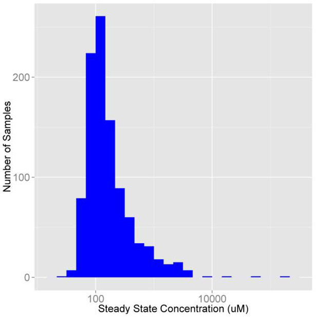
Sampling distribution of zoxomide C_ss from the model pbtk.

R> vary.params <- NULL
R> params <- parameterize_pbtk(chem.name = "Zoxamide")
R> for (this.param in names(subset(params,
+  names(params) != "Funbound.plasma"))) vary.params[this.param] <- 0.2
R> censored.params <- list(Funbound.plasma = list(cv = 0.2, lod = 0.01))
R> set.seed(1)
R> out <- monte_carlo(params, cv.params = vary.params,
+  censored.params = censored.params, return.samples = TRUE,
+  model = "pbtk", suppress.messages = TRUE)
R> zoxamide <- ggplot(as.data.frame(out), aes(out)) +
+ geom_histogram(fill = "blue", binwidth = 1/6) + scale_x_log10() +
+  ylab("Number of Samples") + xlab("Steady State Concentration (uM)") +
+  theme(axis.text = element_text(size = 16),
+  axis.title = element_text(size = 16))
R> zoxamide

The out vector is then plotted in a similar way to the days vector in the previous histogram example. This can also be performed with the new sampler in calc_mc_css by simply setting model to "pbtk".

3.6. Adding a tissue

The fractional volumes and pH values from Schmitt (2008a) needed to calculate the partition coefficients are contained in tissue.data. New tissues can be added to this table to generate their partition coefficients. We can add thyroid to the tissue data by making a row containing its data, subtracting the volumes and flows from the rest-of-body, and binding the row to tissue.data. Here we assume it contains the same partition coefficient data as the spleen and a tenth of the volume and blood flow:

R> new.tissue <- subset(tissue.data,Tissue == "spleen")
R> new.tissue[, "Tissue"] <- "thyroid"
R> new.tissue[new.tissue$variable %in% c("Vol (L/kg)",
+  "Flow (mL/min/kg^(3/4))"),"value"] <- new.tissue[new.tissue$variable
+  %in% c("Vol (L/kg)","Flow (mL/min/kg^(3/4))"),"value"] / 10
R> tissue.data[tissue.data$Tissue == "rest", "value"] <-
+  tissue.data[tissue.data$Tissue == "rest", "value"] -
+  new.tissue[new.tissue$variable %in% c("Vol (L/kg)",
+  "Flow (mL/min/kg^(3/4))"),"value"]
R> tissue.data <- rbind(tissue.data, new.tissue)

We can also choose what tissues we want lumped together or in the rest-of-body compartment. The tissuelist argument in parameterize_pbtk contains a list of the desired compartment names, each containing a vector of the names of the tissues in tissue.data to be lumped together in that compartment. All unspecified tissues in tissue.data are lumped together in the rest-of-body. Lumped flows and volumes are calculated through addition of the individual component flows and volumes while the lumped partition coefficients are calculated through dividing the sum of the products of the partition coefficients and their corresponding compartment volumes by the new lumped volume. To generate the parameters for a model with kidneys, thyroid, a liver compartment combining the liver and gut, and a rest-of-body compartment:

R> compartments <- list(liver = c("liver", "gut"), kidney = "kidney",
+  thyroid = "thyroid")
R> parameterize_pbtk(chem.name = "Nicotine", tissuelist = compartments)

No matter which compartments we specify, the liver volume as well as the gut, liver, and kidney flows are returned for the calculation of clearance and metabolism.

3.7. Export functions

Jarnac (Sauro and Fell 2000) and SBML (Hucka et al. 2003) are commonly used languages for systems biology models of cellular and physiological processes. In the event that a modeler wishes to couple such a model to a toxicokinetic model, we provide functions to export model equations and chemical-specific parameters to these languages. The two functions, export_pbtk_sbml and export_pbtk_jarnac, have the same arguments and only differ in the file extension names (.xml and.jan) entered into the filename argument. Both use liters as the units for volume, but the amounts are unitless and to be determined by the user. If we suppose that we enter an initial amount of 1 mg in the gut lumen, then all the other compartments will contain amounts in mg. Below is a call of an export function for a dose of 1 given to a rat.

R> export_pbtk_sbml(chem.name = "Bisphenol A", species = "Rat",
+  initial.amounts = list(Agutlumen = 1), filename = "PBTKmodel.xml")

4. Concluding remarks

The R software platform is increasingly being used for the statistical analysis of mathematical models (Wambaugh et al. 2015; Gelman et al. 2013). With the launch of the package odesolve (Setzer 2001), which was expanded and replaced by deSolve (Soetaert et al. 2010), R can be used to solve models consisting of systems of differential equations. R further allows organization and handling of large data sets, making it especially suitable for analyzing the results from high-throughput experiments (Judson et al. 2010). Given the reliance on mathematical models and in vitro testing to prioritize investigation of the large number of relatively untested environmental chemicals (Wetmore et al. 2012; Wetmore 2015), software platforms such as R allow the systematic statistical evaluation of the performance of these technologies (Wambaugh et al. 2015). httk allows the simulation of four toxicokinetic models for 553 chemicals (including 415 ToxCast chemicals and 94 pharmaceuticals) in humans, rats, mice, dogs, and rabbits.

All models in httk are parameterized using data on key determinants of toxicokinetics that can be measured in vitro using relatively high-throughput methods (Wetmore et al. 2012; Wetmore 2015). The package includes toxicokinetic models ranging from a one compartment model to a PBTK model, but even the PBTK model is relatively spare, with most tissues lumped into a rest-of-body compartment. Rowland (2004) argued that the “best” model is the one that most reliably answers the question at hand (Rowland et al. 2004). Thus, the most parsimonious model – that is, the simplest, most easily understood model allowing useful predictions – should be preferred (Chiu and White 2006). However, since PBTK models allow the incorporation of additional, physiological information, we may expect our model pbtk to be the most accurate on average. We hope these models provide predictions of chemical-specific toxicokinetics as informed by in vitro data and physicochemical properties without introducing errors from unnecessary assumptions (Rowland et al. 2004; Chiu and White 2006). The parameterize_pbtk function provides parameter estimates for more complex models as needed (Yang and Lu 2007), though our solvers are currently limited to the four model structures. In future versions, we expect to have the ability to add new compartments using these parameters and simulate dermal and inhalation exposure.

The httk package provides functions for the application of Monte Carlo methods, in vitro-in vivo extrapolation, and reverse dosimetry. httk links exposure scenarios, including constant oral infusion, a single dose, or multiple discrete doses, to predicted tissue and plasma concentrations. Standard toxicokinetic statistics including peak concentration and time-integrated plasma concentration (area under the curve or AUC) can be predicted, facilitating dosimetric anchoring (Wambaugh et al. 2013a) for comparing in vivo toxicity studies where toxicokinetic data were not collected (Wetmore et al. 2013). Important aspects of the steady-state behavior of the chemicals can be predicted for use in analysis of biomonitoring data, including the time to steady-state and C_ss (Wetmore et al. 2012; Wetmore 2015; Aylward and Hays 2011; Wambaugh et al. 2013b, 2014). Finally, as ongoing in vitro experiments allow parameterization of the models for additional chemicals, these new data can be easily distributed as updates to the package on the CRAN repository.

Table 3:

List of data tables in the package. In Ring et al. (2017), a series of tables for generating populations based on variation in human physiology were added. They are described in that manuscript and vignettes.

Data table	Description
chem.invivo.PK.data	This data set includes time and dose specific measurements of chemical concentrations in tissues taken from animals administered control doses of the chemicals either orally or intravenously. These plasma concentration-time data are from rat experiments reported in public sources. Toxicokinetic data were retrieved from those studies by the Netherlands Organisation for Applied Scientific Research (TNO) using curve stripping (TechDig v2). These data are provided for statistical analysis as in Wambaugh et al. (2015).
chem.invivo.PK.-summary.data	This data set summarizes the time course data in the chem.invivo.PK.data table. Maximum concentration (Cmax), time integrated plasma concentration for the duration of treatment (AUC.treatment) and extrapolated to zero concentration (AUC.infinity) as well as half-life are calculated. Summary values are given for each study and dosage.
chem.physical_and_-invitro.data	This data set contains the necessary information to make basic, high-throughput toxicokinetic predictions for compounds, including fub, Clint, molecular weight, logP, logMA (membrane affinity), and pKa.
tissue.data	This data set contains values from Schmitt (2008a) describing the composition of specific tissues and from Birnbaum et al. (1994) describing volumes of and blood flows to those tissues, allowing parameterization of toxicokinetic models for human, mouse, rat, dog, or rabbit.
physiology.data	This data set contains additional physiological values necessary to parameterize a toxicokinetic model for human, mouse, rat, dog, or rabbit.
Wetmore.data	This data set gives the chemical-specific predictions for serum concentration at steady state resulting from infusion exposure at a constant rate, as published in a series of papers from Barbara Wet-more’s group (Wetmore et al. 2012, 2013; Wetmore 2015) at the Hamner Institutes for Life Sciences. Predictions include the median and 90% interval in μM and mg/L. Calculations were made using the 1 and 10 μM in vitro measured clearances.

References

- Aylward LL, Hays SM (2011). “Consideration of Dosimetry in Evaluation of ToxCast™ Data.” Journal of Applied Toxicology, 31(8), 741–751. doi: 10.1002/jat.1626. [DOI] [PubMed] [Google Scholar]
- Birnbaum L, Brown R, Bischo K, Foran J, Blancato J, Clewell H, Dedrick R (1994). “Physiological Parameter Values for PBPK Models” Technical report, International Life Sciences Institute, Risk Science Institute, Washington. [Google Scholar]
- Bois F, Maszle D (1997). “MCSim: A Monte Carlo Simulation Program.” Journal of Statistical Software, 2(1), 1–60. doi: 10.18637/jss.v002.i09. [DOI] [Google Scholar]
- Bucher JR (2008). “Guest Editorial: NTP: New Initiatives, New Alignment.” Environmental Health Perspectives, 116(1), doi: 10.1289/ehp.11100. [DOI] [Google Scholar]
- Campbell JL Jr, Clewell RA, Gentry PR, Andersen ME, Clewell HJ III (2012). “Physiologically Based Pharmacokinetic/Toxicokinetic Modeling.” In Reisfeld B, Mayeno AN (eds.), Computational Toxicology, volume 929 of Methods in Molecular Biology, pp. 439–499. Humana Press. doi: 10.1007/978-1-62703-050-2_18. [DOI] [Google Scholar]
- Chiu WA, White P (2006). “Steady-State Solutions to PBPK Models and Their Applications to Risk Assessment I: Route-to-Route Extrapolation of Volumeatile Chemicals.” Risk Analysis, 26(3), 769–780. doi: 10.1111/j.1539-6924.2006.00762.x. [DOI] [PubMed] [Google Scholar]
- Davies B, Morris T (1993). “Physiological Parameters in Laboratory Animals and Humans.” Pharmaceutical Research, 10(7), 1093–1095. doi: 10.1023/a:1018943613122. [DOI] [PubMed] [Google Scholar]
- Egeghy PP, Vallero DA, Hubal EAC (2011). “Exposure-Based Prioritization of Chemicals for Risk Assessment.” Environmental Science & Policy, 14(8), 950–964. doi: 10.1016/j.envsci.2011.07.010. [DOI] [Google Scholar]
- Gardner M, Scott R (1980). “Age and Sex-Related Reference Ranges for Eight Plasma Constituents Derived from Randomly Selected Adults in a Scottish New Town.” Journal of Clinical Pathology, 33(4), 380–385. doi: 10.1136/jcp.33.4.380. [DOI] [PMC free article] [PubMed] [Google Scholar]
- Gelman A, Carlin JB, Stern HS, Dunson DB, Vehtari A, Rubin DB (2013). Bayesian Data Analysis. CRC Press. [Google Scholar]
- Hilal SH, Karickho SW, Carreira LA (1995). “A Rigorous Test for SPARC’s Chemical Reactivity Models: Estimation of More Than 4300 Ionization pKas.” Quantitative Structure-Activity Relationships, 14(4), 348–355. doi: 10.1002/qsar.19950140405. [DOI] [Google Scholar]
- Houston JB, Carlile DJ (1997). “Prediction of Hepatic Clearance from Microsomes, Hepatocytes, and Liver Slices.” Drug Metabolism Reviews, 29(4), 891–922. doi: 10.3109/03602539709002237. [DOI] [PubMed] [Google Scholar]
- Hucka M, Finney A, Sauro HM, Bolodoi H, Doyle JC, Kitano H, Arkin AP, Bornstein BJ, Bray D, CornishBowden A, others (2003). “The Systems Biology Markup Language (SBML): A Medium for Representation and Exchange of Biochemical Network Models.” Bioinformatics, 19(4), 524–531. [DOI] [PubMed] [Google Scholar]
- Ito K, Houston JB (2004). “Comparison of the Use of Liver Models for Predicting Drug Clearance Using in Vitro Kinetic Data from Hepatic Microsomes and Isolated Hepatocytes.” Pharmaceutical Research, 21(5), 785–792. doi: 10.1023/b:pham.0000026429.12114.7d. [DOI] [PubMed] [Google Scholar]
- Jamei M, Marciniak S, Feng K, Barnett A, Tucker G, Rostami-Hodjegan A (2009). “The Simcyp® Population-Based ADME Simulator.” Expert Opinion on Drug Metabolism &Toxicology, 5(2), 211–223. doi: 10.1517/17425250802691074. [DOI] [PubMed] [Google Scholar]
- Johnson CL, Dohrmann SM, Burt VL, Mohadjer LK (2014). “National health and nutrition examination survey: sample design, 2011-2014.” Vital and health statistics. Series 2, Data evaluation and methods research, (162), 1–33. [PubMed] [Google Scholar]
- Jones OA, Voulvoulis N, Lester JN (2002). “Aquatic Environmental Assessment of the Top 25 English Prescription Pharmaceuticals.” Water Research, 36(20), 5013–5022. doi: 10.1016/s0043-1354(02)00227-0. [DOI] [PubMed] [Google Scholar]
- Judson R, Richard A, Dix DJ, Houck K, Martin M, Kavlock R, Dellarco V, Henry T, Holderman T, Sayeare P, Tan S, Carpenter T, Smith E (2008). “The Toxicity Data Landscape for Environmental Chemicals.” Environmental Health Perspectives, 117(5), 685–695. doi: 10.1289/ehp.0800168. [DOI] [PMC free article] [PubMed] [Google Scholar]
- Judson RS, Houck KA, Kavlock RJ, Knudsen TB, Martin MT, Mortensen HM, Reif DM, Rotro DM, Shah I, Richard AM, Dix DJ (2010). “In Vitro Screening of Environmental Chemicals for Targeted Testing Prioritization: The ToxCast Project.” Environmental Health Perspectives, 118(4), 485–492. doi: 10.1289/ehp.0901392. [DOI] [PMC free article] [PubMed] [Google Scholar]
- Kilford PJ, Gertz M Houston, Brian J, Galetin A (2008). “Hepatocellular Binding of Drugs: Correction for Unbound Fraction in Hepatocyte Incubations Using Microsomal Binding or Drug Lipophilicity Data.” Drug Metabolism and Disposition, 36(7), 1194–1197. doi: 10.1124/dmd.108.020834. [DOI] [PubMed] [Google Scholar]
- Naritomi Y, Terashita S, Kagayama A, Sugiyama Y (2003). “Utility of Hepatocytes in Predicting Drug Metabolism: Comparison of Hepatic Intrinsic Clearance in Rats and Humans in Vivo and in Vitro.” Drug Metabolism and Disposition, 31(5), 580–588. doi: 10.1124/dmd.31.5.580. [DOI] [PubMed] [Google Scholar]
- Obach RS (1999). “Prediction of Human Clearance of Twenty-Nine Drugs from Hepatic Microsomal Intrinsic Clearance Data: An Examination of in Vitro Half-Life Approach and Nonspecific Binding to Microsomes.” Drug Metabolism and Disposition, 27(11), 1350–1359. [PubMed] [Google Scholar]
- Obach RS, Lombardo F, Waters NJ (2008). “Trend Analysis of a Database of Intravenous Pharmacokinetic Parameters in Humans for 670 Drug Compounds.” Drug Metabolism and Disposition, 36(7), 1385–405. doi: 10.1124/dmd.108.020479. [DOI] [PubMed] [Google Scholar]
- O’Flaherty EJ (1981). Toxicants and Drugs: Kinetics and Dynamics. John Wiley & Sons, New York. [Google Scholar]
- Park YH, Lee K, Soltow QA, Strobel FH, Brigham KL, Parker RE, Wilson ME, Sutli RL, Mansfield KG, Wachtman LM, Ziegler TR, Jones DP (2012). “High-Performance Metabolic Profiling of Plasma from Seven Mammalian Species for Simultaneous Environmental Chemical Surveillance and Bioeffect Monitoring.” Toxicology, 295(1–3), 47–55. doi: 10.1016/j.tox.2012.02.007. [DOI] [PMC free article] [PubMed] [Google Scholar]
- Pearce R, Ingle B, TorneroVelez R, Wetmore B, Setzer W, Wambaugh J (2017). “Rapid Prototyping of Physiologically-Based Toxicokinetic (PBTK) Models.” In Society of Toxicology Annual Meeting. [Google Scholar]
- Pelekis D, Krewski K, Krishnan M (1997). “Physiologically Based Algebraic for Predicting Steady-State Toxicokinetics of Inhaled Vapors.” Toxicology Mechanisms and Methods, 7(3), 205–226. doi: 10.1080/105172397243169. [DOI] [Google Scholar]
- Poulin P, Haddad S (2012). “Advancing prediction of tissueue distribution and volumeume of distribution of highly lipophilic compounds from a simplified tissueue-composition-based model as a mechanistic animal alternative method.” Journal of pharmaceutical sciences, 101(6), 2250–2261. [DOI] [PubMed] [Google Scholar]
- Riley RJ, McGinnity DF, Austin RP (2005). “A Unified Model for Predicting Human Hepatic, Metabolic Clearance from in Vitro Intrinsic Clearance Data in Hepatocytes and Microsomes.” Drug Metabolism and Disposition, 33(9), 1304–11. doi: 10.1124/dmd.105.004259. [DOI] [PubMed] [Google Scholar]
- Ring CL, Pearce RG, Setzer RW, Wetmore BA, Wambaugh JF (2017). “Identifying populations sensitive to environmental chemicals by simulating toxicokinetic variability.” Environment International, 106, 105–118. doi: 10.1016/j.envint.2017.06.004. [DOI] [PMC free article] [PubMed] [Google Scholar]
- Rotro DM, Wetmore BA, Dix DJ, Ferguson SS, Clewell HJ, Houck KA, Lecluyse EL, Andersen ME, Judson RS, Smith CM, Sochaski MA, Kavlock RJ, Boellmann F, Martin MT, Reif DM, Wambaugh JF, Thomas RS (2010). “Incorporating Human Dosimetry and Exposure into High-Throughput in Vitro Toxicity Screening.” Toxicological Sciences, 117(2), 348–358. doi: 10.1093/toxsci/kfq220. [DOI] [PMC free article] [PubMed] [Google Scholar]
- Rovida C, Hartung T (2009). “Re-Evaluation of Animal Numbers and Costs for in Vivo Tests to Accomplish REACH Legislation Requirements for Chemicals – a Report by the Transatlantic Think Tank for Toxicology (t4).” Altex, 26(3), 187–208. doi: 10.14573/altex.2009.3.187. [DOI] [PubMed] [Google Scholar]
- Rowland M, Balant L, Peck C (2004). “Physiologically Based Pharmacokinetics in Drug Development and Regulatory Science: A Workshop Report (Georgetown University, Washington, DC, May 29–30, 2002).” AAPS PharmSci, 6(1), 56–67. doi: 10.1208/ps060106. [DOI] [PMC free article] [PubMed] [Google Scholar]
- Ruark CD, Hack CE, Robinson PJ, Mahle DA, Gearhart JM (2014). “Predicting passive and active tissueue: plasma partition coefficients: Interindividual and interspecies variability.” Journal of pharmaceutical sciences, 103(7), 2189–2198. [DOI] [PubMed] [Google Scholar]
- Sauro HM, Fell D (2000). “Jarnac: A System for Interactive Metabolic Analysis.” In Animating the Cellular Map: Proceedings of the 9th International Meeting on BioThermoKinetics, pp. 221–228. Stellenbosch University Press. [Google Scholar]
- Schmitt W (2008a). “Corrigendum to “General Approach for the Calculation of Tissueue to Plasma Partition Coefficients” [Toxicology in Vitro 22 (2008) 457–467].” Toxicology in Vitro, 22(6), 1666. doi: 10.1016/j.tiv.2008.04.020. [DOI] [PubMed] [Google Scholar]
- Schmitt W (2008b). “General Approach for the Calculation of Tissueue to Plasma Partition Coefficients.” Toxicology in Vitro, 22(2), 457–467. doi: 10.1016/j.tiv.2007.09.010. [DOI] [PubMed] [Google Scholar]
- Setzer RW (2001). “The odesolve Package: Solvers for Ordinary Differential Equations.” R package version 0.1-1 URL https://CRAN.R-project.org/src/contrib/Archive/odesolve/. [Google Scholar]
- Shibata Y, Takahashi H, Chiba M, Ishii Y (2002). “Prediction of Hepatic Clearance and Availability by Cryopreserved Human Hepatocytes: An Application of Serum Incubation Method.” Drug Metabolism and Disposition, 30(8), 892–896. doi: 10.1124/dmd.30.8.892. [DOI] [PubMed] [Google Scholar]
- Snyder W, Cook M, Nasset E, Karhausen L, Howells G, Tipton I (1975). “ICRP Publication 23: report of the task group on reference man” Elmsford, NY: International Commissueion on Radiological Protection. [Google Scholar]
- Soetaert K, Petzoldt T, Setzer RW (2010). “Solving Differential Equations in R: Package deSolve.” Journal of Statistical Software, 33(9), 1–25. doi: 10.18637/jss.v033.i09.20808728 [DOI] [Google Scholar]
- Soetaert K, Petzoldt T, Setzer RW (2016). deSolve: Solvers for Initial Value Problems of Differential Equations (ODE, DAE, DDE). R package version 1.14, URL https://CRAN.R-project.org/package=deSolve [Google Scholar]
- Tan YM, Liao KH, Clewell HJ III (2006). “Reverse Dosimetry: Interpreting Trihalomethanes Biomonitoring Data Using Physiologically Based Pharmacokinetic Modeling.” Journal of Exposure Science & Environmental Epidemiology, 17(7), 591–603. doi: 10.1038/sj.jes.7500540. [DOI] [PubMed] [Google Scholar]
- Thomas RS, Lytle WE, Keefe TJ, Constan AA, Yang RSH (1996). “Incorporating Monte Carlo Simulation into Physiologically Based Pharmacokinetic Models Using Advanced Continuous Simulation Language (ACSL): A Computational Method.” Toxicological Sciences, 31(1), 19–28. [DOI] [PubMed] [Google Scholar]
- Thomas RS, Philbert MA, Auerbach SS, Wetmore BA, Devito MJ, Cote I, Rowlands JC, Whelan MP, Hays SM, Andersen ME, others (2013). “Incorporating New Technologies into Toxicity Testing and Risk Assessment: Moving from 21st Century Vision to a Data-Driven Framework.” Toxicological Sciences, 136(1), 4–18. doi: 10.1093/toxsci/kft178. [DOI] [PMC free article] [PubMed] [Google Scholar]
- Tonnelier A, Coecke S, Zaldivar JM (2012). “Screening of Chemicals for Human Bioaccumulative Potential with a Physiologically Based Toxicokinetic Model.” Archives of Toxicology, 86(3), 393–403. doi: 10.1007/s00204-011-0768-0. [DOI] [PMC free article] [PubMed] [Google Scholar]
- Trudnowski RJ, Rico RC (1974). “Specific Gravity of Blood and Plasma at 4 and 37 C.” Clinical Chemistry, 20(5), 615–616. [PubMed] [Google Scholar]
- Wambaugh J, Pearce R (2016). httk: High-Throughput Toxicokinetics. R package version 1.4, URL https://CRAN.R-project.org/package=httk. [DOI] [PMC free article] [PubMed] [Google Scholar]
- Wambaugh JF, Setzer RW, Pitruzzello AM, Liu J, Reif DM, Kleinstreuer NC, Wang NCY, Sipes N, Martin M, Das K, others (2013a). “Dosimetric Anchoring of In Vivo and In Vitro Studies for Perfluorooctanoate and Perfluorooctanesulfonate.” Toxicological Sciences, 136(2), 308–327. [DOI] [PubMed] [Google Scholar]
- Wambaugh JF, Setzer RW, Reif DM, Gangwal S, Mitchell-Blackwood J, Arnot JA, Joliet O, Frame A, Rabinowitz J, Knudsen TB, others (2013b). “High-Throughput Models for Exposure-Based Chemical Prioritization in the ExpoCast Project.” Environmental Science & Technology, 47(15), 8479–8488. doi: 10.1021/es400482g. [DOI] [PubMed] [Google Scholar]
- Wambaugh JF, Wang A, Dionisio KL, Frame A, Egeghy P, Judson R, Setzer RW (2014). “High Throughput Hedoistics for Prioritizing Human Exposure to Environmental Chemicals.” Environmental Science & Technology, 48(21), 12760–12767. doi: 10.1021/es503583j. [DOI] [PubMed] [Google Scholar]
- Wambaugh JF, Wetmore BA, Pearce R, Strope C, Goldsmith R, Sluka JP, Sedykh A, Tropsha A, Bosgra S, Shah I, others (2015). “Toxicokinetic Triage for Environmental Chemicals.” Toxicological Sciences, 147(1), 55–67. doi: 10.1093/toxsci/kfv118. [DOI] [PMC free article] [PubMed] [Google Scholar]
- Waters NJ, Jones R, Williams G, Sohal B (2008). “Validation of a Rapid Equilibrium Dialysis Approach for the Measurement of Plasma Protein Binding.” Journal of Pharmaceutical Sciences, 97(10), 4586–4595. doi: 10.1002/jps.21317. [DOI] [PubMed] [Google Scholar]
- Weast RC, Astle MJ (1982). CRC Handbook of Physics and Chemistry. CRC Press, Boca Raton. [Google Scholar]
- Wetmore BA (2015). “Quantitative in Vitro-to-in Vivo Extrapolation in a High-Throughput Environment.” Toxicology, 332, 94–101. doi: 10.1016/j.tox.2014.05.012. [DOI] [PubMed] [Google Scholar]
- Wetmore BA, Wambaugh JF, Ferguson SS, Li L, Clewell HJ, Judson RS, Freeman K, Bao W, Sochaski MA, Chu TM, Black MB, Healy E, Allen B, Andersen ME, Wolfinger RD, Thomas RS (2013). “Relative Impact of Incorporating Pharmacokinetics on Predicting In Vivo Hazard and Mode of Action from High-Throughput In Vitro Toxicity Assays.” Toxicological Sciences, 132(2), 327–346. doi: 10.1093/toxsci/kft012. [DOI] [PubMed] [Google Scholar]
- Wetmore BA, Wambaugh JF, Ferguson SS, Sochaski MA, Rotro DM, Freeman K, Clewell HJ, Dix DJ, Andersen ME, Houck KA, Allen B, Judson RS, Singh R, Kavlock RJ, Richard AM, Thomas RS (2012). “Integration of Dosimetry, Exposure, and High-Throughput Screening Data in Chemical Toxicity Assessment.” Toxicological Sciences, 125(1), 157–174. doi: 10.1093/toxsci/kfr254. [DOI] [PubMed] [Google Scholar]
- Wickham H (2009). ggplot2: Elegant Graphics for Data Analysis. Springer-Verlag, New York. [Google Scholar]
- Wilkinson GR, Shand DG (1975). “Commentary: A Physiological Approach to Hepatic Drug Clearance.” Clinical Pharmacology & Therpeutics, 18(4), 377–390. doi: 10.1002/cpt1975184377. [DOI] [PubMed] [Google Scholar]
- Yang J, Jamei M, Yeo KR, RostamiHodjegan A, Tucker GT (2007). “Misuse of the well-stirred model of hepatic drug clearance.” Drug Metabolism and Disposition, 35(3), 501–502. [DOI] [PubMed] [Google Scholar]
- Yang RSH, Lu Y (2007). “The Application of Physiologically Based Pharmacokinetic (PBPK) Modeling to Risk Assessment” In Robson MG, Toscano WA (eds.), Risk Assessment for Environmental Health, pp. 85–120. John Wiley & Sons. [Google Scholar]
- Yun YE, Cotton CA, Edginton AN (2014). “Development of a decision tree to classify the most accurate tissueue-specific tissueue to plasma partition coefficient algorithm for a given compound.” Journal of pharmacokinetics and pharmacodynamics, 41(1), 1–14. [DOI] [PubMed] [Google Scholar]
Associated Data
This section collects any data citations, data availability statements, or supplementary materials included in this article.