Abstract
Epilepsy is a neurological disorder that can negatively affect the visual, audial and motor functions of the human brain. Statistical analysis of neurophysiological recordings, such as electroencephalogram (EEG), facilitates the understanding and diagnosis of epileptic seizures. Standard statistical methods, however, do not account for topological features embedded in EEG signals. In the current study, we propose a persistent homology (PH) procedure to analyze single-trial EEG signals. The procedure denoises signals with a weighted Fourier series (WFS), and tests for topological difference between the denoised signals with a permutation test based on their PH features persistence landscapes (PL). Simulation studies show that the test effectively identifies topological difference and invariance between two signals. In an application to a single-trial multichannel seizure EEG dataset, our proposed PH procedure was able to identify the left temporal region to consistently show topological invariance, suggesting that the PH features of the Fourier decomposition during seizure is similar to the process before seizure. This finding is important because it could not be identified from a mere visual inspection of the EEG data and was in fact missed by earlier analyses of the same dataset.
Keywords and phrases: persistence landscape, persistent homology, weighted Fourier series, electroencephalogram, epilepsy
1. Introduction
Epilepsy is a neurological problem that can negatively affect the visual, audial and motor abilities of a patient. During an epileptic seizure attack, the patient may experience idiosyncratic symptoms ranging from visual hallucinations to sense of disassociation (Bancaud et al., 1994; Fried, 1997). Findings by the World Health Organization (WHO) indicate that approximately nine in one thousand people around the world suffered from epilepsy in 1998 (WHO, 2005). The Centers for Disease Control and Prevention (CDC) have recently reported that an estimated one percent of adults in the United States currently suffer from active epilepsy (Kobau et al., 2012). Researchers are pursuing all possible avenues to gain a better understanding and management of the disease. One key area of research tries to understand the epileptogenic zone, i.e the set of brain sites involved in the generation of seizures, particularly for the purpose of epilepsy surgery as the surgical procedure aims to remove the epileptogenic zone. However, high failure rate in epilepsy surgery suggests that epileptogenicity remains elusive (Bartolomei, Chauvel and Wendling, 2008). It is our goal in this paper to develop a rigorous procedure to better understand the epileptogenic zone based on electrophysiological data from an epilepsy patient.
Electroencephalogram (EEG) is an important electrophysiological modality for understanding the function and dysfunction of the brain. It is popular in studying epileptic seizures because of its non-invasive procedure and high temporal resolution. EEG signals are synchronous discharges from cerebral neurons detected by electrodes placed on the scalp or intracranially implanted in the patient. Epileptic seizure is associated with abnormality in EEG recordings and is characterized by brief and episodic neuronal synchronous discharges with dramatically increased amplitude. The anomalous synchrony in seizure attacks may occur as a partial seizure which is seen only in a few local channels of the EEG signal, or as a generalized seizure which is observed in every channel of the EEG signal. State-of-the-art statistical methods have been developed over the past decades to study the patterns of the nonlinear electrical signals in epileptic seizures (Donoho, Mallat and von Sachs, 1998; Mitra and Pesaran, 1999; Ombao et al., 2001; Ombao, von Sachs and Guo, 2005). In the medical literature, more accessible methods have been developed for the purpose of understanding epileptogenicity with EEG signals observed inbetween and during seizure attacks (Martinerie et al., 1998; McSharry, Smith and Tarassenko, 2003; Bartolomei, Chauvel and Wendling, 2008). These methods tend to utilize transformed information, such as time-frequency and phase space, of the seizure EEGs. Methods that utilizes EEG information in the time domain are few and far between. The local variance method, where variances of signal amplitude are computed in a moving window across time, often serve as a baseline. The simplistic approach has shown to be more effective in some cases than methods utilizing transformed information (Martinerie et al., 1998; McSharry, Smith and Tarassenko, 2003; Mohseni, Maghsoudi and Shamsollahi, 2006).
One aspect of univariate EEGs that has rarely been explored is topological information in the signals. Since differences in amplitude and frequency do not necessarily correspond to topological difference in EEG signals, we are motivated to develop a rigorous procedure based on spectra-temporal information of the signals that is invariant to the usual signal difference. A promising exploratory approach is the topological data analysis (TDA), an umbrella term for various topological techniques utilized to analyze scientific data (Carlsson, 2009). A key TDA technique is persistent homology (PH) developed by (Edelsbrunner, Letscher and Zomorodian, 2002). PH tracks changes in topological features of of EEG data based on the content of oscillations (i.e., spectrum) across multiple resolutions and dimensions. PH on the EEG signal summarizes the evolution of the connected components (based on the Fourier coefficients of the signal). PH descriptors such as the barcode and persistence diagram (PD) keep track of the birth and death times of connected components as they appear and disappear in the sublevel set when the sublevel threshold λ increases. The parameter λ is analogous to but more general than the thresholding level in multi-resolution wavelet analysis (Chung et al., 2014).
PH has been applied to a wide range of data: Sousbie, Pichon and Kawahara (2011) invoked the PH idea for scale-free and parameter-free identification of the voids, walls, filaments, clusters and their configuration within the cosmic web; Petri et al. (2013) deployed PH in studying a number of weighted complex networks: US air passenger networks, online messages and forums, gene networks, Twitter, and co-authorship networks; Ahmed, Fasy and Wenk (2014) utilized a localized version of PH to compare the intrinsic structures of two road networks. Existing PH applications on imaging data have mostly focused on static multivariate random samples, typically from positron emission tomography (PET) and magnetic resonance imaging (MRI) studies (Gamble and Heo, 2010; Lee et al., 2011; ?). A popular approach is to model the data as a network or graph based on sites on the brain and join two sites when the distance between them exceeds a certain threshold λ. This approach has also been applied to EEG functional networks in a mouse model of depression (Khalid et al., 2014). It is a challenge to perform inference on barcode and PD directly due to theoretical and practical reasons to be discussed in Section 3. An alternative PH descriptor called persistence landscape (PL) that builds landscape-like features was proposed by (Bubenik, 2015) with a rigorous statistical framework. Yet its development has mostly been theoretical and biomedical applications are sporadic.
We summarize our contributions in this paper.
The proposed TDA framework is the first method to incorporate persistence landscape in the analysis of connected components of univariate EEG signals based on the Fourier coefficients.
We claim topological invariance as a “signal”. Using the proposed TDA method, we identified topological invariance before and during seizure of signals around the seizure location, which was not previously discovered by other methods that used the same data (e.g., SLEX methods in Ombao et al. (2001, 2005)). Our simulation studies show that the TDA approach is robust to topologically invariant transformations such as translation, amplitude and frequency scaling. It is also sensitive to topology-destroying transformations such as tearing.
In Section 2, we provide the necessary background on PH and motivate its application on EEG data. In Section 3, we present our methods for fitting and resampling thresholded WFS of single-trial multichannel EEG signals, and for inference on the PLs of the resampled thresholded WFS before and during a seizure attack. Sections 4 and 5 are designated for simulation studies and data application. The results are promising and provide new insight on epileptogenicity through single-trial multichannel EEG signals.
2. Preliminary on persistent homology
Our goal is to utilize topological features in comparing EEG signals before and during a seizure attack. To achieve our goal, we shall first explain the basic ideas about topological features characterized by PH in point-cloud data and univariate functional signals. Note that we only discuss the aspects of PH relevant to our aim. A comprehensive introduction to PH can be found in (Edelsbrunner and Harer, 2010).
In algebraic topology, the connectedness of a topological space is summarized by its homology groups and corresponding Betti numbers βi for i = 0, 1, 2, … (up to the dimension of the underlying space). In a three-dimensional space, β0, β1 and β2 are the numbers of connected components, tunnels and voids respectively. Algorithmic computation of Betti numbers is efficient for certain topological spaces such as simplicial complexes.
A simplicial complex is a combinatorial structure of simplices. A p-simplex Δ is the convex hull of p + 1 affinely independent points
Each point υi is a 0-simplex, a pair of points υi and υj joined by an edge is a 1-simplex, a triangle formed by three points υi, υj, υk joined by three edges is a 2-simplex, and a tetrahedron formed by 4 triangles is a 3-simplex (Figure 1). A face of Δ is the convex hull of a nonempty subset of {υ0, υ1, …, υp}. For instance, the faces of a tetrahedron are its points, edges and triangles. A simplicial complex K is constructed by attaching simplices with respect to a certain set of rules: a simplex joins K when all of its faces have joined and the intersection of two simplices in the complex K must be a face to each of the simplices.
Fig 1.
Simplices in ℝ3; one point υ0 is a 0-simplex, a pair of points υ0 and υ1 joined by an edge is a 1-simplex, a triangle formed by three points υ0, υ1, υ2 joined by three edges is a 2-simplex, and a tetrahedron formed by 4 triangles is a 3-simplex.
Given a dataset of points S = {xi} in a topological space X ⊂ ℝd, we are interested in the extent to which the homology of X can be inferred from the simplicial complex built on S. The idea is to attach (or equivalently delete) the simplices in such a way that the resulting simplicial complex reveals the homology of the data. The most common simplicial complex is the Vietoris-Rips complex (or Rips complex for short). The p-simplices in the Rips complex correspond to p + 1 points of {xi} pairwise distance exceeding a certain threshold λ. By varying λ, the simplicial complex changes. We can keep track of the birth and death times of holes in the changing sequence of complexes, or filtration, with intervals or bars over increasing λ. A long bar indicates a hole that persists over a long range of parameter values and therefore corresponds to a large scale topological feature in X, whereas short intervals correspond to noise or inadequate sampling (Carlsson, 2009). This is the idea behind persistent homology (PH), a novel computational topology method introduced by Edelsbrunner, Letscher and Zomorodian (2002).
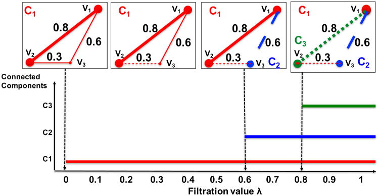
The intuition behind PH can be illustrated by a simple example of Rips filtration constructed on three-point cloud data in Figure 2. The filtration starts out with a 2-simplex, which we call connected component 1 (CI). We vary a threshold λ - the filtration value - from 0 and upward. When λ reaches 0.3 - the smallest edge length - in the 2-simplex, the edge that connects the points υ2 and υ3 is deleted. But the deletion does not affect the connectedness of the 2-simplex. Only when we hit λ = 0.6 that υ3 breaks out a separate connected component (C2) from CI. The 2-component structure remains until we reach λ = 0.8 when the vertex υ1 becomes a separate connected component (C3) from CI and C2. There are no more connected components in the filtration as the 2-simplex only has three points. The lower part of Figure 2 shows the collection of bars, or barcode, corresponding to the connected structure in the process, or filtration. The bars represent the birth and death times of the connected components. Since λ varies monotonely, deleted edges can no longer come back to the filtration to connect components already separated. Therefore the death ends of the bars will hold out to infinity. Thinning out or adding on the edges result in equivalent filtrations.
Fig 2.
An example of Rips filtration and its corresponding barcode.
Persistent homology on functional data
In application, the Rips filtration has been popular in network modeling on brain imaging data (Lee et al., 2011; ?). It is useful for extracting topological information in point cloud data modeled as a graph. The method, however, is not applicable in the context of one-dimensional functional data. The only topological information of a one-dimensional function g : 𝒳 ⊂ ℝ → ℝ is the connected components in its sublevel set
for some λ ∈ ℝ. The birth and death of the connected components as the threshold λ varies is characterized by the pairing of local minimums and maximums called the Morse Filtration (?Chung, Bubenik and Kim, 2009; Bubenik et al., 2010).
To see this, consider the example of a mixture distribution g : 𝒳 ⊂ ℝ → [0, ∞) truncated on 𝒳 = [−5, 10]:
| (1) |
where wi = 1/4 and
with μ1 = −2, σ1 = 1; μ2 = 2, σ2 = 1.5; μ3 = 5.5, σ3 = 1; μ4 = 8, σ4 = 1. Figure 3 illustrates how local minimums and maximums characterize the birth and death of connected components in the sublevel set of (1). A horizontal line of reference indicating the threshold λ moves from the minimum value of the function and up. Before the line hits the point A, the sublevel set of the function is empty except for the boundaries. After the line touches A, the sublevel set becomes a line segment on the x-axis underneath A that grows as the reference line keeps moving upward. Another line segment under B joins the sublevel set when the reference line hits point B. The two line segments join up when the reference line reaches point C. According to the Elder Rule (Edelsbrunner and Harer, 2010), we pair point B with point C and leave point A with the oldest line segment in the sublevel set to be paired with a later point. As we reach point D, a new line segment emerges in the sublevel set and is annihilated. The next point reached is E, where the left boundary merges with the big component joined by line segments A and B. When the reference line reaches the point F, the line segment created at D is merged with the right boundary. So we pair D with F. Lastly, the two big components are joined as one at the point G and we pair the minimum value of the function with G. The birth and death times of the all connected components in the sublevel set are encoded in the PD.
Fig 3.
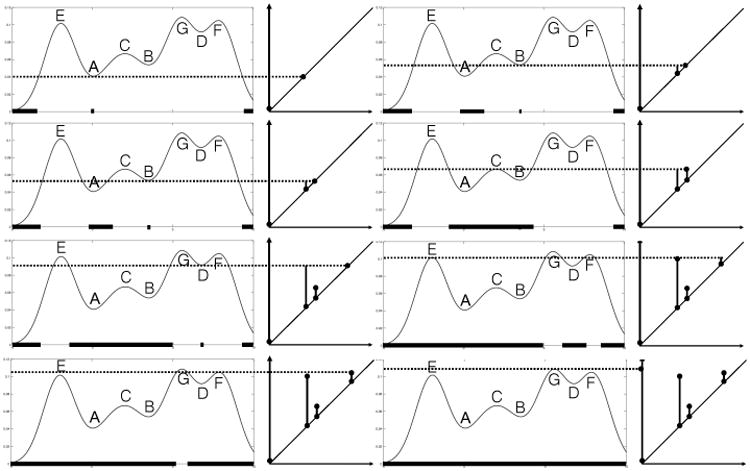
The evolution of connected components in the sublevel set of the mixture distribution (1), and corresponding persistence diagram.
In the subsequent sections, we utilize the PH characterization of sublevel-set connectedness to study the topological difference between EEG signals.
3. Methods
In this section, we first introduce a denoising procedure for a univariate EEG signal. We then introduce the mathematical detail on PL and how to construct it on a denoised signal. Last we propose a PL-based permutation test for studying topology of seizure EEG signals.
3.1. Signal denoising by thresholded weighted Fourier series
Algorithms processing raw data may pick up more on error than on signal, particularly in the analysis of connected component evolution (Bendich et al., 2016). To stabilize the subsequent topological analysis, we first denoise a raw EEG signal by estimating μ in the model:
| (2) |
where f is the raw EEG signal assumed to come from the space of square integrable functions on ℝ equipped with the inner product
with respect to the Lebesgue measure ℓ. The additive model (2) is the most fundamental and flexible scientific model for a stochastic process. We can impose different structures on the noise component for varying levels of model complexity. We require the underlying functional μ(t) to be continuous but not necessarily smooth.
Our denoising approach first estimates μ(t) by a weighted Fourier representation. We can describe the human brain signals with the WFS because EEGs are often considered as superpositions of sine and cosine waveforms with varying amplitudes, and the weighting governs the relative weights of the high-frequency components to the low-frequency ones. On a deeper level, the weighted Fourier approach is motivated by the connection between kernel estimation and heat diffusion equation. The popular Gaussian kernel estimator is noted to be equivalent to the solution of a Fourier heat equation (Chaudhuri and Marron, 2000). Botev, Grotowski and Kroese (2010) also note that a more general heat diffusion equation generates a large class of kernel estimators with desirable statistical properties. Here we utilize the series solution to the linear diffusion equation
| (3) |
By treating the observed signal f as the initial condition of the diffusion equation:
and imposing the periodic boundary conditions
on (3), we are able to obtain a closed-form weighted Fourier series (WFS) estimate (Chung et al., 2007, 2014) for the signal f:
| (4) |
with the eigenvalues γj = (jπ/T)2 for j ≥ 1, the Fourier coefficients
and the basis functions
| (5) |
| (6) |
The degree-k representation of (4) is
| (7) |
where the degree k decides the highest frequency [k/T] to be included in the representation (e.g. 100Hz for k = 499 and T = 5), and the relative weights of the high frequency components to the low frequency components is governed by the parameter σ.
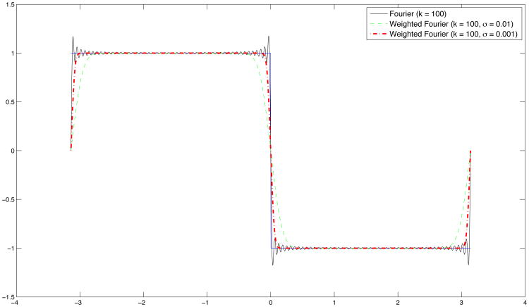
WFS effectively reduces the Gibbs phenomenon in the FS estimation of data at discontinuities (Chung et al., 2014). Figure 4 shows FS and WFS in a simple example. The underlying function takes step values 1 and -1 on the intervals [−π, 0) and [0, π] respectively. All series estimation is based on the first 50 terms of finite approximation. The discontinuity at π and the two end-points cause the FS to overshoot, whereas the WFS is not affected in the same way.
Fig 4.
Gibbs phenomenon (ringing artifacts) is visible in the Fourier series expansion of a step function, whereas the weighted Fourier series approximation shows less visible artifacts.
In practice, some low-frequency components may not matter in the degree-k WFS estimator (7). So we only include sine or cosine waveform (even those that at high frequencies) in the representation if the corresponding amplitudes exceed some threshold. We borrow strength from wavelet thresholding (Donoho and Johnstone, 1994, 1995; Abramovich and Benjamini, 1996) to delete frequency components that are of lesser importance:
| (8) |
with
| (9) |
where Tu is the universal threshold
| (10) |
where n is the number of data points in each phase and s is the median of the absolute deviation (MAD) of the Fourier coefficients:
| (11) |
In summary, a univariate EEG signal is represented as superpositions of sinusoidal functions. Sinusoids corresponding to high-frequency oscillations and relatively lower contribution to the total variation in the signal are removed.
We fit the thresholded degree-k WFS estimator to the signals f1(t) and f2(t) before and during seizure (Phase 1 and 2):
| (12) |
| (13) |
where aij and bij are Fourier coefficients for Phase i, i = 1, 2:
| (14) |
and the index sets ℐi1 and ℐi2 contain the thresholded aij and bij:
| (15) |
where is the universal threshold for Phase i, i = 1, 2 with
3.2. Topological permutation test on single-trial seizure EEGs
Our goal is to compare the topological features of denoised single-trial EEG signals before and during seizure. It is essential to account for invariance in the topological comparison. To see this, consider a continuous mapping or transformation 𝒟 of a denoised EEG signal g(t) on −T ≤ t ≤ T:
As explained in Section 2, the topology of the sublevel set of a signal is characterized by the pairing of the local minima and maxima. The topology remains the same if the relative positions of the critical points remain intact up to scaling. Continuous transformations such as translation and scaling do not change the relative positions of the critical points in a signal - thus the invariance of sublevel-set topology. Tearing, on the other hand, destroys the topology in the sublevel set of the signal (Munkres, 1984).
We need a statistical test to stay robust under topological invariant transformations, and at the same time reasonably sensitive to tearing operations, where the resulting difference in the original and transformed signals is considered as true topological difference. Standard tests based on amplitude, frequency or time-frequency features of EEG signals may not serve the purpose as they do not account for topological features. We are thus motivated to develop a test based on PH features for topological comparison between single-trial EEG signals. Barcode and PD are the original descriptors developed to summarize equivalent PH features. PD has been shown to possess desirable properties such as Lipschitz stability with respect to the bottleneck distance (Cohen-Steiner, Edelsbrunner and Harer, 2007; Cohen-Steiner and Edelsbrunner, 2009). It was also shown in (Mileyko, Mukherjee and Harer, 2011) that the PDs under the Wasserstein distance form a Polish space -a complete and separable metric space. The mean and variance appropriate for the space are the so-called Fréchet mean and variance. The Fréchet mean, however, is not unique (Turner et al., 2014), rendering it a challenging statistical issue to perform inference on PDs directly. Notable PD applications in imaging studies also realize that inference on PD is by no means straightforward in practice (Chung, Bubenik and Kim, 2009; Gamble and Heo, 2010; Heo, Gamble and Kim, 2012).
An alternative PH descriptor PL was proposed by Bubenik (2015) for the purpose of statistical analysis. Given a bar (a, b) in a barcode with a ≤ b, we can define the piecewise linear bump function h(a,b) : ℝ → ℝ by
| (16) |
The geometric representation of the bump function (16) is a right-angled isosceles triangle with height equal to half of the base of the corresponding interval in the barcode. The PL of is the set of functions defined by
| (17) |
with νk(x) = 0 for k > N. Geometrically, νk is the k-th layer of the PL and traces the k-th outermost outline of the crossover triangles in the bump function. The landscape has value zero elsewhere. Figures 5 illustrates PL based on the example shown in Figure 3. The main technical advantage of PL is that, as a function on a separable Banach space, the theory (and results) of random variables can be applied (Bubenik, 2015; Chazal et al., 2014).
Fig 5.
Barcode and persistence landscape (PL) based on the example shown in Figure 3.
To compare the PLs
of two samples of signals, an existing parametric approach is to apply first a real-valued functional satisfying regularity conditions to the PLs (Bubenik, 2015). A two-sample z-test can then be built on the sample means of the functional satisfying asymptotic normality. The test is, however, not sensitive enough to difference between two sets of PLs. The alternative of applying the Hotelling's T2 test to a vector of functional difference between the individual layers of two sets of PLs improves on power but is insufficient when the PLs are translates of each other. Most importantly, in the case of single-trial seizure EEGs, the dataset does not contain multiple signals; we only observe two PLs
of the respective WFS (12) and (13) for Phases 1 and 2 of a seizure. Creating signal replicates with a resampling procedure requires additional work and justification on the covariance estimation of the corresponding PLs.
To overcome the limitations of existing parametric tests on PLs, we propose a PL-based permutation test for testing the topological difference between two WFS-denoised single-trial EEG signals. The permutation test is distribution-free and can be flexibly applied to individual or all layers of PLs without the restriction of a functional. Under the null hypothesis, we assume no topological difference between the two signals. That is, the spectral features and relative contribution of the different oscillations (averaged across the two signals) are identical. In order to create replicates from the single-trial signals for inference, we require a resampling step in our procedure. If we resample an EEG signal in the time domain (Politis, Romano and Wolf, 1999), it would destroy the topological structure in the sublevel set of the signal. It is also more complicated than a permutation approach in the frequency domain. Under the null hypothesis, the labels (Phase 1 and Phase 2) of the coefficients at each frequency can be interchanged. Hence, the procedure randomly exchanges the frequency components in the two signals, i.e., the Fourier coefficients in (14), to reconstruct two sets of signal replicates in the time domain by plugging resampled Fourier coefficients in (12) and (13). For each resample, we calculate the L2 distance between the PLs and of the two reconstructed WFS:
| (18) |
Note that N, the number of PL layers, is not a fixed number for all PLs. So when comparing two PLs, we take N to be the larger of the numbers of layers of two PLs. The landscape with the smaller number of layers is padded with zeros in the layers that it does not have in comparison with the other landscape.
Using the above permutation test, two phases are declared to be topologically invariant if the topological distance between the observed signals does not exceed that of the threshold in the distribution of topological distances in the resampled pairs of signals. In Section 4, we test out the performance of the proposed method with respect to simulated ground truth. In Section 5, we use the proposed permutation test to study how topological invariance manifests in and out of the epileptogenic zone in a single-trial seizure EEG dataset.
4. Simulations
Simulation studies are organized in two parts: performance of the frequency resampling approach and the topological permutation test against baseline methods. The two parts of simulations are independent in data generation and test procedure.
4.1. Performance of frequency resampling method
This set of simulations demonstrate that permutation of Fourier coefficients has acceptable false positive rate and power. We simulate two signals y1(t) and y2(t) for −5 ≤ t ≤ 5 via truncated WFS:
| (19) |
| (20) |
where
| (21) |
| (22) |
with and . We are interested in testing the equivalence of two WFS y1 and y2, which are equivalent if and only if all the coefficients are equivalent. This results in testing the hypothesis
we permute the cij and dij in pairs to obtain and and two corresponding resampled signals y1′(t) and y2′(t):
| (23) |
| (24) |
One way to measure the difference between two signals y1(t) and y2(t) (similarly y1′(t) and y2′(t)), −T ≤ t ≤ T, is the L2 distance
where we set T = 5. The p-value for each simulation is calculated as the proportion of the L2(y1′, y2′) that exceed L2(y1, y2). As a performance measure, we collect the p-values in 100 simulations and compute the percentages of those below 0.05 and 0.01. Due to different magnitudes of variance, we expect the percentages in Study 1 and Study 2 to be small and large respectively.
Study 1
In this setting, the noise components are generated with
for signals constructed at k = 99 and σ = 0. The percentages of p-values below 0.05 and 0.01 are both 1%.
Study 2
In this setting, the noise components are generated with
for signals constructed at k = 99 and σ = 0. The percentages of p-values below 0.05 and 0.01 are both 100%.
4.2. Performance of topological permutation test
The TDA procedure proposed in Section 3 is designated to discern underlying topological difference between two signals. It is also expected to have a low false positive rate and high power in detecting true topological difference. To measure the performance of the test, we compare it with two baseline methods on signals simulated with respect to different mathematical transformations.
Study 1. Topological invariance
The idea is to simulate two signals with the same underlying topologies. The topological identity at the presence of noise is expected to be recognized by the topological permutation test. We firs simulate a continuous function g(t) with unique critical points. The second signal is simulated in three settings with respect to concrete types of topological invariance transformations of g(t):
-
Translation:
-
Scaling amplitude:
for c > 1 (c < 1), the function is stretched (squeezed) in the amplitude.
-
Scaling frequency:
for ω < 1 (ω > 1), the function is stretched (squeezed) in the direction of t.
Shifting or scaling a functional signal in the horizontal (frequency) or vertical direction (amplitude) alter its geometry, but not its topology.
For each parameter setting of a study, 100 datasets are simulated. In each dataset, two blocks of signals are generated according to the topology-preserving transformations of a function. Independent noises are added to the signals. The null hypothesis of topological invariance is rejected in a simulation if the p-value was small. Percentages out of the 100 simulations are then computed for p-values below 0.05. Percentages below 5% are considered as good performance in robustness.
Study 1.1. Translation
We simulate four pairs of signals y1(t) and y2(t), 0 ≤ t ≤ 2π:
| (25) |
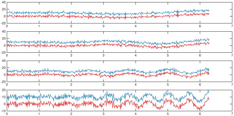
where ω takes on four values: 1) ω = 1; 2) ω = 2; 3) ω = 5; 4) ω = 10. Independent Gaussian noise N(0, 22) are added to the signals in each simulation. Figure 6 shows examples of noisy signals in each simulation. Results of percentages of p-values below 0.05 by baseline methods and the proposed topological permutation test are summarized in Table 1. The results show that the paired t-tests on local variance and PSD estimates are sensitive to translation, whereas the topological permutation test is robust to the topologically invariant transformation.
Fig 6.
Study 1.1 - translation - examples of noisy signals generated from (25). Blue curves are the noisy translates of red curves. Tests are performed between each pair of curves with independent Gaussian noises in each simulation.
Table 1.
Study 1.1 - translation - percentages of p-values < 0.05 in 100 datasets simulated from the cosine functions (25) by baseline methods and the topological permutation test.
| Percentages of p-value < 0.05 | ω = 1 | ω = 2 | ω = 5 | ω = 10 |
|---|---|---|---|---|
|
| ||||
| Paired t-test on local variance | 31% | 25% | 16% | 15% |
| Paired t-test on PSD estimates | 100% | 100% | 100% | 100% |
| Topological permutation test | 1% | 1% | 4% | 4% |
Study 1.2. Scaling amplitude
We simulate four pairs of signals y1(t) and y2(t), 0 ≤ t ≤ 2π:
| (26) |
where ω takes on four values: 1) ω = 1; 2) ω = 2; 3) ω = 5; 4) ω = 10. Independent Gaussian noise N(0, 22) are added to the signals in each simulation. Figure 7 shows examples of noisy signals. Results of percentages of p-values below 0.05 by baseline methods and the topological permutation test are summarized in Table 2. The results show that the paired t-tests on local variance and PSD estimates are sensitive to amplitude scaling, whereas the topological permutation test is robust to the topologically invariant transformation.
Fig 7.
Study 1.2 - scaling amplitude - examples of noisy signals generated from (26). Blues curves are the noisy scaled versions of the red curves. Tests are performed between each pair of curves with independent Gaussian noises in each simulation.
Table 2.
Study 1.2 - scaling amplitude - false positive rates by baseline methods and the topological permutation test.
| Percentages of p-value < 0.05 | ω = 1 | ω = 2 | ω = 5 | ω = 10 |
|---|---|---|---|---|
| Paired t-test on local variance | 34% | 56% | 100% | 100% |
| Paired t-test on PSD estimates | 100% | 100% | 100% | 100% |
| Topological permutation test | 1% | 0% | 0% | 3% |
Study 1.3. Scaling frequency
We simulate four signals y(t):
| (27) |
where ω takes on four values: 1) ω = 1; 2) ω = 2; 3) ω = 5; 4) ω = 10. Independent Gaussian noise N(0, 22) are added to the signals in each simulation. Figure 8 shows an example of the four signals without and with noise in each simulation. Results of percentages of p-values below 0.05 are summarized in Table 3. The results show that the paired t-test on local variance is sensitive to frequency scaling, whereas the paired t-test on PSD estimates and the topological permutation test are robust to the topologically invariant transformation.
Fig 8.
Study 1.3 - scaling frequency - examples of noisy signals generated from (27). Tests are performed between the four curves with independent Gaussian noises in each simulation.
Table 3.
Study 1.3 - scaling frequency - percentages of p-values < 0.05 in 100 datasets simulated from the cosine functions (27) by baseline methods and the topological permutation test.
| Percentages of p-value < 0.05 | ω = 1 vs ω = 2 | ω = 1 vs ω = 5 | ω = 1 vs ω = 10 |
|---|---|---|---|
|
| |||
| Paired t-test on local variance | 19% | 79% | 100% |
| Paired t-test on PSD estimates | 0% | 0% | 1% |
| Topological permutation test | 0% | 0% | 1% |
Study 2. Topological difference
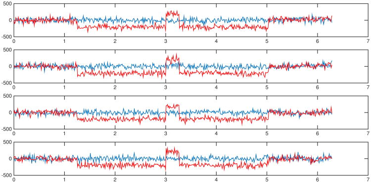
We simulate four pairs of signals y1(t) and y2(t), 0 ≤ t ≤ 2π:
| (28) |
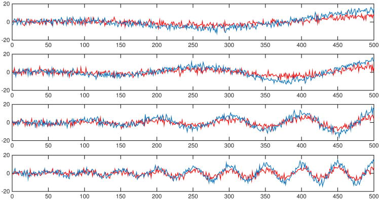
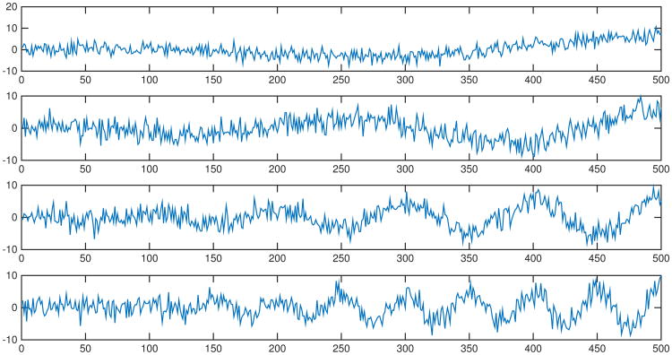
where ω takes on one of four values: 1) ω = 1; 2) ω = 2; 3) ω = 5; 4) ω = 10. Independent Gaussian noise N(0, 502) are added to the signals in each simulation (Figure 9). Percentages of p-values below 0.05 by different tests are summarized in Table 4. The results show that all three tests are fairly sensitive to the topologically invariant transformation at a threshold of 95%.
Fig 9.
Examples of the 4 signals given by (28) with noise. Blue curves are red curves undergone tearing transformations. Tests are performed on each pair of curves with independent Gaussian noises in each simulation.
Table 4.
Study 2 - percentages of p-values < 0.05 in 100 datasets simulated from the cosine functions (28) by baseline methods and the topological permutation test.
| Percentages of p-value < 0.05 | ω = 1 | ω = 2 | ω = 5 | ω = 10 |
|---|---|---|---|---|
|
| ||||
| Paired t-test on local variance | 93% | 93% | 93% | 95% |
| Paired t-test on PSD estimates | 100% | 100% | 100% | 100% |
| Topological permutation test | 90% | 93% | 93% | 95% |
5. Application to seizure EEGs
We apply the proposed topological permutation test to a single-trial multichannel epileptic EEG dataset to understand better the topological difference between signals before and during a seizure attack. The idea is to to explore topological information in univariate seizure signals via connected components in the sublevel set of each denoised signal. We compare results from the proposed method to baseline statistical features in the signal.
5.1. Description of the EEG Data
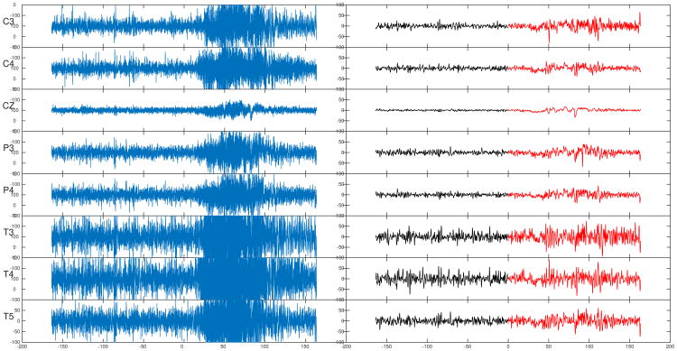
The single-trial multichannel EEG dataset were recorded from a patient of Dr. Malow (neurologist at the University of Michigan) (Ombao et al., 2001). Figure 10 shows a montage of the eight channels at which the EEG signals were sampled at a rate of 100 Hz for 32,680 time points. The female subject was already diagnosed with epilepsy on the left temporal lobe (approximately on the cortical surface directly below the T3 channel). In fact, this patient was determined to have a lesion located on the left temporal lobe and abnormal electrical activity in the brain is likely to be initiated from this region. Though it is well known that EEGs have relatively lower spatial resolution when compared to other imaging modalities (in order of centiimeter for EEG vs. millimeter for magnetic resonance imaging (MRI)), it is believed that electrical activity that is recorded at T3 and T5 is highly likely due to cortical activity on the cortical surface of the left temporal lobe. Thus there is an interest to focus our data analysis around the left temporal channels (T3 and T5). For this particular episode, the seizure initiates at the left temporal site (T3 channel) approximately halfway through the recording. Visual inspection of Figure 11 (left) shows the signals before seizure to be more stable (more stationary, lower variation, smaller magnitude of the waveforms) than the latter half. Highly volatile oscillations in the seizure period also seem to be concentrated in channels located near the T3 channel.
Fig 10.
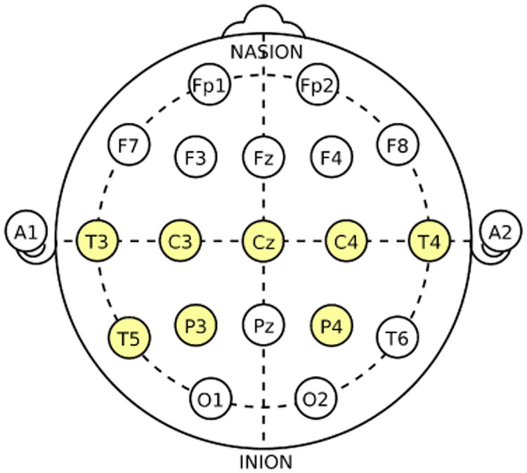
EEG channels in accordance with the international 10-20 system; T=temporal, P=parietal, C=central; odd (even) numbers indicate the left (right) hemisphere. Image source: https://en.wikipedia.org/wiki/10-20_system_(EEG).
Fig 11.
Left: EEG recording with a sampling rate of 100Hz over 163.4s; time 0 indicates the start of the seizure attack. Right: thresholded WFS denoising with degree k = 499 and bandwidth σ = 0.0001.
5.2. Results from the proposed method
As detailed in Section 3, each signal in the dataset undergoes denoising by a thresholded WFS (Figure 11 (right). Sine or cosine waveform are included in the representation if the corresponding amplitudes exceed some threshold. PLs are then constructed on each of the denoised signals. Figure 12 shows the PLs of denoised signals before and during seizure at all channels. These plots suggest that, up to scaling, the landscapes for the temporal channels (T3, T4, T5) appear to be very similar for both before and during seizure. For the remainder of the channels, the lanscapes are different.
Fig 12.
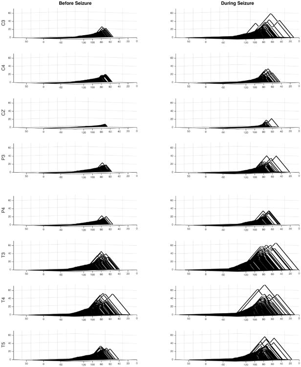
Persistence landscapes at all channels before and during seizure for signals denoised with WFS of degree k = 499 and bandwidth σ = 0.0001.
In the topological permutation test, the p-values are computed by counting the proportion of frequency-resampled PLs having L2 distances exceeding that of the observed PLs before and during seizure. The results obtained through 10,000 resamples with respect to multiple combinations of WFS degrees and bandwidths are summarized in Table 5. Our approach here was to be very conservative and thus we imposed a Bonferroni corrected 5% significance level for the 8 simultaneous topological permutation tests.
Table 5.
Summary of p-values computed with the proposed topological method with respect to different combination of thresholded WFS degrees and bandwidths. The p-values above the Bonferroni threshold of 0.05/8=0.0063 are shaded in gray. We observe that T3, T4 and T5 consistently showing up as topological invariant before and during seizure according to the Bonferroni threshold.
| k = 99 | k = 499 | k = 999 | ||
|---|---|---|---|---|
| σ = 0.0005 | C3 | 0.0001 | 0.0001 | 0.0001 |
| C4 | 0.0009 | 0.0014 | 0.0026 | |
| Cz | 0.0001 | 0.0001 | 0.0001 | |
| P3 | 0.0072 | 0.0020 | 0.0022 | |
| P4 | 0.0003 | 0.0001 | 0.0003 | |
| T3 | 0.1975 | 0.0960 | 0.0934 | |
| T4 | 0.0255 | 0.0228 | 0.0464 | |
| T5 | 0.0435 | 0.1522 | 0.1723 | |
|
| ||||
| σ = 0.0001 | C3 | 0.0057 | 0.0010 | 0.0006 |
| C4 | 0.0054 | 0.0639 | 0.0445 | |
| Cz | 0.0001 | 0.0001 | 0.0001 | |
| P3 | 0.0029 | 0.0001 | 0.0001 | |
| P4 | 0.0001 | 0.3238 | 0.2848 | |
| T3 | 0.0661 | 0.0406 | 0.0682 | |
| T4 | 0.0162 | 0.1286 | 0.1397 | |
| T5 | 0.1044 | 0.3065 | 0.2608 | |
We observe that T3, T4 and T5 consistently showing up as topologically invariant (i.e., the topology before seizure is highly similar to that during seizure) after the Bonferroni correction. In particular, T3 and T5 have the least significant topological difference compared with T4. The observation coincides with the diagnosis of the left temporal lobe being the epileptogenic zone. It suggests that EEG signals in the epileptogenic zone even before a seizure attack already have similar topological patterns as those during the seizure. There is a strong likelihood that seizure originates from a “general area” around the left temporal and left central regions (as suggested by the method) but due to volume conduction in EEGs, one cannot precisely pinpoint the location of the seizure. The fact that T4, which is symmetric to T3 shows up as vaguely topological invariant may be down to the fact that the partial seizure originating around the left temporal region progresses to the other side of the brain. It is interesting that the proposed method was able to capture these features of the EEG signals which were overlooked by other methods that previously analyzed this same dataset.
5.3. Method comparison
We also need to check the performance of two baseline features against PH features on the same dataset, bearing in mind that we want the results to be informative of topological differentiation in EEG signals before and during a seizure attack.
Paired t-test on local variance
Local variance is a simplistic statistical approach that has given surprisingly accurate results in epileptogenic analysis (McSharry, Smith and Tarassenko, 2003; Mohseni, Maghsoudi and Shamsollahi, 2006). It is defined as
where x is a signal at one channel and 〈·〉 is the average taken over an window of a certain size. For inference, we split up the range in to before and during seizure phases, Then we performed paired t-test on the local variances in 10 windows in the two phases of each channel. Table 6 summarizes the results of p-values of the paired t-tests on local variances of raw signals. The results are not informative as all the p-values are too small to conclude that any particular channels are topologically invariant.
Table 6.
Summary of p-values of the paired t-tests on local variances of raw signals.
| Channel | p-values (in 10−45) |
|---|---|
|
| |
| C3 | 0.0001 |
| C4 | 0.0001 |
| Cz | 0.0001 |
| P3 | 0.0001 |
| P4 | 0.0001 |
| T3 | 0.6721 |
| T4 | 0.0001 |
| T5 | 0.0001 |
Paired t-test on spectrogram
We first performed the discrete short-time Fourier transform (DSTFT) to obtain the windowed Fourier coefficients
before and during seizure:
| (29) |
| (30) |
where j = 1, …, k (k is the degree of the discrete Fourier transform for a windowed segment), ℓ is the number of time points by which the initial time points of consecutive segments differ and L is the pre-specified window size. The window functions are meant to smooth out discontinuities at boundaries. The most popular windows in practice are Hamming, Hanning, Kaiser and Gaussian (Oppenheim and Schafer, 1989). Here we used the Hamming window of pre-specified length L:
A signal is driven through the window in individual segments; each segment is multiplied pointwise to the window function. The power spectral density (PSD) estimates are given by
| (31) |
These estimates are the same as the classical local Fourier periodograms. Table 7 summarizes the results of p-values of the paired t-tests on PSD estimates of raw signals. The results are not informative as all the p-values are too small to conclude that any particular channels are topologically invariant.
Table 7.
Summary of p-values of the paired t-tests on PSD estimates of raw signals.
| Channel | p-values (in 10−18) |
|---|---|
|
| |
| C3 | 0.0001 |
| C4 | 0.1112 |
| Cz | 0.0001 |
| P3 | 0.0001 |
| P4 | 0.0001 |
| T3 | 0.0001 |
| T4 | 0.0001 |
| T5 | 0.0001 |
Results on denoised signals
The same methods were applied to signals denoised with WFS at degree 99 and bandwidth 0.001. Table 8 summarizes the results of p-values of the paired t-tests on local variances and PSD estimates of signals denoised with WFS. Although the overall conclusions remain the same, we can see that denoising raises the p-values dramatically.
Table 8.
Summary of p-values of the paired t-tests on local variances of signals denoised with WFS of degree 99 and bandwidth 0.001. These results suggest a difference in the topological structures of signals before and during seizure.
| Channel | Local variance (in 10−7) | PSD estimates (in 10−7) |
|---|---|---|
| C3 | 0.0001 | 0.0012 |
| C4 | 0.0001 | 0.2013 |
| Cz | 0.0001 | 0.0472 |
| P3 | 0.0001 | 0.0192 |
| P4 | 0.0001 | 0.0245 |
| T3 | 0.0001 | 0.0004 |
| T4 | 0.4691 | 0.2884 |
| T5 | 0.0001 | 0.2701 |
6. Discussion
This paper explores the topological information in seizure EEGs through the evolution of connected components in the signals. The novelty and contribution of the proposed procedure are unique in several aspects. Denoising univariate EEG signals by a thresholded WFS helps stabilize the subsequent analysis of connected components in the signals. The proposed TDA procedure is also the first to incorporate PL in the analysis of connected components of EEG signals. The method is developed to stay robust under basic topology-preserving transformations of signals. In simulation studies, the test consistently reflects the underlying topological difference and invariance of two signals compared with the instability of baseline statistical features.
The application on the real data has demonstrated the potential utility of our proposed procedure for insight on epileptogenicity. Previous analysis on the same data only showed the evolution of the spectral power and coherence during the seizure episode but did not identify seizure location (Ombao et al., 2001; Ombao, von Sachs and Guo, 2005). Neurologists can use this tool to guide them to examining further those regions that show topological invariance during the seizure episode.
The frequency resampling procedure serves the purpose of creating a sample of multiple trials from the single-trial dataset. Conclusions on the clinical population of epilepsy patients should be avoided (Maris, 2012). Additional analysis was performed on the middle 24000 and 30000 instead of the full 32680 time points of each of the 8 EEG signals denoised with WFS of degree k = 499 and bandwidths σ = 0.0005 and σ = 0.0001. The p-values above the Bonferroni threshold 0.05/8=0.0063 are again considered as topologically invariant. For the bandwidth σ = 0.0001, the patten of topological invariance remains the same for the two datasets of shorter lengths; for σ = 0.0005, the pattern varies while T5 remains topologically invariant. For further validation, the current method should be extended to large-scale multi-trial seizure EEG datasets, in which case multi-trial data would replace the subsamples created by the frequency resampling procedure.
Also, the proposed topological method is based on WFS of a fixed degree and bandwidth. The bandwidth σ modulates the smoothness of the WFS estimation. Given a certain σ, increasing the degree k increases the goodness of fit of the WFS series representation. However, having a large k can affect computational efficiency There is no unique way of optimal degree selection - for example one might use an F-test to compare two series expansions with different degrees (Chung et al., 2010). In the current study, we demonstrate the robustness of the procedure by testing out various combinations of small σ and large k for optimal representation. We also recommend practitioners to base their evaluation with respect to a reasonable range of σ and k. A data-driven automatic selection of these tuning parameters is beyond the scope of this paper. For future studies, an interesting direction worth pursuing is weighting persistence landscapes across different bandwidths of the WFS. We currently present results with respect to separate sets of parameters. Weighting the topological features across the parameters may improve efficiency in analysis.
Acknowledgments
The study is funded by NIH Brain Initiative grant R01 EB022856. We also like to thank anonymous reviewers for constructive criticisms that improved the paper.
Footnotes
MSC 2010 subject classifications: Primary 97K80; secondary 92B15
References
- Abramovich F, Benjamini Y. Adaptive thresholding of wavelet coefficients. Computational Statistics and Data Analysis. 1996;22:351–361. [Google Scholar]
- Ahmed M, Fasy BT, Wenk C. Local persistent homology based distance between maps. Proc ACM SIGSPATIAL GIS. 2014:43–52. [Google Scholar]
- Bancaud J, Brunet-Bourgin F, Chauvel P, Halgren E. Anatomical origin of déjà vu and vivid memories in human temporal lobe epilepsy. Brain. 1994;117:71–90. doi: 10.1093/brain/117.1.71. [DOI] [PubMed] [Google Scholar]
- Bartolomei F, Chauvel P, Wendling F. Epileptogenicity of brain structures in human temporal lobe epilepsy: A quantified study from intracerebral EEG. Brain. 2008;131:1818–1830. doi: 10.1093/brain/awn111. [DOI] [PubMed] [Google Scholar]
- Bendich P, Marron JS, Miller E, Pieloch A, Skwerer S. Persistent homology analysis of brain artery trees. Annals of Applied Statistics. 2016;10:198–218. doi: 10.1214/15-AOAS886. [DOI] [PMC free article] [PubMed] [Google Scholar]
- Botev ZI, Grotowski JF, Kroese DP. Kernel density estimation via diffusion. The Annals of Statistics. 2010;38:2916–2957. [Google Scholar]
- Bubenik P. Statistical topological data analysis using persistence landscapes. Journal of Machine Learning Research. 2015;16:77–102. [Google Scholar]
- Bubenik P, Carlson G, Kim PT, Luo ZM. Statistical topology via morse theory persistence and nonparametric estimation. Algebraic Methods in Statistics and Probability II Contemporary Mathematics. 2010;516:75–92. [Google Scholar]
- Carlsson G. Topology and data. Bulletin of the American Mathematical Society 2009 [Google Scholar]
- Chaudhuri P, Marron JS. Scale space view of curve estimation. The Annals of Statistics. 2000;28:408–428. [Google Scholar]
- Chazal F, Fasy BT, Lecci F, Michel B, Rinaldo A, Wasserman L. Subsampling methods for persistent homology. arXiv 1406.1901. 2014:1–16. [Google Scholar]
- Chung MK, Bubenik P, Kim PT. Information Processing in Medical Imaging. Springer; 2009. Persistence diagrams of cortical surface data; pp. 386–397. [DOI] [PubMed] [Google Scholar]
- Chung M, Dalton K, Shen L, Evans AC, Davidson RJ. Weighted Fourier series representation and its application to quantifying the amount of gray matter. Special Issue of IEEE Transactions on Medical Imaging on Computational Neuroanatomy. 2007;26:566–581. doi: 10.1109/TMI.2007.892519. [DOI] [PubMed] [Google Scholar]
- Chung MK, Adluru N, Lee JE, Lazar M, Lainhart JE, Alexander AL. Cosine series representation of 3D curves and its application to white matter fiber bundles in diffusion tensor imaging. Statistics and Its Interface. 2010;3:69–80. doi: 10.4310/sii.2010.v3.n1.a6. [DOI] [PMC free article] [PubMed] [Google Scholar]
- Chung MKM, Schaefer SSM, van Reekum CMM, Peschke-Schmitz L, Sutterer MJM, Davidson RJJ. A unified kernel regression for diffusion wavelets on manifolds detects aging-related changes in the amygdala and hippocampus. 17th International Conference on Medical Image Computing and Computer Assisted Intervention (MICCAI) 2014 doi: 10.1007/978-3-319-10470-6_98. [DOI] [PMC free article] [PubMed] [Google Scholar]
- Cohen-Steiner D, Edelsbrunner H, Harer J. Stability of persistence diagrams. Discrete and Computational Geometry. 2007;37:103–120. [Google Scholar]
- Cohen-Steiner D, Edelsbrunner H. Lipschitz functions have Lp-stable persistence. Foundations of Computational Mathematics. 2009;10:127–139. [Google Scholar]
- Donoho DL, Johnstone JM. Ideal spatial adaptation by wavelet shrinkage. Biometrika. 1994;81:425–455. [Google Scholar]
- Donoho DL, Johnstone IM. Adapting to unknown smoothness via wavelet shrinkage. Journal of the American Statistical Association. 1995;90:1200–1224. [Google Scholar]
- Donoho D, Mallat S, von Sachs R. Estimating covariances of locally stationary processes: rates of convergence of best basis methods Technical Report. Department of Statistics, Stanford University; Stanford: 1998. [Google Scholar]
- Edelsbrunner H, Harer J. Computational Topology. American Mathematical Society; 2010. [Google Scholar]
- Edelsbrunner H, Letscher D, Zomorodian A. Topological persistence and simplification. Discrete & Computational Geometry. 2002;28:511–533. [Google Scholar]
- Fried I. Auras and experiential responses arising in the temporal lobe. The Journal of Neuropsychiatry and Clinical Neurosciences. 1997;9:420–8. doi: 10.1176/jnp.9.3.420. [DOI] [PubMed] [Google Scholar]
- Gamble J, Heo G. Exploring uses of persistent homology for statistical analysis of landmark-based shape data. Journal of Multivariate Analysis. 2010;101:2184–2199. [Google Scholar]
- Heo G, Gamble J, Kim PT. Topological analysis of variance and the maxillary complex. Journal of the American Statistical Association. 2012;107:477–492. [Google Scholar]
- Khalid A, Kim BS, Chung MK, Ye JC, Jeon D. Tracing the evolution of multi-scale functional networks in a mouse model of depression using persistent brain network homology. NeuroImage. 2014;101:351–63. doi: 10.1016/j.neuroimage.2014.07.040. [DOI] [PubMed] [Google Scholar]
- Kobau R, Luo Y, Zack M, Helmers S, Thurman D. Epilepsy in adults and access to care - United States, 2010. Morbidity and Mortality Weekly Report. 2012;61:910–913. [PubMed] [Google Scholar]
- Lee H, Chung MK, Kang H, Kim BN, Lee DS. Computing the shape of brain networks using graph filtration and Gromov-Hausdorff metric. MICCAI International Conference on Medical Image Computing and Computer-Assisted Intervention. 2011;14:302–9. doi: 10.1007/978-3-642-23629-7_37. [DOI] [PubMed] [Google Scholar]
- Maris E. Statistical testing in electrophysiological studies. Psychophysiology. 2012;49:549–565. doi: 10.1111/j.1469-8986.2011.01320.x. [DOI] [PubMed] [Google Scholar]
- Martinerie J, Adam C, Le Van Quyen M, Baulac M, Clémenceau S, Renault B, Varela F. Can epileptic seizure be anticipated by nonlinear analysis? Nature Medicine. 1998;4:1173–1176. doi: 10.1038/2667. [DOI] [PubMed] [Google Scholar]
- McSharry PE, Smith La, Tarassenko L. Prediction of epileptic seizures: are nonlinear methods relevant? Nature Medicine. 2003;9:241–242. doi: 10.1038/nm0303-241. author reply 242. [DOI] [PubMed] [Google Scholar]
- Mileyko Y, Mukherjee S, Harer J. Probability measures on the space of persistence diagrams. Inverse Problems. 2011;27:1–21. [Google Scholar]
- Mitra PP, Pesaran B. Analysis of dynamic brain imaging data. Biophysical Journal. 1999;76:691–708. doi: 10.1016/S0006-3495(99)77236-X. [DOI] [PMC free article] [PubMed] [Google Scholar]
- Mohseni HRHR, Maghsoudi A, Shamsollahi MBMB. Seizure detection in EEG signals: a comparison of different approaches; Annual International Conference of the IEEE Engineering in Medicine and Biology Society IEEE Engineering in Medicine and Biology Society; 2006. pp. 6724–6727. [DOI] [PubMed] [Google Scholar]
- Munkres JR. Elements of Algebraic Topology. Addison-Wesley; 1984. [Google Scholar]
- Ombao H, von Sachs R, Guo W. SLEX analysis of multivariate nonstationary time series. Journal of the American Statistical Association. 2005;100:519–531. [Google Scholar]
- Ombao HC, Raz JA, von Sachs R, Malow BA. Automatic statistical analysis of bivariate nonstationary time series. Journal of the American Statistical Association. 2001;96:543–560. [Google Scholar]
- Oppenheim AV, Schafer RW. Discrete-Time Signal Processing. Third. Prentice-Hall Signal Processing Series; 1989. [Google Scholar]
- Petri G, Scolamiero M, Donato I, Vaccarino F. Topological strata of weighted complex networks. PLoS ONE. 2013;8 doi: 10.1371/journal.pone.0066506. [DOI] [PMC free article] [PubMed] [Google Scholar]
- Politis DN, Romano JP, Wolf M. Subsampling. Springer; New York: 1999. [Google Scholar]
- Sousbie T, Pichon C, Kawahara H. The persistent cosmic web and its filamentary structure. Monthly Notices of the Royal Astronomical Society. 2011;414:384–403. [Google Scholar]
- Turner K, Mileyko Y, Mukherjee S, Harer J. Frechet means for distributions of persistence diagrams. Discrete & Computational Geometry. 2014;52:44–70. [Google Scholar]
- WHO. Atlas: epilepsy care in the world Technical Report 2005 [Google Scholar]


