Mathematical Analysis of Influenza A Dynamics in the Emergence of Drug Resistance

Abstract

Every year, influenza causes high morbidity and mortality especially among the immunocompromised persons worldwide. The emergence of drug resistance has been a major challenge in curbing the spread of influenza. In this paper, a mathematical model is formulated and used to analyze the transmission dynamics of influenza A virus having incorporated the aspect of drug resistance. The qualitative analysis of the model is given in terms of the control reproduction number, R_c. The model equilibria are computed and stability analysis carried out. The model is found to exhibit backward bifurcation prompting the need to lower R_c to a critical value R_c^∗ for effective disease control. Sensitivity analysis results reveal that vaccine efficacy is the parameter with the most control over the spread of influenza. Numerical simulations reveal that despite vaccination reducing the reproduction number below unity, influenza still persists in the population. Hence, it is essential, in addition to vaccination, to apply other strategies to curb the spread of influenza.

1. Introduction

Influenza is a contagious respiratory illness caused by influenza viruses. There are three major types of flu viruses: types A, B, and C. The majority of human infections are caused by types A and B. Of major concern is influenza A virus which is clinically the most vicious. It is a negative-sense single-stranded RNA virus with eight gene segments. The segmented nature of influenza A virus genome allows the exchange of gene segments between viruses that coinfect the same cell [1]. This process of genetic exchange is termed reassortment. Reassortment leads to sudden changes in viral genetics and to susceptibility in hosts. Influenza A virus has a wide range of susceptible avian hosts and mammalian hosts such as humans, pigs, horses, seals, and mink. In addition, the virus is able to repeatedly switch hosts to infect multiple avian and mammalian species. The unpredictability of influenza A virus evolution and interspecies movement creates continual public health challenges [2].

Influenza A virus constantly mutates and is able to elude the immune system of an individual. It can mutate in two different ways: antigenic shift and antigenic drift. Antigenic shift is an abrupt, major change in the influenza virus which happens occasionally and results in a new subtype that most people have no protection against. Such a shift occurred in the spring of 2009 in Mexico and United States, when H1N1 virus with a new combination of genes emerged to infect people and quickly spread, causing a pandemic [3]. This antigenic shift was as a result of extensive reassortment in swine that brought together genes from avian, swine, and human flu viruses [4]. On the other hand, antigenic drift refers to small changes in the genes of influenza viruses that occur continually as the virus replicates. Over time, these small genetic changes result in new strains which the antibodies can no longer recognize. The changes in the influenza viruses are the main reason why individuals are infected with the flu more than once. The viruses infect the nose, throat, and lungs. They usually are spread through the air when the infected people cough, sneeze, or talk making the surrounding air and surfaces to be temporarily contaminated with infected droplets [5, 6]. People get infected when they inhale the infected droplets. A person might also get flu by touching the surface or object that has flu virus on it and then touching their own mouth, eyes, or possibly their nose [6].

Influenza can be prevented by getting vaccination each year. However, given that the virus mutates rapidly, a vaccine made for one year may not be useful in the following year. In addition, antigenic drift in the virus may occur after the year's vaccine has been formulated, rendering the vaccine less protective, and hence, outbreaks can easily occur especially among high-risk individuals [7]. According to [8], other preventive actions include staying away from people who are sick, covering coughs and sneezes, and frequent handwashing.

Influenza spreads rapidly around the world during seasonal epidemics and pandemics [9]. It has afflicted the human population for centuries. For instance, the 1918 influenza pandemic infected nearly one quarter of the world's population and resulted in the deaths of about 100 million people [10]. Studies show that this pandemic is especially responsible for the high morbidity and mortality among vulnerable groups such as children, the elderly, and patients with underlying health conditions [11]. Within the past one hundred years, there have been four pandemics resulting from the emergence of a novel influenza strain for which the human population possessed little or no immunity. Table 1 gives a brief summary of the four influenza pandemics.

Table 1.

Summary of influenza pandemics in the past one hundred years.

Pandemic name	Year	Strain	Approximate number of deaths
Spanish flu	1918–1920	H1N1	40–100 million
Asian flu	1957–1958	H2N2	1–2 million
Hong Kong flu	1968–1970	H3N2	0.5–2 million
Swine flu	2009–2010	H1N1	Up to 575,000

Source: [10, 12, 13].

Besides the influenza pandemics, there is an outbreak of influenza every year around the world which results in about three to five million cases of severe illness and about 250,000 to 500,000 deaths [14]. According to a report by Centers for Disease Control and Prevention (CDC), as of December 2017, the estimated number of deaths worldwide resulting from seasonal influenza had risen to between 291,000 and 646,000 [15]. This new estimate was from a collaborative study by CDC and global health partners. In the temperate northern hemisphere (i.e., north of the Tropic of Cancer) and temperate southern hemisphere (i.e., south of the Tropic of Capricorn), influenza has been observed to peak in the winter months [16, 17]. In tropical regions, influenza seasonality is less obvious and epidemics can occur throughout the year and more specifically during the rainy seasons [18]. According to [19], the mortality rates due to this respiratory disease are much higher in Africa than anywhere else in the world. Poor nutritional status, poor access to healthcare including vaccination and antibiotics, and the presence of other, less measurable factors related to poverty in Africa may be additional risk factors for higher mortality rates. WHO Global Influenza Surveillance and Response System (GISRS) monitors the evolution of influenza viruses. Figures 1 and 2 show the global circulation of influenza viruses from 2016 to week 24 of 2018 [20, 21].

Figure 1.

Global circulation of influenza viruses from 2016 to 2017.

Figure 2.

Global circulation of influenza viruses from 2017 to week 24 of 2018.

Influenza-attributable mortality varies across the seasons. There is however paucity of published estimates of influenza mortality for low- and middle-income countries. Data from Centers for Disease Control and Prevention (CDC) databases from the 1999–2000 to the 2014–2015 seasons for the U.S. population aged 65 years and above were used to estimate excess deaths per month over that 15-year span [22]. The data are presented in Figure 3.

Figure 3.

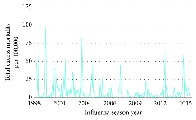
Excess mortality due to influenza for the U.S. population aged 65 years and above.

In addition to pandemics and seasonal epidemics caused by influenza A virus, over the past 20 years, multiple zoonotic influenza A virus outbreaks have occurred causing a great concern to public health [23–26]. For instance, H5N1 influenza virus from avian hosts poses an ongoing threat to human and animal health due to its high mortality rate [26–28]. H7N9 is yet another highly pathogenic subtype of influenza A virus that is of major concern. According to the World Health Organization (WHO), as of January 2018, 1566 laboratory-confirmed cases of human infection with H7N9 virus have been reported in China, including at least 613 deaths [29]. In addition to the ongoing H5N1 and H7N9 influenza A virus outbreaks, other subtypes, such as H5N6, H9N2, H10N8, and H6N1, have sporadically caused serious human infections in China and Taiwan [30–33]. The death toll from influenza is unacceptably high, given that it is preventable. Efforts to combat it must therefore be accelerated. In view of the catastrophic effects of influenza globally, several models have been proposed and analyzed with the aim of shedding more light in the transmission dynamics of influenza, for instance [34–41]. Among the pioneer mathematical models used to describe influenza dynamics is one developed by [38].

Emergence of drug resistance which is a growing menace globally [42] complicates influenza even more [43, 44]. Drug resistance refers to reduction in the effectiveness of a drug in curing a disease. It occurs when microorganisms such as bacteria, viruses, fungi, and parasites change in ways that render the medications used to cure the infections they cause ineffective [45, 46]. The microorganisms are therefore able to survive the treatment. According to [47], epidemics with drug-resistant strains and those with drug-sensitive strains are fundamentally different in their growth and dynamics. Drug-sensitive epidemics are fuelled by only one process, that is, transmission; however, drug-resistant epidemics are fuelled by two processes: transmission and the conversion of treated drug-sensitive infections to drug-resistant infections (acquired resistance). Therefore, the rate of increase in drug-resistant infections can be much faster than the rate of increase in drug-sensitive infections. Studies from [48] show that drug resistance is a function of time and treatment rate. In addition, immunosuppression especially in individuals with compromised immune systems contributes to lack of viral clearance often despite antiviral therapy leading to emergence of antiviral resistance [49].

There are two classes of antiviral drugs that are used to treat influenza: adamantanes and neuraminidase inhibitors. The adamantanes are only effective against influenza A viruses, as they inhibit the M2 protein, which is not coded by influenza B [50]. These drugs are associated with several toxic effects and rapid emergence of drug-resistant strains. The neuraminidase inhibitors interfere with the release of progeny influenza virus from infected host cells, a process that prevents infection of new host cells and thereby halts the spread of infection in the respiratory tract [7]. Since these drugs act at the stage of viral replication, they must be administered as early as possible. According to [51], influenza viruses mutate constantly, either from one season to the next or within the course of one flu season. As a flu virus replicates, the genetic makeup may change rendering the virus resistant to one or more of the antiviral drugs used to treat or prevent influenza. Antiviral resistance in influenza may not only emerge during treatment but also sometimes transmit widely to replace wild-type strains in the absence of drug pressure. The transmission of resistant strains is evidenced by the global spread of adamantane-resistant A(H3N2) viruses since 2003, oseltamivir-resistant seasonal A(H1N1) viruses since 2007, and adamantane-resistant pandemic A(H1N1) viruses in 2009, leading to increased challenges in the management of influenza [52]. With the development of drug-resistant influenza viruses, various models have also been formulated in order to understand this phenomenon better. Among them are [53–57].

The morbidity, mortality, and economic burden of influenza cannot be overlooked. With the emerging menace of drug resistance, this burden becomes even more complicated. In order to curb the spread of influenza, there is a dire need to understand among its many aspects, its transmission dynamics especially in light of the drug resistance aspect. In this paper, a mathematical model that illustrates the transmission dynamics of a wild-type influenza strain and the development and transmission of drug-resistant influenza strain is formulated and analyzed.

2. Mathematical Model

2.1. Model Formulation

The model subdivides the total population into five compartments: Susceptible (S), Vaccinated (V), Infected with Wild-type strain (I_w), Infected with Resistant strain (I_R), and Recovered (R). Individuals in a given compartment are assumed to have similar characteristics. Parameters vary from compartment to compartment but are identical for all individuals in a given compartment. Individuals enter the population at the rate of π, and all recruited individuals are assumed to be susceptible. The Susceptible get infected after effective contact with either the Infected with Wild-type strain or the Infected with Resistant strain. The force of infection is given by either λ₁=β_wI_w (Infection by Wild-type strain) or ${\lambda }_2=\overline{{\beta }_{\text{r}}}{I}_{\text{R}}$ (Infection by Resistant strain), where $\overline{{\beta }_{\text{r}}}=f\left({\beta }_{\text{r}},\hspace{0.17em}\hspace{0.17em}b\right)$. Parameters β_w and β_r refer to the transmission rate of wild-type strain and resistant strain, respectively. Parameter b is the rate of developing drug resistance. The susceptible can only be infected by one strain at a time. The rate of vaccination is ϕ. The vaccinated can also become infected with either the wild-type strain or the resistant strain. This depends on the vaccine efficacy. When the vaccine efficacy is 100%, the vaccinated cannot become infected. Individuals who are infected with the wild-type strain are treated and recover at the rate of α, while those who are infected with the resistant strain recover at the rate of α_r. The wild-type strain is assumed to mutate to resistant strain, and hence, those infected with the wild type join those infected with the resistant strain at the rate of b. Individuals with wild-type strain and those with resistant strain suffer disease-induced death at the rates a_w and a_r, respectively. The recovered lose immunity at the rate of ϑ joins the susceptible class. Individuals in all the epidemiological compartments suffer natural death at the rate of μ. The model diagram is given in Figure 4.

Figure 4.

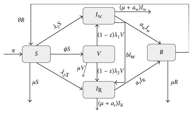
Schematic diagram showing population flow between different epidemiological classes.

2.2. Model Equations

Given the dynamics described in Figure 4, the following system of nonlinear ordinary differential equations, with nonnegative initial conditions, describes the dynamics of influenza:

$$\begin{array}{c}\frac{dS}{dt}=\pi +\vartheta R-\left(\varphi +\mu +{\lambda }_1+{\lambda }_2\right)S\left(t\right),\\ \frac{dV}{dt}=\varphi S\left(t\right)-\left(\left(1-\epsilon \right){\lambda }_1+\left(1-\epsilon \right){\lambda }_2+\mu \right)V\left(t\right),\\ \frac{d{I}_w}{dt}={\lambda }_{1}S\left(t\right)+\left(1-\epsilon \right){\lambda }_{1}V\left(t\right)-\left(b+\mu +a_w+\alpha \right)I_w\left(t\right),\\ \frac{d{I}_{\text{R}}}{dt}={\lambda }_{2}S\left(t\right)+\left(1-\epsilon \right){\lambda }_{2}V\left(t\right)+b{I}_w\left(t\right)-\left(\mu +{\alpha }_{\text{r}}+a_{\text{r}}\right)I_{\text{R}}\left(t\right),\\ \frac{dR}{dt}=\alpha I_w\left(t\right)+{\alpha }_{\text{r}}{I}_{\text{R}}\left(t\right)-\left(\vartheta +\mu \right)R\left(t\right),\end{array}$$ (1)

where λ₁=β_wI_w and λ₂=β_r(1+b²)I_R.

We assume that all the model parameters are positive and the initial conditions of the model system (1) are given by

$$\begin{array}{c}S\left(0\right)>0,\hspace{0.17em}\hspace{0.17em}V\left(0\right)\ge 0,\hspace{0.17em}\hspace{0.17em}{I}_{\text{W}}\left(0\right)\ge 0,\hspace{0.17em}\hspace{0.17em}{I}_R\left(0\right)\ge 0,\hspace{0.17em}\hspace{0.17em}R\left(0\right)\ge 0.\end{array}$$ (2)

Table 2 gives the description of the various parameters used in the model along with reasonable estimates of their values.

Table 2.

Description and values of parameters used.

Parameter	Description	Value	Reference
β w	Transmission rate of wild-type strain	0.00102 day−1	Estimated
β r	Transmission rate of resistant strain	0.00026 day−1	Estimated
ε	Vaccine efficacy	0.77	[58]
ϕ	Vaccination rate	0.00027375 day−1	[59]
b	Rate of developing drug resistance	0.118	Estimated
α	Recovery rate for individuals in Iw class	0.1998 day−1	[6]
α r	Recovery rate for individuals in IR class	0.0714 day−1	Estimated
ϑ	Rate of losing immunity	0.00833 day−1	[34]
a w	Death rate due to infection with wild-type strain	0.01	[39]
$\frac{1}{\mu }$	Average human lifespan	70 × 365 days	Estimated
π	Recruitment rate	0.0381	Estimated
a r	Death rate due to infection with resistant strain	0.021	Estimated

3. Model Analysis

3.1. Basic Properties

3.1.1. Positivity of Solutions

The model system (1) monitors the changes in human population. It is therefore important to prove that the solutions of system (1) with nonnegative initial conditions will remain nonnegative for all t > 0. Thus, we have the following theorem:

Theorem 1 . —

Given that the initial conditions of system (1) areS(0) > 0, V(0) ≥ 0, I_W(0) ≥ 0, I_R(0) ≥ 0, and  R(0) ≥ 0, the solutionsS(t), V(t), I_w(t), I_R(t), and  R(t)are nonnegative for allt > 0.

Proof —

Assume that

$$\begin{array}{c}\widehat{t}=\sup \left\{t>0\hspace{0.17em}\hspace{0.17em}:\hspace{0.17em}\hspace{0.17em}S\left(t\right)>0,\hspace{0.17em}\hspace{0.17em}V\left(t\right)>0,\hspace{0.17em}\hspace{0.17em}{I}_w\left(t\right)>0,\hspace{0.17em}\hspace{0.17em}{I}_{\text{R}}\left(t\right)>0,\hspace{0.17em}\hspace{0.17em}R\left(t\right)>0\right\}\in \left[0,\hspace{0.17em}\hspace{0.17em}t\right].\end{array}$$ (3)

Thus $\widehat{t}>0$, and it follows directly from the first equation of system (1) that

$$\begin{array}{c}\frac{dS}{dt}\ge \pi -\left({\lambda }_1+{\lambda }_2+\mu \right)S.\end{array}$$ (4)

Using the integrating factor method to solve inequality (4), we have

$$\begin{array}{c}\frac{d}{dt}\left\{S\left(t\right)\hspace{0.17em}\hspace{0.17em}\exp \left[\mu t+{{{\displaystyle \int }}^{}}_0^t\left({\lambda }_1\left(s\right)+{\lambda }_2\left(s\right)\right)ds\right]\right\}\ge \pi \hspace{0.17em}\hspace{0.17em}\exp \left[\mu t+{{{\displaystyle \int }}^{}}_0^t\left({\lambda }_1\left(s\right)+{\lambda }_2\left(s\right)\right)ds\right].\end{array}$$ (5)

Integrating both sides yields

$$\begin{array}{c}S\left(\widehat{t}\right)\hspace{0.17em}\hspace{0.17em}\exp \left[\mu \widehat{t}+{{{\displaystyle \int }}^{}}_0^{\widehat{t}}\left({\lambda }_1\left(s\right)+{\lambda }_2\left(s\right)\right)ds\right]\ge {{{\displaystyle \int }}^{}}_0^{\widehat{t}}\pi \hspace{0.17em}\hspace{0.17em}\exp \left[\mu \widehat{t}+{{{\displaystyle \int }}^{}}_0^{\widehat{t}}\left({\lambda }_1\left(w\right)+{\lambda }_2\left(w\right)\right)dw\right]d\widehat{t}+C,\end{array}$$ (6)

where C is the constant of integration. Hence,

$$\begin{array}{c}S\left(\widehat{t}\right)\ge S\left(0\right)\hspace{0.17em}\hspace{0.17em}\exp \left[-\left(\mu \widehat{t}+{{{\displaystyle \int }}^{}}_0^{\widehat{t}}\left({\lambda }_1\left(s\right)+{\lambda }_2\left(s\right)\right)ds\right)\right]+\exp \left[-\left(\mu \widehat{t}+{{{\displaystyle \int }}^{}}_0^{\widehat{t}}\left({\lambda }_1\left(s\right)+{\lambda }_2\left(s\right)\right)ds\right)\right]\left({{{\displaystyle \int }}^{}}_0^{\widehat{t}}\pi \hspace{0.17em}\hspace{0.17em}\exp \left[\mu \widehat{t}+{{{\displaystyle \int }}^{}}_0^{\widehat{t}}\left({\lambda }_1\left(w\right)+{\lambda }_2\left(w\right)\right)dw\right]d\widehat{t}\right)>0.\end{array}$$ (7)

Hence, $S\left(\widehat{t}\right)>0$∀$\widehat{t}>0$.

From the second equation in system (1), we obtain

$$\begin{array}{c}\frac{dV}{dt}\ge -\left(\left(1-\epsilon \right){\lambda }_1+\left(1-\epsilon \right){\lambda }_2+\mu \right)V.\end{array}$$ (8)

Hence,

$$\begin{array}{c}V\left(\widehat{t}\right)\ge V\left(0\right)\hspace{0.17em}\hspace{0.17em}\exp \left[-\left\{\mu \widehat{t}+{{{\displaystyle \int }}^{}}_0^{\widehat{t}}\left(1-\epsilon \right){\lambda }_1\left(s\right)+\left(1-\epsilon \right){\lambda }_2\left(s\right)ds\right\}\right]>0.\end{array}$$ (9)

Similarly, it can be shown that

$$\begin{array}{c}{I}_w\left(\widehat{t}\right)\ge I_w\left(0\right)\hspace{0.17em}\hspace{0.17em}\exp \left\{-\left(b+\alpha +a_w+\mu \right)\widehat{t}\right\}>0,\\ I_{\text{R}}\left(\widehat{t}\right)\ge I_{\text{R}}\left(0\right)\exp \left\{-\left({\alpha }_{\text{r}}+a_{\text{r}}+\mu \right)\widehat{t}\right\}>0,\\ R\left(\widehat{t}\right)\ge R\left(0\right)\hspace{0.17em}\hspace{0.17em}\exp \left\{-\left(\vartheta +\mu \right)\widehat{t}\right\}>0.\end{array}$$ (10)

Therefore, all the solutions of system (1) with nonnegative initial conditions will remain nonnegative for all time t > 0.

3.1.2. Invariant Region

We show that the total population is bounded for all time t > 0. The analysis of system (1) will therefore be analyzed in a region Ω of biological interest. Thus, we have the following theorem on the region that system (1) is restricted to.

Theorem 2 . —

The feasible regionΩdefined by

$$\begin{array}{c}\Omega =\left\{\left(S\left(t\right),\hspace{0.17em}\hspace{0.17em}V\left(t\right),\hspace{0.17em}\hspace{0.17em}{I}_{\text{W}}\left(t\right),\hspace{0.17em}\hspace{0.17em}{I}_{\text{R}}\left(t\right),\hspace{0.17em}\hspace{0.17em}R\left(t\right)\right)\in R_5^{+}\hspace{0.17em}\mid \hspace{0.17em}0\le N\le \max \left\{N\left(0\right),\frac{\Pi }{\mu }\right\}\right\},\end{array}$$ (11)

with initial conditionsS(0) ≥ 0, V(0) ≥ 0, I_W(0) ≥ 0, I_R(0) ≥ 0, and  R(0) ≥ 0, is positively invariant and attracting with respect to system (1) for allt > 0.

Proof —

Summing up the equations in (1), we obtain that the total population satisfies the following differential equation:

$$\begin{array}{c}\frac{dN\left(t\right)}{dt}=\pi -\mu N-a_w{I}_w-a_{\text{r}}{I}_{\text{R}}.\end{array}$$ (12)

In the absence of influenza infection, it follows that

$$\begin{array}{c}\frac{dN\left(t\right)}{dt}\le \pi -\mu N.\end{array}$$ (13)

It can easily be seen that

$$\begin{array}{c}N\left(t\right)\le \frac{\Pi }{\mu }+\left(N\left(0\right)-\frac{\Pi }{\mu }\right)\exp \left(-\mu t\right).\end{array}$$ (14)

From (14), we observe that as t → ∞, N(t) → (Π/μ). So if N(0) ≤ (Π/μ), then lim_t→∞N(t)=(Π/μ). On the other hand, if N(0) > (Π/μ), then N will decrease to (Π/μ) as t → ∞. This means that N(t) ≤ max{N(0), (Π/μ)}. Therefore, N(t) is bounded above. Subsequently, S(t), V(t), I_w(t), I_R(t), and  R(t) are bounded above. Thus, in Ω, system (1) is well posed. Hence, it is sufficient to study the dynamics of the system in Ω.

3.2. Existence of Equilibrium Points

In the absence of influenza (I_w=I_R=0), system (1) has a disease-free equilibrium, which is given by

$$\begin{array}{c}{E}_0=\left(S^0,\hspace{0.17em}\hspace{0.17em}{V}^0,\hspace{0.17em}\hspace{0.17em}0,\hspace{0.17em}\hspace{0.17em}0,\hspace{0.17em}\hspace{0.17em}0\right)=\left(\frac{\Pi }{\varphi +\mu },\hspace{0.17em}\hspace{0.17em}\frac{\varphi \Pi }{\mu \left(\varphi +\mu \right)},\hspace{0.17em}\hspace{0.17em}0,\hspace{0.17em}\hspace{0.17em}0,\hspace{0.17em}\hspace{0.17em}0\right).\end{array}$$ (15)

3.2.1. The Control Reproduction Number

The control reproduction number, R_c, is a key threshold that determines the behaviour of the system in the presence of vaccination. In order to analyze the stability of system (1), we obtain the threshold condition for the establishment of the disease. Thus, we employ next-generation matrix operator method as explained in [60]. The matrices of new infections and transition terms evaluated at the disease-free equilibrium are given by

$$\begin{array}{c}\mathbf{F}=\left[\begin{array}{cc}\frac{\Pi {\beta }_w\left(\varphi \left(1-\epsilon \right)+\mu \right)}{\mu \left(\mu +\varphi \right)}& 0\\ 0& \frac{\Pi \overline{{\beta }_{\text{r}}}\left(\varphi \left(1-\epsilon \right)+\mu \right)}{\mu \left(\mu +\varphi \right)}\end{array}\right],\\ \mathbf{V}=\left[\begin{array}{cc}b+\alpha +\mu +a_w& 0\\ -b& \mu +a_{\text{r}}+{\alpha }_{\text{r}}\end{array}\right].\end{array}$$ (16)

The dominant eigenvalue corresponding to the spectral radius ρ(FV⁻¹) of the matrix FV⁻¹ is the control reproduction number, which is given by

$$\begin{array}{c}{R}_{\text{c}}=\max \left\{R_{cw},\hspace{0.17em}\hspace{0.17em}{R}_{\text{cr}}\right\},\end{array}$$ (17)

where

$$\begin{array}{c}{R}_{cw}=\frac{{\beta }_w\pi \left(\mu +\varphi \left(1-\epsilon \right)\right)}{\mu \left(\varphi +\mu \right)\left(\alpha +b+a_w+\mu \right)},\\ R_{\text{cr}}=\frac{\overline{{\beta }_{\text{r}}}\pi \left(\mu +\left(1-\epsilon \right)\varphi \right)}{\mu \left(\varphi +\mu \right)\left({\alpha }_{\text{r}}+a_{\text{r}}+\mu \right)}.\end{array}$$ (18)

R_cw is a measure of the average number of secondary wild-type influenza infections caused by a single infected individual introduced into the model population. On the other hand, R_cr gives the average number of secondary resistant influenza infections caused by one infected individual introduced into the model population.

From Theorem 2 in [60], we have the following results.

Proposition 1 . —

The disease-free equilibrium is locally asymptotically stable whenever R_c is less than unity and unstable otherwise.

Proof —

The Jacobian matrix evaluated at E₀ is obtained as

$$\begin{array}{c}J\left(E_0\right)=\left[\begin{array}{ccccc}-\varphi -\mu & 0& -{\beta }_w{S}^0& -\overline{{\beta }_{\text{r}}}{S}^0& \vartheta \\ \varphi & -\mu & -\left(1-\epsilon \right){\beta }_w{V}^0& -\left(1-\epsilon \right)\overline{{\beta }_{\text{r}}}{V}^0& 0\\ 0& 0& {\beta }_w{S}^0+\left(1-\epsilon \right){\beta }_w{V}^0-Q_1& 0& 0\\ 0& 0& b& \overline{{\beta }_{\text{r}}}{S}^0+\left(1-\epsilon \right)\overline{{\beta }_{\text{r}}}{V}^0-Q_2& 0\\ 0& 0& \alpha & {\alpha }_{\text{r}}& -\vartheta -\mu \end{array}\right],\end{array}$$ (19)

where Q₁=α+b+a_w+μ and Q₂=α_r+a_r+μ.

For the DFE to be locally stable, the eigenvalues of J(E₀) must have negative real parts.

The characteristic polynomial of J(E₀) is given by

$$\begin{array}{c}P\left(\lambda \right)=\left(\lambda +\mu \right)\left(\lambda +\mu +\vartheta \right)\left(\lambda +\mu +\varphi \right)\left(\mu \left(\mu +\varphi \right)\left(a_{\text{r}}+\lambda +\mu +{\alpha }_{\text{r}}\right)-\Pi \overline{{\beta }_{\text{r}}}\left(\mu -\epsilon \varphi +\varphi \right)\right)\left(\mu \left(\mu +\varphi \right)\left(a_w+\alpha +b+\lambda +\mu \right)-\Pi {\beta }_w\left(\mu -\epsilon \varphi +\varphi \right)\right).\end{array}$$ (20)

Clearly, the following eigenvalues with negative real parts can be obtained from the polynomial (20): λ₁=−μ, λ₂=−μ − ϑ, and  λ₃=−μ − ϕ. Other roots can be obtained from the remaining part of the polynomial (20), which is given by

$$\begin{array}{c}{P}_1\left(\lambda \right)=\left(\mu \left(\mu +\varphi \right)\left(a_{\text{r}}+\lambda +\mu +{\alpha }_{\text{r}}\right)-\Pi \overline{{\beta }_{\text{r}}}\left(\mu -\epsilon \varphi +\varphi \right)\right)\left(\mu \left(\mu +\varphi \right)\left(a_w+\alpha +b+\lambda +\mu \right)-\Pi {\beta }_w\left(\mu -\epsilon \varphi +\varphi \right)\right).\end{array}$$ (21)

Hence, we obtain

$$\begin{array}{c}{\lambda }_4=\frac{-\mu \left(\mu +\varphi \right)\left(a_{\text{r}}+\mu +{\alpha }_{\text{r}}\right)+\pi \overline{{\beta }_{\text{r}}}\left(\mu +\varphi \left(1-\epsilon \right)\right)}{\mu \left(\mu +\varphi \right)},\\ \therefore {\lambda }_4=-Q_2\left(1-R_{\text{cr}}\right),\\ {\lambda }_5=\frac{-\mu \left(\mu +\varphi \right)\left(b+\alpha +\mu +a_w\right)+\pi {\beta }_w\left(\mu +\varphi \left(1-\epsilon \right)\right)}{\mu \left(\mu +\varphi \right)},\\ \therefore {\lambda }_5=-Q_1\left(1-R_{cw}\right).\end{array}$$ (22)

From (22), if R_cr < 1, then λ₄ < 0, and if R_cw < 1, then λ₅ < 0.

We therefore conclude that the disease-free equilibrium E₀ is locally asymptotically stable whenever R_c < 1. The biological implication of Proposition 1 is that if R_c < 1, influenza will be eliminated from the model population provided that the initial sizes of the subpopulations in various compartments of model (1) are in the basin of attraction of the influenza-free equilibrium.

3.2.2. Effective Reproduction Number

The effective reproduction number (R_e(t)) is the actual average number of secondary cases per primary case at calendar time t (for t > 0) [61]. R_e(t) shows time-dependent variation due to decline in susceptible individuals and the implementation of control measures. The effective reproduction number is therefore used to characterize transmissibility in a population that is not entirely susceptible. It is the basic reproduction number times the fraction of the population that is susceptible to infection at time t.

The basic reproduction number (R₀) is the average number of secondary infections generated by a single infective individual in a totally susceptible population [60]. From model (1), the basic reproduction number is obtained as

$$\begin{array}{c}{R}_0=\max \left\{\frac{{\beta }_w\pi \mu }{{\mu }^2\left(\alpha +b+a_w+\mu \right)},\frac{\overline{{\beta }_{\text{r}}}\pi \mu }{{\mu }^2\left({\alpha }_{\text{r}}+a_{\text{r}}+\mu \right)}\right\}.\end{array}$$ (23)

Thus, the effective reproduction number R_e(t) = fR₀, where f is the fraction of population susceptible to infection at a time t.

3.3. Endemic Equilibria

The endemic equilibria of model (1)are the steady states where influenza may persist in the population. This happens when at least one of the infected classes of the model is nonempty. The rate of change in populations in each compartment is zero at equilibrium; hence, the right-hand side of (1) is set to zero as follows:

$$\begin{array}{c}0=\pi +\vartheta R^{\ast }-\left(\varphi +\mu +{\lambda }_1+{\lambda }_2\right)S^{\ast },\\ 0=\varphi S^{\ast }-\left(\left(1-\epsilon \right){\lambda }_1+\left(1-\epsilon \right){\lambda }_2+\mu \right)V^{\ast },\\ 0={\lambda }_1{S}^{\ast }+\left(1-\epsilon \right){\lambda }_1{V}^{\ast }-\left(b+\mu +a_w+\alpha \right)I_w^{\ast },\\ 0={\lambda }_2{S}^{\ast }+\left(1-\epsilon \right){\lambda }_2{V}^{\ast }+b{I}_w^{\ast }-\left(\mu +{\alpha }_{\text{r}}+a_{\text{r}}\right)I_{\text{R}}^{\ast },\\ 0=\alpha I_w^{\ast }+{\alpha }_{\text{r}}{I}_{\text{R}}^{\ast }-\left(\vartheta +\mu \right)R^{\ast }.\end{array}$$ (24)

Next, S^∗, V^∗, I_w^∗, I_R^∗, and R^∗ are solved from (24) in terms of the two forces of infection, λ₁ and λ₂ to obtain

$$\begin{array}{c}{S}^{\ast }=\frac{\pi +\vartheta R^{\ast }}{\mu +\varphi +{\lambda }_1+{\lambda }_2},\\ V^{\ast }=\frac{\left(\varphi \left(\pi +\vartheta R^{\ast }\right)\right)}{\left(\left(\mu +\varphi +{\lambda }_1+{\lambda }_2\right)\left(\mu -\left(-1+\epsilon \right){\lambda }_1-\left(-1+\epsilon \right){\lambda }_2\right)\right)},\\ I_w^{\ast }=\frac{\left(\left(\pi +\vartheta R^{\ast }\right){\lambda }_1\left(\mu +\varphi -\epsilon \varphi -\left(-1+\epsilon \right){\lambda }_1\left.-\left(-1+\epsilon \right)\right){\lambda }_2\right)\right)}{\left(Q_1\left(\mu +\varphi +{\lambda }_1+{\lambda }_2\right)\left(\mu -\left(-1+\epsilon \right){\lambda }_1-\left(-1+\epsilon \right){\lambda }_2\right)\right)},\\ I_{\text{R}}^{\ast }=\frac{\left(\left(\pi +\vartheta R^{\ast }\right)\left(\mu +\varphi -\epsilon \varphi -\left(-1+\epsilon \right){\lambda }_1-\left(-1+\epsilon \right){\lambda }_2\right)\left(b{\lambda }_1+Q_1{\lambda }_2\right)\right)}{\left(Q_1{Q}_2\left(\mu +\varphi +{\lambda }_1+{\lambda }_2\right)\left(\mu -\left(-1+\epsilon \right){\lambda }_1-\left(-1+\epsilon \right){\lambda }_2\right)\right)},\\ R^{\ast }=\frac{\left(\pi \left(\mu +\varphi -\epsilon \varphi -\left(-1+\epsilon \right){\lambda }_1-\left(-1+\epsilon \right){\lambda }_2\left(\alpha Q_2{\lambda }_1+{\alpha }_r\right.\left(b{\lambda }_1+Q_1{\lambda }_2\right)\right)\right)}{\left(-\vartheta \left(\alpha Q_2+b{\alpha }_{\text{r}}\right){\lambda }_1\left(\mu +\varphi -\epsilon \varphi -\left(-1+\epsilon \right){\lambda }_1+{\lambda }_2-\epsilon {\lambda }_2\right)+Q_4\right)}.\end{array}$$ (25)

where

$$\begin{array}{c}{Q}_1=\alpha +b+a_w+\mu ,\\ Q_2={\alpha }_{\text{r}}+a_{\text{r}}+\mu ,\\ Q_3=\vartheta +\mu ,\\ Q_4=Q_1\left(\vartheta {\alpha }_{\text{r}}{\lambda }_2\right.\left(-\mu +\right.\left(-1+\epsilon \right)\varphi +\left(-1+\epsilon \right){\lambda }_1+\left(-1+\epsilon \right){\lambda }_2\left.+Q_2{Q}_3\right)\left(\mu +\varphi +{\lambda }_1+{\lambda }_2\right)\left(\mu -\left(-1+\epsilon \right){\lambda }_1+{\lambda }_2-\epsilon {\lambda }_2\right).\end{array}$$ (26)

Upon dividing and simplifying the two expressions for λ₁ and λ₂, we obtain the following polynomial:

$$\begin{array}{c}p\left({\lambda }_1,\hspace{0.17em}\hspace{0.17em}{\lambda }_2\right)=\pi Q_3{\lambda }_1\left(\left(\mu +\varphi -\epsilon \varphi -\left(-1+\epsilon \right){\lambda }_1-\left(-1+\epsilon \right){\lambda }_2\right)\left(-Q_2{\beta }_w{\lambda }_2+\overline{{\beta }_{\text{r}}}\left(b{\lambda }_1+Q_1{\lambda }_2\right)\right)\right).\end{array}$$ (27)

Note that if λ₁=0 in the equation obtained when polynomial (27) is set to zero, then clearly λ₂=0. This gives the disease-free equilibrium previously obtained in (15). The solutions to the remaining part of the polynomial (27), described by (28), define the possible endemic states of system (1).

$$\begin{array}{c}p\left({\lambda }_1^{\ast },\hspace{0.17em}\hspace{0.17em}{\lambda }_2^{\ast }\right)=\left(\mu +\varphi -\epsilon \varphi -\left(-1+\epsilon \right){\lambda }_1-\left(-1+\epsilon \right){\lambda }_2\right)\left(-Q_2{\beta }_w{\lambda }_2+\overline{{\beta }_{\text{r}}}\left(b{\lambda }_1+Q_1{\lambda }_2\right)\right)=0.\end{array}$$ (28)

The existence of the endemic equilibrium points for system (1) depends on the solutions of (28), and the roots of the equation must be real and positive to guarantee existence of the endemic equilibrium point(s). Due to mathematical complexity, we are not able to express explicitly the endemic steady states of system (1). We shall however represent the polynomial in (28) graphically as shown in Figure 5.

Figure 5.

Endemic equilibrium points of the two-strain influenza model.

From the surface plot in Figure 5, it can be observed that there exist endemic steady states for the two-strain influenza model. The steady states only exist for positive values of p(λ₁, λ₂). The endemic equilibria exist in the case where only the wild-type strain is present, the case where only the resistant strain exists or both strains coexist.

3.3.1. Existence of an Endemic State with Wild-Type Strain Only

There exists an endemic state when the wild-type strain persists and the resistant strain dies out. Solving (1) in terms of λ₁ yields

$$\begin{array}{c}{S}^{\ast }=\frac{\pi +\vartheta R^{\ast }}{\mu +\varphi +{\lambda }_1},\\ V^{\ast }=\frac{\left(\varphi \left(\pi +\vartheta R^{\ast }\right)\right)}{\left(\left(\mu +\varphi +{\lambda }_1\right)\left(\mu +{\lambda }_1-\epsilon {\lambda }_1\right)\right)},\\ I_w^{\ast }=\frac{-\left(\left(\pi +R^{\ast }\right){\lambda }_1\left(-\mu -\varphi +\epsilon \varphi -{\lambda }_1+\epsilon {\lambda }_1\right)\right)}{\left(Q_1\left(\mu +\varphi +{\lambda }_1\right)\left(\mu +{\lambda }_1-\epsilon {\lambda }_1\right)\right)},\\ R^{\ast }=\frac{\alpha \pi {\lambda }_1\left(\mu +\varphi -\epsilon \varphi -\left(-1+\epsilon \right)\right)}{\left(Q_1{Q}_3\left(\mu +\varphi +{\lambda }_1\right)\left(\mu -\left(-1+\epsilon \right){\lambda }_1\right)+\alpha \vartheta {\lambda }_1\left(-\mu +\left(-1+\epsilon \right)\varphi +\left(-1+\epsilon {\lambda }_1\right)\right)\right)}.\end{array}$$ (29)

Substituting I_w^∗ obtained in (29) into λ₁^∗ yields polynomial (30) given by

$$\begin{array}{c}{\lambda }_1\left(Q_1{Q}_3\left(\mu +\varphi +{\lambda }_1\right)\left(\mu -\left(-1+\epsilon \right){\lambda }_1\right)-\left(\mu +\varphi -\epsilon \varphi -\left(-1+\epsilon \right){\lambda }_1\right)\left(\varphi Q_3{\beta }_w+\alpha \vartheta {\lambda }_1\right)\right).\end{array}$$ (30)

It is important to note that when λ₁=0, a wild-type strain-free equilibrium is obtained which is given by

$$\begin{array}{c}\left(S^0,\hspace{0.17em}\hspace{0.17em}{V}^0,\hspace{0.17em}\hspace{0.17em}0,\hspace{0.17em}\hspace{0.17em}0\right)=\left(\frac{\Pi }{\varphi +\mu },\hspace{0.17em}\hspace{0.17em}\frac{\varphi \Pi }{\mu \left(\varphi +\mu \right)},\hspace{0.17em}\hspace{0.17em}0,\hspace{0.17em}\hspace{0.17em}0\right).\end{array}$$ (31)

The remaining part of polynomial (30) can be expressed as

$$\begin{array}{c}P\left({\lambda }_1\right)=D_2{\lambda }_1^2+D_1{\lambda }_1+D_0.\end{array}$$ (32)

where

$$\begin{array}{c}{D}_2=\left(1-\epsilon \right)\left(Q_1{Q}_3-\alpha \vartheta \right),\\ D_1=Q_3\left(\left(-\left(-1+\epsilon \right)\mu +\varphi -\epsilon \varphi \right)Q_1+\left(-1+\epsilon \right)\pi {\beta }_w\right)-\alpha \left(\mu +\varphi -\epsilon \varphi \right)\vartheta ,\\ D_0=Q_3\left(\mu \left(\mu +\varphi \right)Q_1\left(1-R_{cw}\right)\right).\end{array}$$ (33)

The roots of the quadratic equation obtained when the polynomial in (32) is set to zero can be obtained by the quadratic formula given by

$$\begin{array}{c}{\lambda }_1=\frac{-D_1\pm \sqrt{D_1^2-4D_2{D}_0}}{2D_2}.\end{array}$$ (34)

Note that D₀ > 0 if R_cw < 1, D₀=0 if R_cw=1, and D₀ < 0 if R_cw > 1. If D₀ < 0, the discriminant Δ = D₁² − 4D₂D₀ > 0 and (32) have a unique positive solution, and hence, the model system (1) has a unique wild-type influenza persistent equilibrium. If R_cw < 1, then D₀ > 0, and by adding the conditions D₁ < 0 and Δ > 0, two positive real equilibria are obtained. If R_cw=1, then D₀=0, and there is a unique nonzero solution of (32) which is positive if and only if D₁ < 0. The following theorem summarizes the existence of the wild-type influenza endemic equilibria.

Theorem 3 . —

The model system (1) has

1. a unique endemic equilibrium if R_cw > 1

2. two endemic equilibria if R_cw < 1, D₁ < 0, and Δ > 0

3. one positive equilibrium for R_cw=1 and D₁ < 0

4. no wild-type influenza endemic equilibrium otherwise

Epidemiologically, Theorem 3 item (ii) implies that bringing R_cw below unity does not suffice for the eradication of wild-type influenza since system (1) exhibits backward bifurcation when R_cw < 1. The existence of backward bifurcation indicates that in the neighbourhood of 1, for R_cw < 1, a stable wild-type influenza-free equilibrium coexists with a stable wild-type influenza persistent equilibrium. In order to eradicate the disease, the control reproduction R_cw should be decreased below the critical value R_cw^∗. To obtain R_cw^∗, the discriminant in (32) is set to zero and R_cw made the subject of the relation. This yields

$$\begin{array}{c}{R}_{cw}^{\ast }=1-\frac{D_1^2}{4\mu \left(\mu +\varphi \right)Q_1{Q}_3{D}_2}.\end{array}$$ (35)

It follows that backward bifurcation occurs for values of R_cw such that R_cw^∗ < R_cw < 1. This is illustrated by Figure 6.

Figure 6.

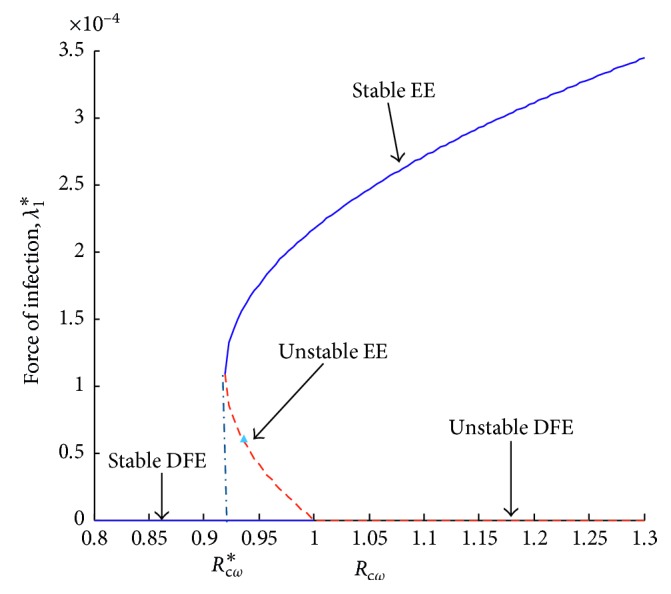
Force of infection, λ₁, versus control reproduction number, R_cw.

3.3.2. Existence of Resistant Influenza Strain Only Endemic State

There exists an endemic state when the resistant strain persists and the wild-type strain dies out. Solving (1) in terms of λ₂ and substituting I_R^∗ into λ₂^∗ yields the following equation:

$$\begin{array}{c}{\lambda }_2\left(-Q_2{Q}_3\left(\mu +\varphi +{\lambda }_2\right)\left(\mu -\left(-1+\epsilon \right){\lambda }_2\right)+\left(\mu +\varphi -\epsilon \varphi -\left(-1+\epsilon \right){\lambda }_2\right)\left(\varphi Q_3\overline{{\beta }_{\text{r}}}+{\alpha }_{\text{r}}\vartheta {\lambda }_2\right)\right)=0.\end{array}$$ (36)

When λ₂=0, resistant influenza-free equilibrium is obtained. The remaining part of polynomial (36) can be expressed as

$$\begin{array}{c}P\left({\lambda }_2\right)=A_2{\lambda }_2^2+A_1{\lambda }_2+A_0,\end{array}$$ (37)

where

$$\begin{array}{c}{A}_2=\left(-1+\epsilon \right)\left(Q_2{Q}_3-{\alpha }_{\text{r}}\vartheta \right),\\ A_1={\alpha }_{\text{r}}\varphi \vartheta \left(\epsilon -1\right)+Q_2{Q}_3\mu \left(1-\epsilon \right)+Q_2{Q}_3\varphi \left(1-\epsilon \right)+Q_3\overline{{\beta }_{\text{r}}}\pi \left(\epsilon -1\right)-{\alpha }_{\text{r}}\mu \vartheta ,\\ A_0=Q_3\left(\mu \left(\mu +\varphi \right)Q_2\left(1-R_{\text{cr}}\right)\right).\end{array}$$ (38)

Using the procedure as in Section 3.3.1, it can be shown that the system exhibits a backward bifurcation when R_cr < 1. This is illustrated by Figure 7.

Figure 7.

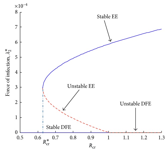
Force of infection, λ₂, versus control reproduction number, R_cr.

4. Sensitivity Analysis

In order to curb the spread of influenza in a given population, it is essential to know the relative importance of the different parameters responsible for its transmission and prevalence. Influenza transmission and endemicity are directly related to R_c. As in [62, 63], the normalized forward sensitivity analysis is used for this model. The normalized sensitivity index which measures the relative change in a parameter k, with respect to the reproduction number R_c is given by P_q=(k/R_c)(∂R_c/∂k), [64]. The sign of P_q determines the direction of changes, increasing (for positive P_q) and decreasing (for negative P_q) [65]. The sensitivity indices of the model reproduction number to the parameters in the model at the parameter values described in Table 2 are calculated. These indices reveal how crucial each parameter is to disease transmission and spread making it possible to discover parameters that have a high impact on R_c and should be targeted by intervention strategies. The calculated sensitivity indices of R_c are given in Table 3.

Table 3.

Sensitivity indices of R_cw and R_cr.

Parameter	Sensitivity index
Sensitivity indices ofR cw
β w	0.99999
π	1
ϕ	−0.2582418982
ε	−2.064509968
α	−0.6094452335
a w	−0.0305027644
b	−0.3599326204
μ	−0.7418774828
Sensitivity indices ofR cr
β r	0.99999
π	1
b	0.02746556942
ϕ	−0.2582418983
ε	−2.064509968
α r	−0.7724001063
a r	−0.2271765018
μ	−0.7421814939

Small variations in a highly sensitive parameter lead to large quantitative changes; hence, caution should be taken when handling such a parameter. A positive sensitivity index indicates that R_c is an increasing function of the corresponding parameter, and hence, an increase in the parameter while other factors are held constant leads to an increase in the reproduction number and could lead to disease spread [65]. On the other hand, a negative sensitivity index shows that an increase in the parameter while other factors are held constant leads to a decrease in the reproduction number, which could then lead to disease control. For instance, if the vaccination rate, ϕ, is increased by 10%, R_c would decrease by about 2.5%. Increasing the recruitment rate by 10% increases the R_c by 10%.

5. Numerical Simulation

5.1. Effects of Drug Resistance

For the parameter values in Table 2, as the drug resistance increases, the changes in the reproduction numbers can be observed as shown in Figure 8.

Figure 8.

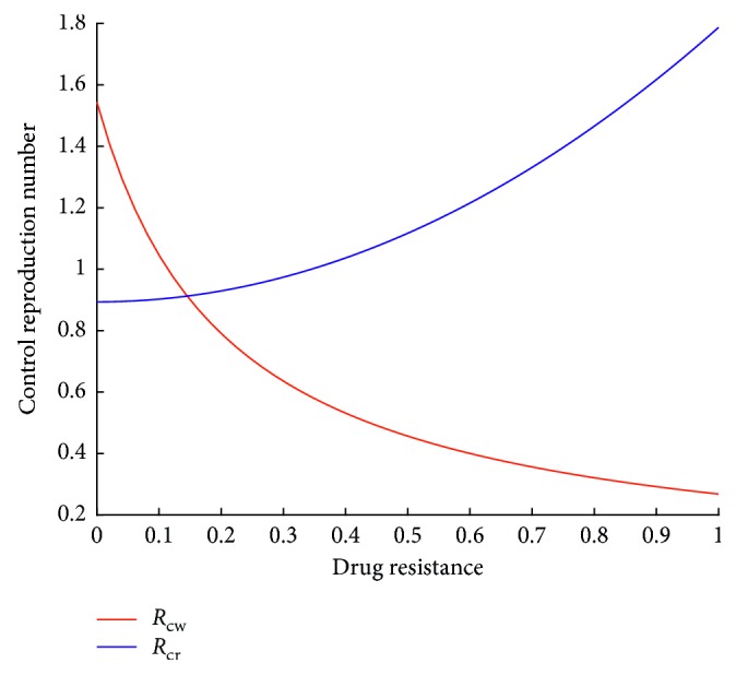
Relationship between reproduction numbers and drug resistance.

In conformity with the expectation, increased drug resistance leads to an increase in R_cr. It can also be observed that R_cw decreases with increased drug resistance. The implication of increased drug resistance on infected population is discussed in the next section.

5.1.1. Effects of Drug Resistance on Infected Population

The rate of drug resistance is varied holding all the other parameter values constant. Figures 9 and 10 are obtained.

Figure 9.

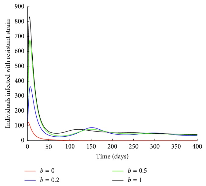
Effect of drug resistance on I_R class.

Figure 10.

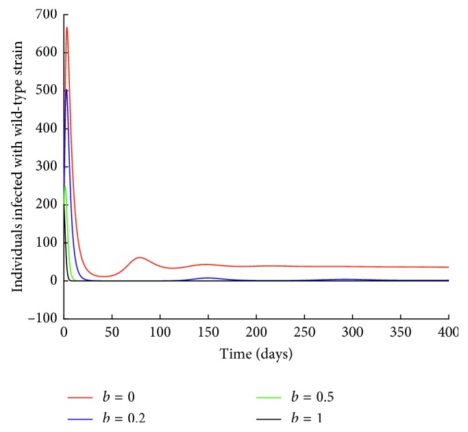
Effect of drug resistance on I_w class.

It can be observed from Figure 9 that when there is no development of drug resistance (b=0), the number of individuals infected with resistant strain decreases to zero. An increase in the rate of drug resistance leads to an increase in the number of individuals infected with resistant strain.

Next, the effect of drug resistance on individuals infected with wild-type strain is investigated.

From Figure 10, it can be observed that an increase in the rate of drug resistance leads to a decrease in the number of individuals infected with wild-type strain. For instance, when b=1, the number of individuals infected with wild-type strain decrease to zero. This could be attributed to the mutation of the wild-type strain to resistant strain.

5.2. Effect of Vaccination on Reproduction Number and on Influenza Prevalence in the Model Population

Figures 11 and 12 show the population dynamics of the infected individuals in a case where there is no vaccination. The reproduction number of the resistant strain is obtained as 2.7762, while that of the wild-type strain is obtained as 3.0288.

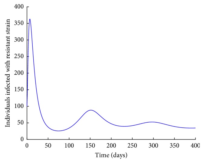
Figure 11.

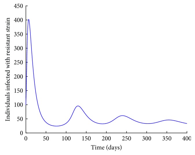
I _R individuals with no vaccination.

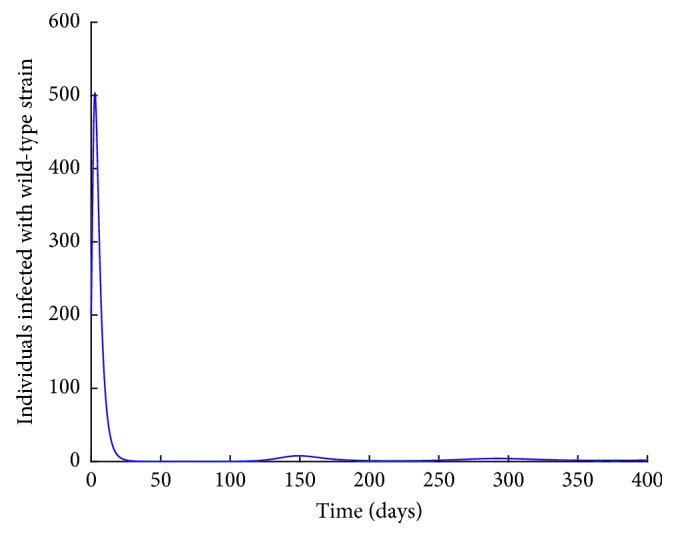
Figure 12.

I _w individuals with no vaccination.

Note that the reproduction number for the two cases is greater than one. It can be observed from Figures 11 and 12 that the resistant strain and the wild-type strain persist in the population.

Next, numerical simulation is done in the case where there is vaccination. Using the parameter values in Table 2, Figures 13 and 14 are obtained. The control reproduction number (17), R_cr, is obtained as 0.9059, and R_cw is obtained as 0.9883.

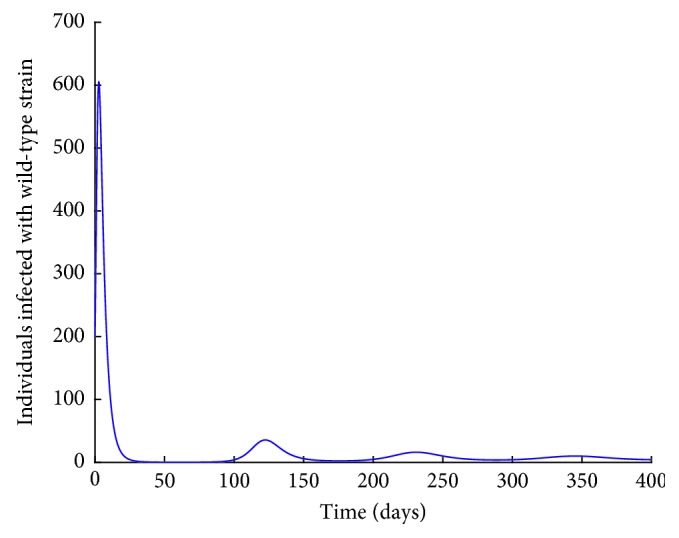
Figure 13.

I _R individuals with vaccination.

Figure 14.

I _w individuals with vaccination.

Note that the reproduction number in this case is less than one. Vaccination reduces the reproduction number. However, from Figures 13 and 14, it can be observed that both the resistant strain and the wild-type strain do not completely die out from the population despite the reproduction number being less than one. These findings are consistent with Figures 6 and 7 obtained in Sections 3.3.1 and 3.3.2, respectively. This shows that bringing the reproduction number below unity does not describe the necessary effort to curb the spread of influenza. Therefore, the intervention strategies should be carefully implemented to bring the reproduction number below the critical value. It can also be observed from Figures 11–14 that the level of persistence of the resistant strain is higher than that of the wild-type strain.

5.3. Effect of Transmission Rates β_w and β_r on Infected Population

5.3.1. Case 1: Effect of β_w on I_w Individuals

From Figure 15, it can be observed that the higher the transmission rate, the higher the number of infected individuals. The number of infected individuals drastically decreases to zero within a short period of time but then starts to increase again shortly after and the disease does not completely die out after that (this is when β_w = 0.002 and 0.0015). When β_w = 0.00095, it can be observed that the number of infected individuals declines to zero and the disease completely dies out. It should be noted that for this case, the R_cw = 0.9205 which is below the critical value R_cw^∗ = 0.9351.

Figure 15.

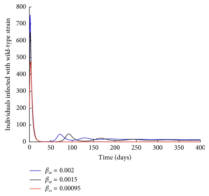
Effect of β_w on individuals infected with wild-type strain.

5.3.2. Case 2: Effect of β_r on I_R Individuals

It is observed from Figure 16 that the higher the transmission rate, the higher the number of infected individuals. It is also interesting to note that when β_r = 0, there still exist individuals infected with the resistant strain and the strain persists in the population. This shows that curbing the spread of the resistant strain is quite difficult. This could be due to the fact that the spread of the resistant strain is fuelled by two processes: transmission and mutation of the wild-type strain to resistant strain.

Figure 16.

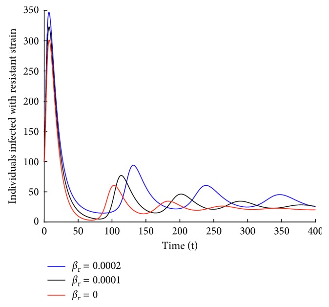
Effect of β_r on individuals infected with resistant strain.

6. Conclusion

To completely wipe out influenza from a population continues to prove difficult. This is because the virus evolves very rapidly and is able to change from one season to the other. This is extensively explained in [3, 7, 9]. Results from our model show that vaccination reduces the reproduction number, and hence, it could be used as a control strategy. However, caution should be taken because influenza can still persist in case there is backward bifurcation. Results also show that it is easier to curtail the spread of the wild-type strain especially in a given season than the resistant strain. This could be through social distancing and issuing travel bans to areas affected with the virus. For the resistant strain, social distancing could also be used as a control strategy in addition to reducing the mutation of the wild-type strain.

Data Availability

The data used to support the findings of this study are included within the article.

Conflicts of Interest

The authors declare that there are no conflicts of interest regarding the publication of this article.

References

- 1.White M. C., Lowen A. C. Implications of segment mismatch for influenza a virus evolution. Journal of General Virology. 2017;99(1):3–16. doi: 10.1099/jgv.0.000989. [DOI] [PMC free article] [PubMed] [Google Scholar]
- 2.Taubenberger J. K., Morens D. M. Influenza viruses: breaking all the rules. mBio. 2013;4(4) doi: 10.1128/mbio.00365-13.e00365-13 [DOI] [PMC free article] [PubMed] [Google Scholar]
- 3.CDC. How the Flu Virus Can Change: Drift and Shift. Atlanta, GA, USA: CDC; 2017. https://www.cdc.gov/flu/about/viruses/change.htm. [Google Scholar]
- 4.Smith G. J., Vijaykrishna D., Bahl J., et al. Origins and evolutionary genomics of the 2009 swine-origin H1N1 influenza a epidemic. Nature. 2009;459(7250):p. 1122. doi: 10.1038/nature08182. [DOI] [PubMed] [Google Scholar]
- 5.WHO. WHO/Europe—Influenza-Data and Statistics. Geneva, Switzerland: WHO; 2017. http://www.euro.who.int/en/health-topics/communicable-diseases/influenza/data-and-statistics. [Google Scholar]
- 6.CDC. Clinical Signs and Symptoms of Influenza: Health Professionals–CDC. Atlanta, GA, USA: CDC; 2017. https://www.cdc.gov/flu/professionals/acip/clinical.htm. [Google Scholar]
- 7.Moscona A. Neuraminidase inhibitors for influenza. New England Journal of Medicine. 2005;353(13):1363–1373. doi: 10.1056/nejmra050740. [DOI] [PubMed] [Google Scholar]
- 8.CDC. Preventing the Flu: Good Health Habits Can Help Stop Germs–CDC. Atlanta, GA, USA: CDC; 2017. https://www.cdc.gov/flu/protect/habits.htm. [Google Scholar]
- 9.Matheka D. M., Mokaya J., Maritim M. Overview of influenza virus infections in Kenya: past, present and future. Pan African medical journal. 2013;14 doi: 10.11604/pamj.2013.14.138.2612. [DOI] [PMC free article] [PubMed] [Google Scholar]
- 10.Cheng K., Leung P. What happened in china during the 1918 influenza pandemic? International Journal of Infectious Diseases. 2007;11(4):360–364. doi: 10.1016/j.ijid.2006.07.009. [DOI] [PubMed] [Google Scholar]
- 11.Goeyvaerts N., Willem L., Van Kerckhove K., et al. Estimating dynamic transmission model parameters for seasonal influenza by fitting to age and season-specific influenza-like illness incidence. Epidemics. 2015;13:1–9. doi: 10.1016/j.epidem.2015.04.002. [DOI] [PubMed] [Google Scholar]
- 12.Saunders-Hastings P. R., Krewski D. Reviewing the history of pandemic influenza: understanding patterns of emergence and transmission. Pathogens. 2016;5(4):p. 66. doi: 10.3390/pathogens5040066. [DOI] [PMC free article] [PubMed] [Google Scholar]
- 13.CDC. Past Pandemics. Atlanta, GA, USA: CDC; 2017. https://www.cdc.gov/flu/pandemic-resources/basics/past-pandemics.html. [Google Scholar]
- 14.WHO. WHO—Influenza. Geneva, Switzerland: WHO; 2017. http://www.who.int/mediacentre/factsheets/2003/fs211/en/ [Google Scholar]
- 15.CDC. Seasonal Flu Death Estimate Increases Worldwide. Atlanta, GA, USA: CDC; 2017. https://www.cdc.gov/media/releases/2017/p1213-flu-death-estimate.html. [Google Scholar]
- 16.Hope-Simpson R. The role of season in the epidemiology of influenza. Epidemiology & Infection. 1981;86(1):35–47. doi: 10.1017/s0022172400068728. [DOI] [PMC free article] [PubMed] [Google Scholar]
- 17.Finkelman B. S., Viboud C., Koelle K., Ferrari M. J., Bharti N., Grenfell B. T. Global patterns in seasonal activity of influenza A/H3N2, A/H1N1, and B from 1997 to 2005: viral coexistence and latitudinal gradients. PLoS One. 2007;2(12) doi: 10.1371/journal.pone.0001296.e1296 [DOI] [PMC free article] [PubMed] [Google Scholar]
- 18.Shek L. P.-C., Lee B.-W. Epidemiology and seasonality of respiratory tract virus infections in the tropics. Paediatric Respiratory Reviews. 2003;4(2):105–111. doi: 10.1016/s1526-0542(03)00024-1. [DOI] [PubMed] [Google Scholar]
- 19.Katz M. A., Schoub B. D., Heraud J. M., Breiman R. F., Njenga M. K., Widdowson M.-A. Influenza in Africa: uncovering the epidemiology of a long-overlooked disease. Journal of Infectious Diseases. 2012;206(1):S1–S4. doi: 10.1093/infdis/jis548. [DOI] [PubMed] [Google Scholar]
- 20.WHO. Influenza. Geneva, Switzerland: WHO; 2017. http://www.who.int/influenza/gisrs_laboratory/updates/summaryreport_20171002/en/ [Google Scholar]
- 21.WHO. Influenza. Geneva, Switzerland: WHO; 2018. http://www.who.int/influenza/gisrs_laboratory/updates/summaryreport/en/ [Google Scholar]
- 22.RGA. Seasonal Influenza and Mortality. St. Louis, MO, USA: RGA; 2018. https://www.rgare.com/knowledge-center/articles/seasonal-influenza-and-mortality. [Google Scholar]
- 23.Ku A., Chan L. The first case of H5N1 avian influenza infection in a human with complications of adult respiratory distress syndrome and Reye’s syndrome. Journal of Paediatrics and Child Health. 1999;35(2):207–209. doi: 10.1046/j.1440-1754.1999.t01-1-00329.x. [DOI] [PubMed] [Google Scholar]
- 24.Hien T. T., Liem N. T., Dung N. T., et al. Avian influenza a (H5N1) in 10 patients in Vietnam. New England Journal of Medicine. 2004;350(12):1179–1188. doi: 10.1056/nejmoa040419. [DOI] [PubMed] [Google Scholar]
- 25.Gao R., Cao B., Hu Y., et al. Human infection with a novel avian-origin influenza a (H7N9) virus. New England Journal of Medicine. 2013;368(20):1888–1897. doi: 10.1056/nejmoa1304459. [DOI] [PubMed] [Google Scholar]
- 26.Mazel-Sanchez B., Boal-Carvalho I., Silva F., Dijkman R., Schmolke M. H5N1 influenza a virus PB1-F2 relieves HAX-1-mediated restriction of avian virus polymerase pa in human lung cells. Journal of Virology. 2018;92(11):p. e00425–18. doi: 10.1128/jvi.00425-18. [DOI] [PMC free article] [PubMed] [Google Scholar]
- 27.Hurtado T. R. Human influenza a (H5N1): a brief review and recommendations for travelers. Wilderness & Environmental Medicine. 2006;17(4):276–281. doi: 10.1580/06-weme-ra-007r.1. [DOI] [PubMed] [Google Scholar]
- 28.Li F., Choi B., Sly T., Pak A. Finding the real case-fatality rate of H5N1 avian influenza. Journal of Epidemiology & Community Health. 2008;62(6):555–559. doi: 10.1136/jech.2007.064030. [DOI] [PubMed] [Google Scholar]
- 29.WHO. Influenza at the Human-Animal Interface. Geneva, Switzerland: WHO; 2018. http://www.who.int/influenza/human_animal_interface/Influenza_Summary_IRA_HA_interface_25_01_2018_FINAL.pdf. [Google Scholar]
- 30.Chen H., Yuan H., Gao R., et al. Clinical and epidemiological characteristics of a fatal case of avian influenza a h10n8 virus infection: a descriptive study. The Lancet. 2014;383(9918):714–721. doi: 10.1016/s0140-6736(14)60111-2. [DOI] [PubMed] [Google Scholar]
- 31.Zhang Z., Li R., Jiang L., et al. The complexity of human infected AIV H5N6 isolated from china. BMC Infectious Diseases. 2016;16(1):p. 600. doi: 10.1186/s12879-016-1932-1. [DOI] [PMC free article] [PubMed] [Google Scholar]
- 32.Huang Y., Li X., Zhang H., et al. Human infection with an avian influenza a (H9N2) virus in the middle region of china. Journal of Medical Virology. 2015;87(10):1641–1648. doi: 10.1002/jmv.24231. [DOI] [PubMed] [Google Scholar]
- 33.Yuan J., Zhang L., Kan X., et al. Origin and molecular characteristics of a novel 2013 avian influenza a (H6N1) virus causing human infection in Taiwan. Clinical Infectious Diseases. 2013;57(9):1367–1368. doi: 10.1093/cid/cit479. [DOI] [PubMed] [Google Scholar]
- 34.Alexander M. E., Bowman C., Moghadas S. M., Summers R., Gumel A. B., Sahai B. M. A vaccination model for transmission dynamics of influenza. SIAM Journal on Applied Dynamical Systems. 2004;3(4):503–524. doi: 10.1137/030600370. [DOI] [Google Scholar]
- 35.Guo D., Li K. C., Peters T. R., Snively B. M., Poehling K. A., Zhou X. Multi-scale modeling for the transmission of influenza and the evaluation of interventions toward it. Scientific Reports. 2015;5(1) doi: 10.1038/srep08980. [DOI] [PMC free article] [PubMed] [Google Scholar]
- 36.Srivastav A. K., Ghosh M. Analysis of a simple influenza a (H1N1) model with optimal control. World Journal of Modelling and Simulation. 2016;12(4):307–319. [Google Scholar]
- 37.Mikolajczyk R., Krumkamp R., Bornemann R., Ahmad A., Schwehm M., Duerr H. Influenza–insights from mathematical modelling. Deutsches Arzteblatt International. 2009;106(47):777–782. doi: 10.3238/arztebl.2009.0777. [DOI] [PMC free article] [PubMed] [Google Scholar]
- 38.Larson E. W., Dominik J. W., Rowberg A. H., Higbee G. A. Influenza virus population dynamics in the respiratory tract of experimentally infected mice. Infection and Immunity. 1976;13(2):438–447. doi: 10.1128/iai.13.2.438-447.1976. [DOI] [PMC free article] [PubMed] [Google Scholar]
- 39.Imran M., Malik T., Ansari A. R., Khan A. Mathematical analysis of swine influenza epidemic model with optimal control. Japan Journal of Industrial and Applied Mathematics. 2016;33(1):269–296. doi: 10.1007/s13160-016-0210-3. [DOI] [PMC free article] [PubMed] [Google Scholar]
- 40.Lee S., Chowell G., Castillo-Chávez C. Optimal control for pandemic influenza: the role of limited antiviral treatment and isolation. Journal of Theoretical Biology. 2010;265(2):136–150. doi: 10.1016/j.jtbi.2010.04.003. [DOI] [PubMed] [Google Scholar]
- 41.Prosper O., Saucedo O., Thompson D., Torres-Garcia G., Wang X., Castillo-Chavez C. Modeling control strategies for concurrent epidemics of seasonal and pandemic H1N1 influenza. Mathematical Biosciences and Engineering. 2011;8(1):141–170. doi: 10.3934/mbe.2011.8.141. [DOI] [PubMed] [Google Scholar]
- 42.Woolhouse M., Farrar J. Policy: an intergovernmental panel on antimicrobial resistance. Nature. 2014;509(7502):555–557. doi: 10.1038/509555a. [DOI] [PubMed] [Google Scholar]
- 43.van der Vries E., Schutten M., Fraaij P., Boucher C., Osterhaus A. Influenza virus resistance to antiviral therapy. Advances in Pharmacology. 2013;67:217–246. doi: 10.1016/B978-0-12-405880-4.00006-8. [DOI] [PubMed] [Google Scholar]
- 44.Li T., Chan M. C., Lee N. Clinical implications of antiviral resistance in influenza. Viruses. 2015;7(9):4929–4944. doi: 10.3390/v7092850. [DOI] [PMC free article] [PubMed] [Google Scholar]
- 45.CDC. About Antimicrobial Resistance—Antibiotic/Antimicrobial Resistance. Atlanta, GA, USA: CDC; 2017. https://www.cdc.gov/drugresistance/about.html. [Google Scholar]
- 46.Hayes J. D., Wolf C. R. Molecular mechanisms of drug resistance. Biochemical Journal. 1990;272(2):p. 281. doi: 10.1042/bj2720281. [DOI] [PMC free article] [PubMed] [Google Scholar]
- 47.Blower S., Aschenbach A., Gershengorn H., Kahn J. Predicting the unpredictable: transmission of drug-resistant HIV. Nature Medicine. 2001;7(9):1016–1020. doi: 10.1038/nm0901-1016. [DOI] [PubMed] [Google Scholar]
- 48.Blower S., Volberding P. What can modeling tell us about the threat of antiviral drug resistance? Current Opinion in Infectious Diseases. 2002;15(6):609–614. doi: 10.1097/00001432-200212000-00009. [DOI] [PubMed] [Google Scholar]
- 49.Ison M. G., Gubareva L. V., Atmar R. L., Treanor J., Hayden F. G. Recovery of drug-resistant influenza virus from immunocompromised patients: a case series. Journal of Infectious Diseases. 2006;193(6):760–764. doi: 10.1086/500465. [DOI] [PubMed] [Google Scholar]
- 50.Kamali A., Holodniy M. Influenza treatment and prophylaxis with neuraminidase inhibitors: a review. Infection and Drug Resistance. 2013;6:p. 187. doi: 10.2147/IDR.S36601. [DOI] [PMC free article] [PubMed] [Google Scholar]
- 51.CDC. Influenza Antiviral Drug Resistance. Atlanta, GA, USA: CDC; 2017. https://www.cdc.gov/flu/about/qa/antiviralresistance.htm. [Google Scholar]
- 52.Hayden F. G., de Jong M. D. Emerging influenza antiviral resistance threats. Journal of Infectious Diseases. 2011;203(1):6–10. doi: 10.1093/infdis/jiq012. [DOI] [PMC free article] [PubMed] [Google Scholar]
- 53.Lipsitch M., Cohen T., Murray M., Levin B. R. Antiviral resistance and the control of pandemic influenza. PLoS Medicine. 2007;4(1):p. e15. doi: 10.1371/journal.pmed.0040015. [DOI] [PMC free article] [PubMed] [Google Scholar]
- 54.Jnawali K., Morsky B., Poore K., Bauch C. T. Emergence and spread of drug resistant influenza: a two-population game theoretical model. Infectious Disease Modelling. 2016;1(1):40–51. doi: 10.1016/j.idm.2016.07.003. [DOI] [PMC free article] [PubMed] [Google Scholar]
- 55.McCaw J. M., Wood J. G., McCaw C. T., McVernon J. Impact of emerging antiviral drug resistance on influenza containment and spread: influence of subclinical infection and strategic use of a stockpile containing one or two drugs. PLoS One. 2008;3(6) doi: 10.1371/journal.pone.0002362.e2362 [DOI] [PMC free article] [PubMed] [Google Scholar]
- 56.Ferguson N. M., Mallett S., Jackson H., Roberts N., Ward P. A population-dynamic model for evaluating the potential spread of drug-resistant influenza virus infections during community-based use of antivirals. Journal of Antimicrobial Chemotherapy. 2003;51(4):977–990. doi: 10.1093/jac/dkg136. [DOI] [PubMed] [Google Scholar]
- 57.Stilianakis N. I., Perelson A. S., Hayden F. G. Emergence of drug resistance during an influenza epidemic: insights from a mathematical model. Journal of Infectious Diseases. 1998;177(4):863–873. doi: 10.1086/515246. [DOI] [PubMed] [Google Scholar]
- 58.ISG. Vaccine Efficacy and Effectiveness. Melbourne, VIC, Australia: Influenza Specialist Group; 2017. http://www.isg.org.au/index.php/vaccination/vaccine-efficacy-and-effectiveness/ [Google Scholar]
- 59.CDC. Flu Vaccine Coverage Remains Low This Year. Atlanta, GA, USA: Centers for Disease Control and Prevention; 2017. https://www.cdc.gov/media/releases/2016/p1207-flu-vaccine-coverage.html. [Google Scholar]
- 60.Van den Driessche P., Watmough J. Reproduction numbers and sub-threshold endemic equilibria for compartmental models of disease transmission. Mathematical Biosciences. 2002;180(1):29–48. doi: 10.1016/s0025-5564(02)00108-6. [DOI] [PubMed] [Google Scholar]
- 61.Nishiura H., Chowell G. Mathematical and Statistical Estimation Approaches in Epidemiology. Berlin, Germany: Springer; 2009. The effective reproduction number as a prelude to statistical estimation of time-dependent epidemic trends; pp. 103–121. [Google Scholar]
- 62.Rodrigues H. S., Monteiro M. T. T., Torres D. F. M. Sensitivity analysis in a dengue epidemiological model. Conference Papers in Science. 2013;2013:7. doi: 10.1155/2013/721406.721406 [DOI] [Google Scholar]
- 63.Chitnis N., Hyman J. M., Manore C. A. Modelling vertical transmission in vector-borne diseases with applications to rift valley fever. Journal of Biological Dynamics. 2013;7(1):11–40. doi: 10.1080/17513758.2012.733427. [DOI] [PMC free article] [PubMed] [Google Scholar]
- 64.Hategekimana F., Saha S., Chaturvedi A. Dynamics of amoebiasis transmission: stability and sensitivity analysis. Mathematics. 2017;5(4):p. 58. doi: 10.3390/math5040058. [DOI] [Google Scholar]
- 65.Chowell G., Hyman J. M. Mathematical and Statistical Modeling for Emerging and Re-emerging Infectious Diseases. Berlin, Germany: Springer; 2016. [Google Scholar]
Associated Data
This section collects any data citations, data availability statements, or supplementary materials included in this article.
Data Availability Statement