Deep Learning based Classification for Head and Neck Cancer Detection with Hyperspectral Imaging in an Animal Model

Abstract

Hyperspectral imaging (HSI) is an emerging imaging modality that can provide a noninvasive tool for cancer detection and image-guided surgery. HSI acquires high-resolution images at hundreds of spectral bands, providing big data to differentiating different types of tissue. We proposed a deep learning based method for the detection of head and neck cancer with hyperspectral images. Since the deep learning algorithm can learn the feature hierarchically, the learned features are more discriminative and concise than the handcrafted features. In this study, we adopt convolutional neural networks (CNN) to learn the deep feature of pixels for classifying each pixel into tumor or normal tissue. We evaluated our proposed classification method on the dataset containing hyperspectral images from 12 tumor-bearing mice. Experimental results show that our method achieved an average accuracy of 91.36%. The preliminary study demonstrated that our deep learning method can be applied to hyperspectral images for detecting head and neck tumors in animal models.

1. INTRODUCTION

Although the overall incidence of cancer has declined in the United States within the past 20 years, there has been a marked increase in the incidence of oropharyngeal cancer (base of tongue and, to a lesser extent, tonsilar) over the same period in both America and Europe [1]. More than a million patients are diagnosed each year with squamous cell carcinoma of the head and neck (HNSCC) worldwide [2]. Hence, early detection and treatment of head and neck cancer are crucially important to improve survival and quality of life for the patients.

Hyperspectral imaging (HSI) is a relatively new technology for obtaining both spatial and spectral information from an object. It has exhibited potential in the diagnosis of head and neck cancer [3–8]. Computer assisted detection and quantitative analysis methods were proposed to detect cancer. Liu et al [3] used the sparse representation for the tongue tumor detection. Lu et al [6, 7] validated a spectral-spatial classification framework based on tensor modeling for head and neck cancer detection with HSI. This method characterized both spatial and spectral properties of the hypercube and effectively performed dimensionality reduction. Chung et al [8] proposed a method based on superpixels, principal component analysis (PCA), and support vector machine (SVM) to distinguish regions of tumor from healthy tissue. However, HSI generates large amount of high dimensional data, it is important to learn the latent feature representation from these high dimensional data. One major limitation of those methods is that they used the handcrafted features, and those features are incapable of adapting to data at hand. Deep learning can automatically learn effective feature hierarchies from the existing data and thus may be able to overcome the limitation.

In this paper, we introduce a deep learning-based modeling framework for the analysis of hyperspectral images for the detection of head and neck cancer in an animal model. We use the convolutional neural networks (CNN) to learn the deep feature from high dimensional data and classify the pixels into tumor and healthy tissue.

2. METHOD

The proposed deep learning based classification method contains three parts: pre-processing, patch extraction, convolutional neural networks (CNN) based training, and post-processing. Figure 1 shows the overview of the method.

Figure 1.

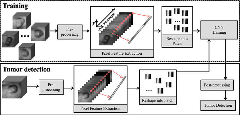
Overview of the proposed deep learning method for cancer detection with hyperspectral imaging.

2.1. Pre-processing

Hyperspectral data preprocessing includes the normalization to eliminate the influence of the dark current. A standard reference white reference was placed in the scene of imaging for the acquisition of the white reference image. The camera shutter was closed during the acquisition of the dark reference image. The data were normalized using the following equation:

$$I\left(\lambda \right)=\frac{I_{raw}\left(\lambda \right)-I_{dark}\left(\lambda \right)}{I_{white}\left(\lambda \right)-I_{dark}\left(\lambda \right)},$$ (1)

where I(λ) is the calculated normalized reflectance value for the wavelength λ, I_raw(λ) is the raw image at the wavelength λ, the I_white(λ) and I_dark(λ) are the corresponding white and dark reference images at the same wavelength.

2.2. Patch extraction

Hyperspectral data consist of hundreds of gray-scale images acquired at different wavelengths. The intensity of each pixel over each spectral band forms a spectral feature. We reshape the spectral feature vector into a patch as the feature of the pixel for training. Since we have 251 spectral bands, we combine the spectral feature vector with a zero vector to obtain a 256-dimension feature vector and reshape it into a 16×16 patch.

2.3. CNN classification

We adopt the convolutional neural networks (CNN) for learning the feature representation of each block and classify it into tumor or normal tissue. CNN is a hierarchical machine learning model [9]. They are made up of neurons that have learnable weights and biases. The input of CNN is a 16×16 patch and the output is the category: tumor or normal tissue. The CNN configuration is shown in Figure 2. The CNN consists of two consecutive convolutional layers and mean-pooling layers. The first and second convolutional layer consists of 12 kernels with the size of 5×5×1, 24 kernels with the size of 3×3×12, respectively. The two layers produce the output, 12 blocks of 12×12 (denoted as 12@12×12) and 24 blocks of 4×4, respectively. The mean-pooling layers are followed by the convolutional layers. It can output the mean values in non-overlapping windows with the size of 2×2 and the stride with 2. So, it cuts the patches into half. The last layer is a fully connected layer with 96 neurons.

Figure 2.

The configuration of the convolutional neural networks (CNN).

2.4. Post-processing

Since our CNN based classification is a pixel based classification, the segmentation result contains noise and holes. We use the morphology operation for the post processing. We use the dilation operation to expand the segmented object and the erosion operation to shrink the segmented object toward a regular shape. We use the flood-fill operation to fill holes in the segmented binary image. Finally, we find the biggest connected component as our detected object.

2.5. Evaluation metrics

The performance of the algorithm is evaluated by the commonly used three measurements: sensitivity, specificity, and accuracy [10–13]. Sensitivity measures the proportion of tumor pixels which are correctly identified as the tumor. Specificity measures the proportion of normal pixels which are correctly identified as normal tissue. They are calculated by:

$$\begin{gathered} Sensitivity=\frac{TP}{TP+FN,} \\ Specificity=\frac{TN}{FP+TN} \end{gathered}$$ (2)

where TP, TN, FP, FN is the number of true positive, true negative, false positive, and false negative, respectively. “True positive” means that the tumor pixels are correctly classified as the tumor. If a tumor pixel is classified as a normal tissue incorrectly, we call it “false negative”. The meanings of “true negative” and “false positive” are defined similarly. The accuracy is an overall measurement of classification performance. It is the ratio of the number of correctly classified examples to the number of all examples. It is calculated by

$$Accuracy=\frac{TP+TN}{TP+FP+TN+FN}.$$ (3)

3. EXPERIMENTS

3.1. Animal model

A head and neck tumor xenograft model was used in our hyperspectral imaging experiment and the HNSCC cell line M4E (doubling rate: ~ 36 hours) was used to initiate the tumor. The M4E cells were maintained as a monolayer culture in Dulbecco’s modified Eagle’s medium (DMEM)/F12 medium (1:1) supplemented with 10% fetal bovine serum (FBS). M4E cells with green fluorescence protein (GFP), which were generated by transfection of pLVTHM vector into M4E cells, were maintained in the same condition as M4E cells. Animal experiments were approved by the Animal Care and Use Committee of Emory University. Female mice aged 4–6 weeks were injected with 2 × 10⁶ M4E cells with GFP on the back of the animals. Hyperspectral images were obtained about two weeks’ post cell injection.

3.2. Database

We acquired the hyperspectral reflectance images from 12 tumor-bearing mice using a CRI Maestro in-vivo imaging system. The system uses a Cermax-type, 300-Watt, Xenon light source. The wavelength setting was defined within the range of 450–950 nm with 2 nm increments. The reflectance images contain 251 spectral bands. The data cube collected is an array of the size 1040 × 1392 × 251. The region of interest (ROI) selected was of the dimension 435 × 390 × 251. The GFP fluorescence images were also acquired as the gold standard for the evaluation of cancer cell detection. Further details can be referred in the previous paper [7].

We conducted leave-one-out cross-validation experiments for the cancer detection in hyperspectral images. We take each hyperspectral image as the testing sample. We randomly select one sample from the 11 remaining samples as the validation set for parameter setting, and the 10 remaining samples as the training set.

3.3. Parameter tuning

The performance of CNN learning could be affected by its different hyperparameter setting. The hyperparameters contain the learning rate, batch size, and number of epochs. To achieve efficient learning, we test the effect of these parameters on the validation set and choose the best ones.

Learning rate

Although a higher learning rate may decay the loss faster, it may not give the best optimization. We test ten numbers for the learning rate from 0.1 to 1.0 with a step size of 0.1 and record the accuracy in Figure 3. Note that we set the epochs to be fixed as 1 and the batch size be fixed as 50. We then choose the best learning rates with the highest accuracy for different mice and use the learning rates in all the following experiments.

Figure 3.

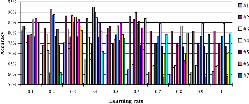
The accuracy in the leave-one-out experiment with different learning rates (from 0.1 to 1), a fixed batch size of 50, and a fixed epoch. Twelve mouse data (#1–12) was used in this experiment.

Batch size

The batch size is the number of samples which are fed at once to the network. We test ten numbers from 10 to 100 with a step size of 10. We record the accuracy under the condition of a fixed learning rate of 1 and one epoch. The results are shown in Figure 4. We identify the best batch size for different mice which contributed to the highest accuracy and use them in all the following experiments.

Figure 4.

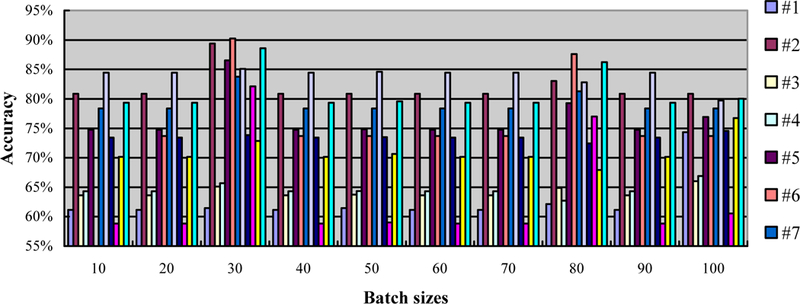
The accuracy in the leave-one-out experiment with different batch sizes (from 10 to 100), a fixed learning rate of 1, and a fixed epoch. Twelve mouse data (#1–12) was used in this experiment.

Number of epochs

The parameter epochs measure how many times every sample has been used during the training process. For example, one epoch means that each sample has been used once. We test ten numbers from 1 to 10 with a step size of 1, and record the accuracy, as shown in Figure 5. To evaluate the effect of epochs, we fix the learning rate to be 1 and the batch size to be 50. Similarly, we choose the best epochs that produce the highest accuracy.

Figure 5.

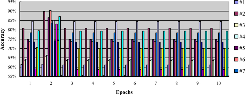
The accuracy in the leave-one-out experiment with different epochs (from 1 to 10), a fixed learning rate of 1, and a fixed batch size of 50. Twelve mouse data (#1–12) was used in this experiment.

3.4. Qualitative results

We show the qualitative results of cancer detection on three mice in Figure 6. Our method can detect the location of the tumor and achieve satisfactory results.

Figure 6.

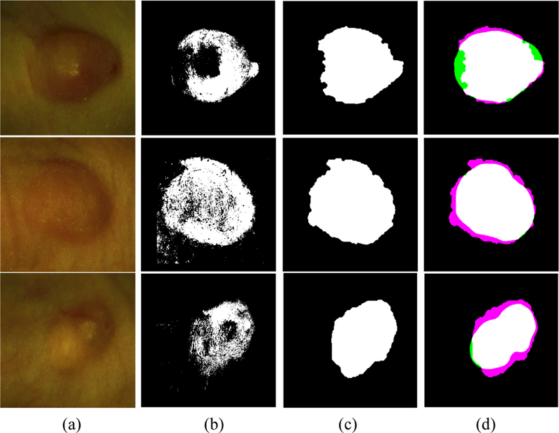
Qualitative evaluation for the detection of head and neck cancer in three mice. (a) RGB composite images generated from the tumor hypercube, (b) The detection results by the CNN based classification, (c) The final results refined by post-processing, and (d) the pair overlap between our detected result and the gold standard from the GFP images, where the white, black, pink, and green regions mean the true positive, true negative, false positive, and false negative regions, respectively.

3.5. Quantitative results

Table 1 provides the quantitative evaluation results of our proposed method for 12 mice. Our method can obtain an average sensitivity of 86.05%, specificity of 93.36%, and accuracy of 91.36%.

Table. 1.

The performance of the cancer detection in 12 tumor-bearing mice.

Mouse ID	Sensitivity (%)	Specificity (%)	Accuracy (%)
1	94.61	97.16	96.63
2	99.40	85.63	90.98
3	92.37	97.01	96.13
4	96.69	91.02	93.08
5	64.53	90.79	81.42
6	99.71	93.39	94.99
7	90.28	97.48	95.58
8	71.01	96.75	91.19
9	97.89	94.19	94.77
10	44.51	92.94	80.07
11	82.14	97.18	90.99
12	99.41	86.76	90.54
Mean	86.05	93.36	91.36
Std	17.47	4.12	5.42

4. CONCLUSION

In this paper, we proposed a deep learning classification method for hyperspectral images for the detection of head and neck cancer in an animal model. The method uses CNN to learn the deep feature from hyperspectral images. As a supervised layerwise training method, the deep neural network can use the 2D structure of an input image to improve the classification performance. The proposed method was able to distinguish between tumor and normal tissue with satisfactory results in this initial experiment. The experimental results demonstrated that our deep learning method is effective for tumor detection in an animal model. Our future work is to test the method in large samples.

REFERENCES

- [1].Mehanna H, et al. , “Prevalence of human papillomavirus in oropharyngeal and nonoropharyngeal head and neck cancer—systematic review and meta analysis of trends by time and region,” Head & neck, 35(5), 747–755 (2013). [DOI] [PubMed] [Google Scholar]
- [2].Haddad RI and Shin DM, “Recent advances in head and neck cancer,” New England Journal of Medicine, 359(11), 1143–1154 (2008). [DOI] [PubMed] [Google Scholar]
- [3].Liu Z, Wang H, and Li Q, “Tongue tumor detection in medical hyperspectral images,” Sensors, 12(1), 162–174 (2011). [DOI] [PMC free article] [PubMed] [Google Scholar]
- [4].Roblyer D, et al. , “Multispectral optical imaging device for in vivo detection of oral neoplasia,” Journal of biomedical optics, 13(2), 024019–024019 (2008). [DOI] [PMC free article] [PubMed] [Google Scholar]
- [5].Roblyer D, et al. “In vivo fluorescence hyperspectral imaging of oral neoplasia,” in SPIE BiOS, Biomedical Optics International Society for Optics and Photonics, 71690J–71690J (2009). [Google Scholar]
- [6].Lu G, et al. “Spectral-spatial classification using tensor modeling for cancer detection with hyperspectral imaging,” in SPIE Medical Imaging, International Society for Optics and Photonics, 903413–903413 (2014). [DOI] [PMC free article] [PubMed] [Google Scholar]
- [7].Lu G, et al. “Spectral-spatial classification for noninvasive cancer detection using hyperspectral imaging,” Journal of biomedical optics, 19(10), 106004–106004 (2014). [DOI] [PMC free article] [PubMed] [Google Scholar]
- [8].Chung H, et al. “Superpixel-based spectral classification for the detection of head and neck cancer with hyperspectral imaging,” in SPIE Medical Imaging, International Society for Optics and Photonics, 978813–978813 (2016). [DOI] [PMC free article] [PubMed] [Google Scholar]
- [9].Krizhevsky A, Sutskever I, and Hinton GE. “Imagenet classification with deep convolutional neural networks,” in Advances in neural information processing systems, 1097–1105 (2012).
- [10].Fei B, et al. , “MR/PET quantification tools: Registration, segmentation, classification, and MR-based attenuation correction,” Medical physics, 39(10), 6443–6454 (2012). [DOI] [PMC free article] [PubMed] [Google Scholar]
- [11].Akbari H, Fei B “3D ultrasound image segmentation using wavelet support vector machines,” Medical physics, 39(6), 2972–2984 (2012). [DOI] [PMC free article] [PubMed] [Google Scholar]
- [12].Yang X, Wu S, Sechopoulos I, and Fei B “Cupping artifact correction and automated classification for high-resolution dedicated breast CT images,” Medical physics, 39(10), 6397–6406 (2012). [DOI] [PMC free article] [PubMed] [Google Scholar]
- [13].Wang H, and Fei B “An MR image-guided, voxel-based partial volume correction method for PET images,” Medical physics, 39(1), 179–194 (2012). [DOI] [PMC free article] [PubMed] [Google Scholar]