

Abstract
Transcranial electric stimulation (TES) is an increasingly popular method for non-invasive modulation of brain activity and a potential treatment for neuropsychiatric disorders. However, there are concerns about the reliability of its application because of variability in TES-induced intracranial electric fields across individuals. While realistic computational models offer can help to alleviate these concerns, their direct empirical validation is sparse, and their practical implications are not always clear. In this study, we combine direct intracranial measurements of electric fields generated by TES in surgical epilepsy patients with computational modeling. First, we directly validate the computational models and identify key parameters needed for accurate model predictions. Second, we derive practical guidelines for a reliable application of TES in terms of the precision of electrode placement needed to achieve a desired electric field distribution. Based on our results, we recommend electrode placement accuracy to be < 1cm for a reliable application of TES across sessions.
Introduction
Transcranial electric stimulation (TES), including transcranial direct current (tDCS) or alternating current (tACS) stimulation, is an increasingly popular method for non-invasive modulation of neural activity in humans (Paulus, 2011). Typically, weak electric currents (e.g. 1mA) are passed through two or more electrodes attached to the scalp creating a low amplitude electric field in the brain. Repeat administration of these currents is increasingly considered as a potential therapeutic modality for psychiatry due to the ability to produce sustained changes in neural function, possibly by inducing neuroplastic changes (Kuo et al., 2014). As TES moves towards the clinical realm, the need for consistent, reliable administration of TES across sessions and individuals becomes increasingly important.
A common practice in the application of TES is to equate the placement of electrodes across individuals using anatomical landmarks defined using a reference system, such as the International 10–20 system (Woods et al., 2016). However, intracranial electric field measurements have shown that the spatial distribution of the electric fields (including orientation and strength) during TES can have intricate patterns (Huang et al., 2017; A. Opitz et al., 2016), which significantly increases the difficulty of creating reliable stimulation protocols. In this regard, current practices tend to rely on consistent placement of reference systems for the identification of anatomical landmarks to guide the targeting of stimulation; however, there have been only limited efforts to establish acceptable tolerance limits for variation in placement across administrations.
Realistic computational models of the brain offer a potential solution for increasing the spatial accuracy of targeting for stimulation. In addition to accounting for the impact of the expected variations in anatomy among individuals, they provide a medium for making predictions about the influences of anatomical factors that can vary across the lifespan, or can be affected by disease processes (e.g., Alzheimer’s disease). Examples of such factors include gyral folding, CSF thickness, and skull composition (Opitz et al., 2015). Additionally, they can provide insights into the impact of commonly overlooked technical factors, such as skin conductance and electrode size (Saturnino et al., 2015). Researchers are increasing the use of realistic brain models to devise electrode montages, and to interpret variations in TES outcomes within and across studies investigating differences in electric field spread and strength across individuals (Laakso et al., 2015).
Here, we leverage individual-specific realistic brain models to inform our understanding of variations in the electric field generated by differences in electrode placement from administration to administration, and generate practical guidelines for decreasing this variability. We: a) carry out a validation for the specific realistic brain modeling framework used in the present work; this work confirms the findings of an initial validation effort recently carried out in ten neurosurgical patients (Huang et al., 2017) and extends it to provide an understanding of the impact of skull defects and surgical materials on findings, and b) use the validated model to establish estimates of the tolerance limits for the placement of electrodes; tolerance is determined with respect to the consistency of the spatial distribution of the electric field and that of the electric field strength generated. This allows us to derive an estimate of the minimal accuracy needed for electrode placement to reliably administer targeted transcranial electrical stimulation.
Methods
Participants.
Model Validation.
Experimental data was obtained from a 29-year-old male patient and a 35-year old female patient with refractory epilepsy who underwent presurgical monitoring at North Shore University Hospital. The experimental protocol was approved by the Institutional Review Board of the Feinstein Institute for Medical Research; the patients gave informed consent in accordance with the ethical standards of the Declaration of Helsinki and monitored by the local Institutional Review Board. Generalization to neurotypical participants. To generalize findings from the patient, anatomical MR data from 25 participants of the Human Connectome Project were used to create individual realistic FEM models.
Electrode Placement.
The male patient was implanted with left subdural grid, strip, and depth electrodes (Integra Lifesciences Corp.). The female patient was implanted with bilateral s-EEG electrodes (Adtech Medical Instrument Corp.). The number and placement of electrodes were determined solely by clinical requirements. Electrode positions were identified on a postimplantation CT scan and registered in a two-step procedure - first to the post-implantation MR and then to the pre-implantation MR. The patients were monitored until sufficient data was collected to identify the seizure focus for 8 days. Continuous intracranial video-EEG monitoring was performed with standard recording systems (XLTEK EMU 128 LTM System) with a sampling rate of 500 Hz.
Transcranial Electrical Stimulation.
TES measurements for model validation were conducted in a single session for each patient. Two circular saline-soaked sponge electrodes (25cm2 surface area) were attached to the scalp over the left and right temple (bilateral montage). The electrode montage was chosen to maximize electric field strength in areas with best coverage of recording contacts. A 1Hz alternating current of 1mA was applied (Starstim, Neuroelectrics) for 2 min with a ramp up/down of 10 s. The locations of stimulation electrodes were recorded with photographs.
In Vivo Field Measurements
The measurement of intracranial electric fields generated by TES is central to model validation. In order to estimate electric fields from the recorded potentials we performed the following analysis steps: From each channel we subtracted the mean voltage over a time interval of 1s preceding stimulation onset to correct for baseline differences between channels and bandpass filtered the recorded voltages between 0.5 Hz and 1.5 Hz. To estimate the electric field strength during TES, we calculated the numerical gradient of the recorded voltages using the symmetric difference quotient. The numerical gradient was calculated along the implanted electrodes at the peak up-phase of the recorded voltages. For the central region covered with grid electrodes two gradients were computed along both grid axes and combined by vector addition. To enhance robustness of the electric field estimates we calculated the mean electric field over five stimulation cycles. The computation of the electric field along the electrodes measures the projection of the electric field along a vector spanned by the contacts.
Data Analysis and Modeling
Realistic Brain Model Generation
To identify those factors that most impact the findings generated using realistic brain models, we created four distinct FEM head models of increasing complexity in multiple steps (see Fig. 1). First, we reconstructed WM, GM, ventricles and skin surfaces from the high-resolution preimplantation T1 using Simnibs (Thielscher et al., 2015; Windhoff et al., 2013). The skull was segmented based on intensity thresholding and manual corrections from the co-registered CT image. Most importantly, the skull reconstruction included small openings present from the surgery (Fig. 1B, upper left panel). The inner skull surface marks the beginning of the CSF and the outer skull surface the transition to the skin. To estimate the effect of accurate skull modeling on the estimation of TES electric fields we created a second skull model in which the skull openings were removed manually in the surface reconstruction (Fig. 1B, upper right panel). In addition, we created a representation of the silastic ECOG grid, which due to its insulating material can affect the measured electric field distribution. The ECOG grid was cut from two sides to better fit it to the brain surface during surgery (Fig. 1B, lower left panel). To estimate the effect these details have on the modeled electric field we created an additional version without cuts (Fig. 1B, lower right panel). From these surface reconstructions we created four tetrahedral based volume meshes with approximately 2.8 million elements each with all different skull/grid combinations (see table 1). FEM model creation was similar for the female patient (see Supplementary Material).
Figure 1:
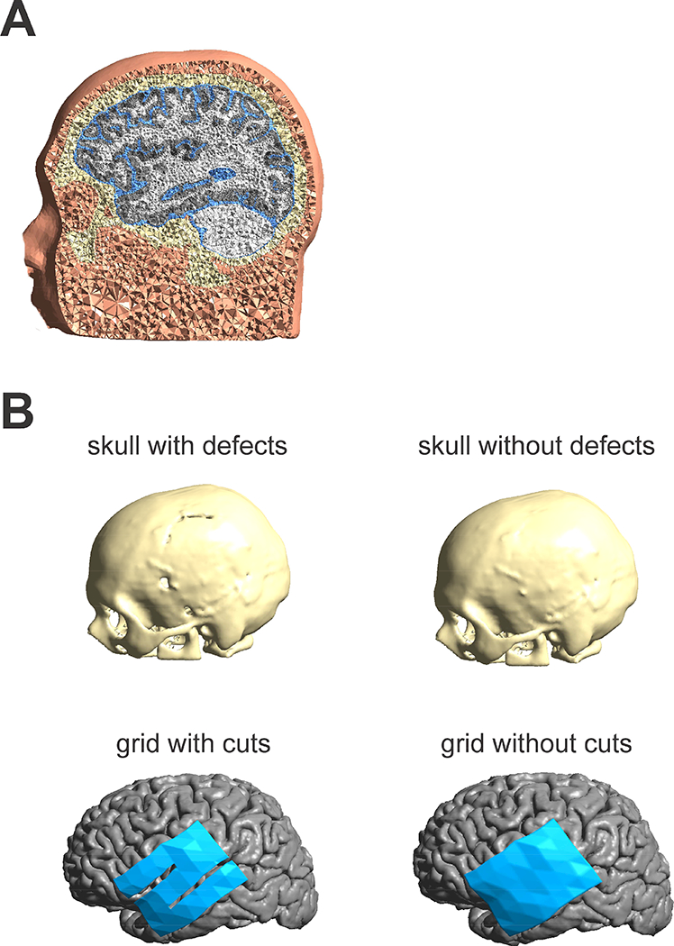
A) Illustration of the FEM head model including scalp, skull, CSF, GM and WM. B) Illustration of four different models investigated. 1. Skull reconstructed from a CT image (upper left). Small skull defects from the surgery were included in the skull model. 2. Skull model with surgical defects closed (upper right). Model with ECOG grid exhibiting small cuts from the surgery (lower left). Model with closed ECOG grid (lower right).
Table 1:
2×2 combinations (skull and grid) employed in the model process resulting in four different FEM models studied.
| Skull/Grid | With grid cuts | Without grid cuts |
| With skull defects | Defects/cuts (Model 1) | Defects/ no cuts (Model 2) |
| Without skull defects | No Defects/cuts (Model 3) | No Defects/no cuts (Model 4) |
FEM simulations
We used the following conductivity values if not specified otherwise 𝜎skin = 0.465 S/m, 𝜎skull= 0.010 S/m, 𝜎CSF =1.654 S/m, 𝜎GM = 0.276 S/m, 𝜎WM = 0.126 S/m and 𝜎grid = 10−10 S/m taken from the literature (Opitz et al., 2015). Other studies have tried to fit conductivity values for different head tissues to achieve best overlap with the measurement data (Huang et al., 2017). This is however a highly underdetermined problem needing more measurement data to reach definitive conclusions. We thus opted to use the standard conductivity values in this study. The conductivity of the skull openings was set to the conductivity of the skin, which was chosen due to the ease of implementation and similar electric properties as the scar tissue. For a qualitatively realistic estimation of the effect of skull defects it is mostly important to model a significantly larger conductivity than the skull in the regions of skull defects (Datta et al., 2010). The electric potential and the electric field were calculated numerically with Simnibs. For details concerning the FEM computations see (Opitz et al., 2015).
Model validation and comparison
In a first analysis, we compared the accuracy of the four different FEM models to predict the measured electric fields, specifically testing for the need of accurate skull and grid modeling in the male patient. For each FEM model we ran 10 simulations changing the grid conductivity from 0.1 S/m to 10−10 S/m. This range of conductivity values was explored to demonstrate the impact of the grid on the electric field with the true conductivity of the grid in the 10−10 S/m range. Thus, our simulations comprise different scenarios from a situation where the grid would have a similar conductivity as the surrounding brain tissues with expected little impact on the electric fields, to a situation where the grid is highly insulating and practically opaque for currents as would occur during the experiment. For the simulated electric fields, we computed their projection along the grid axes to compare them to the measured fields. A more confined analysis was performed for the female patient due to the differences in the implant (see Supplementary Material).
Primary analyses focused on the comparison of measured and modeled values for the electric field strength. It also possible to compare the measured and modelled voltages and directional electric fields as in (Huang et al., 2017, see Supplementary Figure 8). The decision to focus on electric field strength was based on the fact that this is the main variable of interest. Voltages tend to have relatively lower discriminability for model comparisons, with measured and modeled voltages exhibiting very high correlations, irrespective of the exact model chosen; the strength of these relationships is expected, as potentials will always follow a gradient between the stimulation electrodes, irrespective of the exact volume conductor. We further concentrated our analysis on the central grid, which gives relatively high resolution coverage of the area of the cortical surface where the strongest electric fields occur, and this area served as our primary region of interest. To compare measured with modeled electric fields we computed the spatial correlation of the electric field strength across the recording grid between measured and modeled values. Further, we compared the similarity in electric field direction by computing the dot product between the measured and modeled electric field vectors (all normalized to unit length). An aggregate measure of similarity was computed as the sum over all individual contacts.
Effect of stimulation electrode placements
In repeat sessions the location of stimulation electrodes can vary due to procedural shortcomings (e.g. small misalignments during registration) or limited spatial precision in the placement procedure. To study the effect that seemingly small electrode misplacements can have on the achieved electric field, we varied the position of the electrode over the left temple in the computational model; 1cm steps in the anterior-posterior (7 steps) and inferior-superior direction (6 steps) were used, yielding a total of 42 electrode positions (6×7 grid). We focused on this electrode due to its proximity to the recording electrodes and thus potential largest influence on the simulation results in this brain region. This was done for all four head models. The modeled electric field was evaluated at the recording contacts and its projection along the electrode contacts was computed in order to be comparable to the measurement data. During the electric field evaluation, we also slightly varied the location of the grid electrodes on which the modeled electric field would be read out from the mesh. This was done to account for possible slight misalignments between the CT and MR image, which could lead to a spatial uncertainty in the exact grid location. We implemented this by shifting the grid locations in 5mm steps in anterior-posterior and superior-inferior direction (5 steps each with a total of 25 locations).
Translation to neurotypical participants
In order to study how results regarding electrode placement derived from this patient study would translate to normal participants without altered head/brain anatomy, we conducted an additional analysis in a set of 25 healthy participants. Realistic FEM models created for 25 participants from the human connectome dataset (Van Essen et al., 2012) as used in a previous study (Opitz et al., 2016 B) were employed. We repeated the sensitivity analysis towards electrode displacements as for the male patient. For this, we registered the stimulation electrode locations from the patient to the 25 healthy participants and varied the electrode positions on a 6×7 grid (1 cm spacing), calculating a total of 42 FEM simulations for each participant (see Supplementary Fig. 7 for one example). For results to be comparable to the patient scenario, we evaluated electric fields on a virtual grid (projection along grid axes) at the same brain locations as in the patient. We computed spatial correlations of the electric field for each electrode position to the electric field from the central electrode location. This allowed us to estimate to what extent electric fields would change with electrode positions shifted from the central location. We further evaluated the radius in which correlation values would still be up to r = 0.8 compared to the center electrode. For that we up-sampled the correlation grid to determine the area in which correlation values are > 0.8 (Supplementary Fig. 6). In order to confirm that found results are not dependent on the grid resolution we repeated the analysis for one participant with a higher resolution grid (5mm spacing).
Results
Realistic Head Model Validation
The first step in our work was to validate the finite element method approach used to simulate TES electric fields. Specifically, we compared the spatial pattern of the electric field predicted by the realistic head model with the actual electric field measurements obtained from implanted electrodes. To maximize accuracy, the model accounted for the impact of skull defects and the ECOG grid with a realistic conductivity of 10−10 S/m in the model. As depicted in Figure 2, the realistic FEM model successfully approximated the spatial pattern based on the measurement results (Fig. 2 A+B) with a maximum correlation value of r = 0.57 (p < 0.001, Fig. 2C). As would be expected, enhanced electric fields close to the skull defect can be seen in both the measurement and model data. Using recorded voltages or directional electric fields lead to higher correlation values of r = 0.8 (Supplementary Figure 8). Comparable correlation values were found for the female patient (Supplementary Figure 9).
Figure 2:
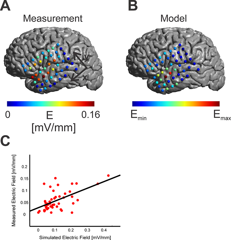
A) Measured absolute electric fields on the cortical surface in mV/mm. A concentration of electrodes with higher electric field strength was found close to the skull defect. B) Simulated electric fields from a realistic head model (skull and grid cuts, grid conductivity, 𝜎grid = 10−10 S/m) resulting in a similar spatial pattern as the measured fields. C) Scatter Plot between simulated electric fields and measured electric fields for each contact. The regression line between simulated and measured electric fields is overlaid in black.
A key question that arises for any realistic head model is how important the varying components modeled are to the end results. While prior work has considered the relative contributions of differing tissue types, the data collected in the present sample provide a unique opportunity to consider the contributions of structural defects and surgical intervention materials. Specifically, we generated a series of models varying whether or not each of these is included. As demonstrated in Figure 3, the failure to account for skull defects significantly degrades the accuracy of the model prediction for the electric field generated. This is demonstrated by the collapse of the correlations for models that do not accurately account for this factor (Fig. 3B, left panel). With decreasing conductivity of the silastic grid and thus increasing opaqueness towards electric currents, only the model that realistically accounts for both the grid and skull leads to high correlations. For realistic grid conductivities of 10−10 S/m we used the R-package cocor (Diedenhofen and Musch, 2015) to statistically test between the different models. Cocor implements a Fisher z-test (Fisher, 1925) to compare the statistical significance in the difference of two correlation values. We tested whether the correlation value between the modeled and measured electric fields were significantly higher for the model accounting for both skull defects and the grid (Model 1) compared to the three other head models. We found the realistic model having significantly higher correlation values (using a Bonferroni corrected p-value of p = 0.0167 as significance threshold) compared to the models not including the skull defects with (z(45) = 3.4859, p = 0.0002, compared to Model 3; z(45) = 2.5730, p = 0.005 compared to Model 4 and z(45) = 0.6312, p = 0.264 compared to Model 2). Furthermore, electric field directions between measured and modeled data were more similar (using a Bonferroni corrected threshold of p= 0.0167) for the model accounting for both skull defect and grid cuts (t(46) = 3.7494, p = 0.0001 compared to Model 4, t(46) = 2.1618, p = 0.018 compared to Model 3 and t(46) = 0.8268, p = 0.21 compared to Model 2, one tailed t-test).
Figure 3:
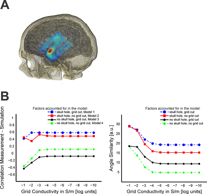
A) Illustration of ECOG grid (with two cuts) in the model with overlaid electric field B) Effect of skull and grid model on the correlation (left panel) between measured and modeled electric fields with varying grid conductivity (S/m in log units) for all four modeled cases (skull hole/ grid cut = blue, skull hole/ no grid cut = red, no skull hole/ no grid cut = green, no skull hole/ grid cut = black). With decreasing conductivity, the grid becomes more opaque to electric currents resulting in shunting around it and affecting the electric fields beneath it. For realistic field estimations, the skull defect needs to be modeled accurately (high correlations only for the models with included skull hole). Only according for grid or skull in a realistic model is not sufficient for realistic predictions. Similarly, the degree of overlap in the direction of measured and modeled electric fields need the skull effects to be accounted for realistically (right panel). Accounting for cuts in the ECOG grid slightly improved the overlap between measured and modeled directions.
Magnitude of the electric field
One notable limitation in the realistic brain model results that was expected based on prior work and merits further investigation, is the magnitude of the predicted electric field measurements. We found that for the male patient the maximum field strength predicted by the model was larger than that we directly measured. Comparing modeled to measured values in absolute terms, we found measurement values to be ~ 40% smaller compared to modeled results for the male patient. The mean electric field strength over all grid contacts was 0.058 mV/mm for the measurement results while the mean electric field strength over the best 50 fitting simulation results was 0.100 mV/mm (range: 0.071 – 0.122 mV/mm). On the other hand, in the female patient, the mean measured electric field strength was 0.115 mV/mm while the mean modelled electric field strength was 0.060 mV/mm, thus underestimating the measured field strength. In understanding the disparity between measured and observed field strengths, it is important to note that conductivities used in the models are largely based on measurements obtained from ex vivo studies; recent work (Huang et al., 2017; Opitz et al., 2017) has questioned the accuracy of these conductivity estimates, outlining the need for future in vivo studies to individually optimize the values used in models.
Establishing Tolerance Limits for Variation in Electrode Placement
Using our validated model, we next examined the impact of variations in electrode placement on the reproducibility of the electric field generated from one administration to the next. A continuous decrease in correlation values is visible as the electrode position moves away from the “optimal” location (Fig. 4). Higher correlation values were found within a radius of about 1cm. Moving farther leads to strongly reduced correlation values. This suggests a minimum accuracy of < 1cm should be achieved in practical experiments in order for models to be meaningful for electrode positioning.
Figure 4:
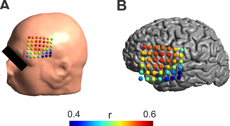
A) Effect of stimulation electrode placements on the correlation between modeled and measured electric fields for the realistic head model (skull and grid cuts, grid conductivity, grid = 10−10 S/m). Colored dots indicate the center of the electrode on the scalp and the associated correlation value between the measured and the modeled electric field. High correlation values were only found in a distance of about 1cm from the maximum. B) The same correlation values as in A) are shown overlaid over the cortical surface.
We further tested the effect of electrode movements in a set of 25 normal participants. This was done to test how far results derived from combined modeling and measurement are applicable in a larger population with non-pathological brain and head anatomy. Similar to the patient results we found that within a 1cm region electric field distributions are highly similar to each other, but quickly decrease within larger electrode movements (Fig. 5). Average correlation values were r = 0.85 and r = 0.6 for 1cm and 2cm distances, comparing the electric field values at the virtual grid locations. Exemplary electric field distributions for various electrode shifts are shown in Supplementary Figure 7. Calculating a radius at which the correlation value would be at r = 0.8 we found a distance of d = 1.15 +- 0.14 cm across all 25 participants. A very similar value (1.124 cm compared to 1.096 cm; less than 5% deviation) was found for the one participant for which electric fields were computed on a high resolution grid (5mm spacing). Investigating the effect of electrode movements on the mean electric field strength showed a less steep drop-off with distance (Supplementary Figure 3). In a supplementary analysis, we estimated the effect of using a very small stimulation electrode (1 cm diameter, contralateral electrode kept identical (5.6 cm diameter) resulting in a more focal electric field distribution. Here we found that correlation values drop off slightly quicker with distance compared to large stimulation electrodes (Supplementary Fig. 4) with a distance of d = 0.95 +- 0.16 for an r = 0.8 threshold. Nevertheless, the basic pattern of electrode movements is very similar for small stimulation electrodes compared to large ones, though there is an increased sensitivity. Based on both patient and healthy subject findings we conclude that electrode placement accuracy of within at least 1cm is required for reliable simulation results. In addition, to the spatial correlation, we also evaluated the effect of changing electric field strength in a region of interest with changing electrode location (see Supplementary Material). Again, we observed a drop-off with increasing distance. For some locations we observed higher field strengths compared to the central location, indicating the importance of individual anatomical factors in determining regions of maximum stimulation (Opitz et al., 2015)
Figure 5:
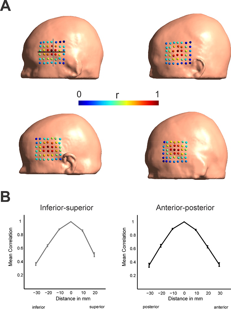
Effect of stimulation electrode placements on the correlation between modeled electric fields in normal participants (n = 4 shown). Colored dots indicate the center of the stimulation electrode on the scalp and the associated correlation value of the electric field distribution to the central electrode (4th row, 4th column). Gray and black lines indicate the electrode locations taken into account to calculate the spatial profiles in B). Effects of electrode movements show high correlations values only in a central region of 1 cm. This suggests for reliable application of TES applications a minimum accuracy in electrode placement < 1cm should be achieved. B) Spatial profiles of correlations with distance to the central electrode along the inferior-superior (gray, left panel) and anterior-posterior direction (black, right panel) as indicated in the first participant in A). Shown are the mean and standard error of the mean across all 25 participants. A drop-off in the correlation values is visible with distance from the central electrode location.
Discussion
The present work leveraged realistic brain models to estimate the consistency of electric field generation across TES administrations as a function of electrode montage placement. The ability of realistic head models to meaningfully predict in vivo measurements of the electric field generated by TES administration in neurosurgical patients was found to be compromised when actual electrode placement differed by more than 1cm. Parametric manipulation of electrode placement in realistic brain models obtained from 25 neurotypical individuals, as well as neurosurgical patients in which in vivo measurements were conducted, converged on 1cm as a limit for error tolerance in the administration of TES across administrations (i.e., sessions). These findings have direct implications for the usage of realistic models to optimize the spatial precision of TES approaches, as well as for protocols relying on repeat administrations of TES over time to ensure sustainable clinical or experimental effects.
Efforts such as the present work are increasingly turning to computational models to make predictions regarding the delivery and dosing of electrical currents to the brain by various transcranial stimulation approaches (e.g., TES, TMS). However, definitive validation of these models has proven challenging due to the need for in vivo measurements, which can only be obtained through invasive electrophysiological recordings. Fortunately, recent work has provided initial validations of the ohmic principles that are believed to govern the conductance of currents generated via TES (Opitz et al., 2016), as well as finite element method based realistic brain models (Huang et al., 2017). Here, we confirm and extend prior validation results for realistic brain models. Similar to prior work, we found that the spatial distribution of the electric field predicted by our realistic brain model was highly correlated with that measured. We further confirm that computational models using current standard conductivities slightly misestimate the measured electric field strength, suggesting the need for individual adjustments of conductivities (Huang et al., 2017). Additionally, we demonstrated a dependency of findings on the accuracy of skull and surgical component modeling. Amongst those investigated, other factors such as gyral folding and CSF thickness have been shown to have a profound effect on TES electric fields (Opitz et al., 2015); these findings emphasize the need for careful consideration individual differences in anatomy especially in populations where they might be altered (e.g. Alzheimer’s). Uncertainties in tissue conductivities (e.g. due to possible neuroinflammation, filling material of skull defects) can affect the accuracy of model predictions. Future efforts to directly measure conductivities could further improve modelling efforts. A related point for future studies will be to determine the amount of model detail, e.g. by including more tissue types (Aydin et al., 2014), that is needed for accurate predictions.
A key output of the present work is the recommendation that electrode montage placement not be allowed to vary by more than 1 cm from a target location. This might seem surprising considering the size of the employed electrode pads. However, the current flow distribution underneath the pads is not homogeneous, but tends to have higher field strengths close to the edges (Suppl. Fig. 7), so that even small shifts result in clearly different field distributions in the brain. In addition to the need for accurate electrode placement, this also emphasizes the importance of an accurate modeling of the electrode pads (Saturnino et al., 2015) for realistic field calculations. Adherence to these recommendations will both affect the ability to use realistic models to improve the spatial precision of TES, and increase the reliability of TES administration across repeat sessions using neuronavigation. This finding is further important for between-subject comparisons due to level of variability (1–2 cm) of brain regions relative to the 10–20 landmarks. Ensuring a reliable application of TES across sessions and individuals is a key prerequisite for meaningful results in TES studies and can help mitigate current concerns about the large observed variability in TES response (López-Alonso et al., 2014; Wiethoff et al., 2014). Another important point is the interpretability of TES effects. If electric fields are delivered inconsistently but effects are observed nevertheless, the results are more difficult to interpret because effects could be driven by other incidentally affected brain regions.
It is important to note that the present work examined the impact of imprecise electrode placement on the delivery of an electric current to the brain, not the neurophysiological or behavioral responses. In addition to these technical factors influencing the physical aspect of TES, a range of physiological factors can affect interindividual variability (Polanía et al., 2018; Ridding and Ziemann, 2010). While this should be examined in future work, it is our belief that a better way forward is for the field is to first develop and adopt criteria for precise administration instead - thereby removing an obvious source of variation that can impact findings within and across individuals.
The present work contributes important novel insights to the larger vision of guiding spatial targeting for transcranial stimulation using computational models. In that regard, there are some limitations of the present work and next steps that merit discussion. First, regarding limitations, it is important to note that the 1cm rule in the present work was established for a two-electrode montage with relatively large electrodes (25 cm2) as well as a second smaller stimulation electrode type. These results can be further extended for other montages and electrode types. Future efforts going beyond electrode montage optimization in single participants are needed to harmonize dosing across participants. While the spatial distribution of the electric field was well approximated by the model, the absolute field strength was overestimated by about 40%. This can be mitigated by adjusting conductivity values of brain tissue which were often acquired ex-vivo (Gabriel et al., 1996) to better match in-vivo field measurements. More direct in-vivo measurements of conductivities in the low frequency domain can help to address the dearth of data in the literature. Efforts to individualize conductivities could be achieved using electric (Cheney et al., 1999) or magnetic resonance electric impedance tomography (Seo, 2003).
With maximum correlation values of r = 0.6, there is still a significant portion of unexplained variance of the data based on the model prediction. One possible reason could be the construction of the head model from the pre-implantation T1-image which differs from the post-implantation T1 with implanted grid electrodes resulting in changes in the brain geometry not fully accounted for by the co-registration procedure. However, it is noteworthy that our main conclusions of the need of accurate skull and grid modeling are not affected by this limitation; i.e., further effects of placement of stimulation electrodes were confirmed in a cohort of neurotypical participants without pathologically altered brain anatomy. Using other metrics of validation can result in correlation of r = 0.8 or higher, demonstrating good overlap.
In sum, we both validated computational models with in-vivo field measurements and derived practical guidelines for their meaningful application. Further, we extended results found in neurosurgical patients to a larger set of neurological typical participants. We conclude that an electrode placement accuracy of at least 1 cm is necessary to ensure a reliable application of TES across sessions. Future efforts to individualize conductivities can further help to harmonize dosing across participants.
Supplementary Material
Supplementary Figure 1: Comparison of measured and modeled electrode field strength for all four investigated head models. The model with skull hole and grid cut resembles the measured data most closely.
Supplementary Figure 2: Comparison of measured and modeled electrode field direction for all four investigated head models. In the measured data, electric field lines converge to a central region beneath the skull defect. This effect is most closely captured by the model including both skull hole and grid cut.
Supplementary Figure 3: Effect of stimulation electrode placements on the electric field strength between modeled electric fields in normal participants (n = 4 shown). Colored dots indicate the center of the stimulation electrode on the scalp and the associated mean electric field strength normalized to the mean electric field strength of the central electrode (4th row, 4th column). Values larger than 1 mean that the mean electric field exceeds the one from the central electrode. B) Spatial profiles of mean electric field strengths with distance to the central electrode along the inferior-superior (gray, left panel) and anterior-posterior direction (black, right panel) as indicated in the first participant in A). Shown are the mean and standard error of the mean across all 25 participants. The results show a decrease in electric field strength with distance from the central electrode, however with a tendency for higher electric field strengths for superior and posterior electrode locations.
Supplementary Figure 4: Effect of stimulation electrode placements on the correlation between modeled electric fields in normal participants (n = 4 shown) using small stimulation electrodes (diameter = 1cm). Colored dots indicate the center of the stimulation electrode on the scalp and the associated correlation value of the electric field distribution to the central electrode (4th row, 4th column). Gray and black lines indicate the electrode locations taken into account to calculate the spatial profiles in B). Effects of electrode movements show high correlations values only in a circumscribed central region. B) Spatial profiles of correlations with distance to the central electrode along the inferior-superior (gray, left panel) and anterior-posterior direction (black, right panel) as indicated in the first participant in A). Shown are the mean and standard error of the mean across all 25 participants. A drop-off in the correlation values is visible with distance from the central electrode location. As expected this drop-off is steeper than using large stimulation electrodes which indicates a higher sensitivity to electrode movements.
Supplementary Figure 5: Effect of stimulation electrode placements on the electric field strength between modeled electric fields in normal participants (n = 4 shown) using small stimulation electrode (diameter = 1cm). Colored dots indicate the center of the stimulation electrode on the scalp and the associated mean electric field strength normalized to the mean electric field strength of the central electrode (4th row, 4th column). Values larger than 1 mean that the mean electric field exceeds the one from the central electrode. B) Spatial profiles of mean electric field strengths with distance to the central electrode along the inferior-superior (gray, left panel) and anterior-posterior direction (black, right panel) as indicated in the first participant in A). Shown are the mean and standard error of the mean across all 25 participants. The results show a decrease in electric field strength with distance from the central electrode, however with a tendency for higher electric field strengths for superior and posterior electrode locations. Compared to the larger stimulation electrodes electric field strength drops off stronger with distance to the central electrode region.
Supplementary Figure 6: A) Spatial grid (6 × 7) with correlation values for each electrode position for one example participant. B) Up-sampled grid from A). C) Area of region (red) with correlation values r > 0.8.
Supplementary Figure 7: Modeled electric field distribution for one example healthy participant showing the effect of movements of the stimulation electrode (25cm2) for all 42 (6×7) stimulation positions. The electric field maximum moves with the electrode from posterior to anterior and inferior to superior, respectively.
Supplementary Figure 8: Effect of different evaluation metrics on the relationship between modelled and measured values. All results shown are based on the realistic head model (skull and grid cuts, grid conductivity, σgrid = 10−10 S/m). A) Correlation between modelled and measured electric field values along the x-grid direction (see Fig. 2) for varying stimulation electrode locations. Colored dots indicate the center of the electrode on the scalp and the associated correlation value between the measured and the modeled electric field. B) Correlation between modelled and measured electric field values along the σ-grid direction for varying stimulation electrode locations. C) Correlation values between modelled and measured absolute electric field values. D) Correlation values between modelled and measured voltages.
Supplementary Figure 9: FEM validation and effect of electrode movements in the second patient. A) Correlation between modelled and measured electric field values along the direction of s-EEG electrodes for varying stimulation electrode locations. B) Correlation values between modelled and measured absolute electric field values.
Acknowledgements
Supported by MH110217, MH111439, pilot funding from NKI and the MnDRIVE Initiative. Transcranial electrical stimulation devices were obtained through an equipment award provided to NKI by the Child Mind Institute (1FD2013–1).
Footnotes
Financial Disclosures
A.O. is an inventor on patents and patent applications describing methods and devices for noninvasive brain stimulation. EY, AT, CS, AM, MM have no conflict of interest.
This is a PDF file of an unedited manuscript that has been accepted for publication. As a service to our customers we are providing this early version of the manuscript. The manuscript will undergo copyediting, typesetting, and review of the resulting proof before it is published in its final citable form. Please note that during the production process errors may be discovered which could affect the content, and all legal disclaimers that apply to the journal pertain.
References
- Aydin Ü, Vorwerk J, Küpper P, Heers M, Kugel H, Galka A, Hamid L, Wellmer J, Kellinghaus C, Rampp S, Wolters CH, 2014. Combining EEG and MEG for the reconstruction of epileptic activity using a calibrated realistic volume conductor model. PLoS One 9. doi: 10.1371/journal.pone.0093154 [DOI] [PMC free article] [PubMed] [Google Scholar]
- Cheney M, Isaacson D, Newell JC, 1999. Electrical impedance tomography. SIAM Rev. 41, 85–101. [DOI] [PubMed] [Google Scholar]
- Datta A, Bikson M, Fregni F, 2010. Transcranial direct current stimulation in patients with skull defects and skull plates: high-resolution computational FEM study of factors altering cortical current flow. Neuroimage 52, 1268–1278. doi: 10.1016/j.neuroimage.2010.04.252 [DOI] [PMC free article] [PubMed] [Google Scholar]
- Diedenhofen B, Musch J, 2015. Cocor: A comprehensive solution for the statistical comparison of correlations. PLoS One 10, 1–12. doi: 10.1371/journal.pone.0121945 [DOI] [PMC free article] [PubMed] [Google Scholar]
- Fisher RA, 1925. Statistical methods for research workers. Biol. Monogr. manuals 354, xv–356. doi: 10.1056/NEJMc061160 [DOI] [Google Scholar]
- Gabriel C, Gabriel S, Corthout E, 1996. The dielectric properties of biological tissues: I. Literature survey. Phys. Med. Biol 41, 2231–49. [DOI] [PubMed] [Google Scholar]
- Huang Y, Liu AA, Lafon B, Friedman D, Dayan M, Wang X, Bikson M, Doyle WK, Devinsky O, Parra LC, 2017. Measurements and models of electric fields in the in vivo human brain during transcranial electric stimulation. Elife 6. doi: 10.7554/eLife.18834 [DOI] [PMC free article] [PubMed] [Google Scholar]
- Kuo M-F, Paulus W, Nitsche M a, 2014. Therapeutic effects of non-invasive brain stimulation with direct currents (tDCS) in neuropsychiatric diseases. Neuroimage 85 Pt 3, 948–60. doi: 10.1016/j.neuroimage.2013.05.117 [DOI] [PubMed] [Google Scholar]
- Laakso I, Tanaka S, Koyama S, De Santis V, Hirata A, 2015. Inter-subject variability in electric fields of motor cortical tDCS. Brain Stimul. 1–8. doi: 10.1016/j.brs.2015.05.002 [DOI] [PubMed] [Google Scholar]
- López-Alonso V, Cheeran B, Río-Rodríguez D, Fernández-del-Olmo M, 2014. Interindividual Variability in Response to Non-invasive Brain Stimulation Paradigms. Brain Stimul. doi: 10.1016/j.brs.2014.02.004 [DOI] [PubMed] [Google Scholar]
- Opitz A, Falchier A, Linn GSGS, Milham MPMP, Schroeder CECE, 2017. Limitations of ex vivo measurements for in vivo neuroscience. Proc. Natl. Acad. Sci 114, 201617024. doi: 10.1073/pnas.1617024114 [DOI] [PMC free article] [PubMed] [Google Scholar]
- Opitz A, Falchier A, Yan C-G, Yeagle EM, Linn GS, Megevand P, Thielscher A, Deborah RA, Milham MP, Mehta AD, Schroeder CE, 2016. Spatiotemporal structure of intracranial electric fields induced by transcranial electric stimulation in humans and nonhuman primates. Sci. Rep 6. doi: 10.1038/srep31236 [DOI] [PMC free article] [PubMed] [Google Scholar]
- Opitz A, Fox MD, Craddock RC, Colcombe S, Milham MP, 2016. An integrated framework for targeting functional networks via transcranial magnetic stimulation. Neuroimage 127, 86–96. doi: 10.1016/j.neuroimage.2015.11.040 [DOI] [PMC free article] [PubMed] [Google Scholar]
- Opitz A, Paulus W, Will S, Antunes A, Thielscher A, 2015. Determinants of the electric field during transcranial direct current stimulation. Neuroimage 109. doi: 10.1016/j.neuroimage.2015.01.033 [DOI] [PubMed] [Google Scholar]
- Opitz A, Paulus W, Will S, Antunes A, Thielscher A, Will A, Thielscher A, Will S, Antunes A, Thielscher A, 2015. Determinants of the electric field during transcranial direct current stimulation. Neuroimage 109, 140–150. doi: 10.1016/j.neuroimage.2015.01.033 [DOI] [PubMed] [Google Scholar]
- Paulus W, 2011. Transcranial electrical stimulation (tES - tDCS; tRNS, tACS) methods. Neuropsychol Rehabil 21, 602–617. doi: 10.1080/09602011.2011.557292 [DOI] [PubMed] [Google Scholar]
- Polanía R, Nitsche MA, Ruff CC, 2018. Studying and modifying brain function with noninvasive brain stimulation. Nat. Neurosci doi: 10.1038/s41593-017-0054-4 [DOI] [PubMed] [Google Scholar]
- Ridding MC, Ziemann U, 2010. Determinants of the induction of cortical plasticity by noninvasive brain stimulation in healthy subjects. J. Physiol 588, 2291–2304. doi: 10.1113/jphysiol.2010.190314 [DOI] [PMC free article] [PubMed] [Google Scholar]
- Saturnino GB, Antunes A, Thielscher A, 2015. On the importance of electrode parameters for shaping electric field patterns generated by tDCS. Neuroimage 120, 25–35. doi: 10.1016/j.neuroimage.2015.06.067 [DOI] [PubMed] [Google Scholar]
- Seo SHO and B. IL and E. JW and S. YL and M. HC and O. K and J. K, 2003. Conductivity and current density image reconstruction using harmonic B z algorithm in magnetic resonance electrical impedance tomography. Phys. Med. Biol 48, 3101. [DOI] [PubMed] [Google Scholar]
- Thielscher A, Antunes A, Saturnino GB, 2015. Field modeling for transcranial magnetic stimulation: a useful tool to understand the physiological effects of TMS?* 2–5. [DOI] [PubMed] [Google Scholar]
- Van Essen DC, Ugurbil K, Auerbach E, Barch D, Behrens TEJ, Bucholz R, Chang A, Chen L, Corbetta M, Curtiss SW, Della Penna S, Feinberg D, Glasser MF, Harel N, Heath a C., Larson-Prior L, Marcus D, Michalareas G, Moeller S, Oostenveld R, Petersen SE, Prior F, Schlaggar BL, Smith SM, Snyder a Z., Xu J, Yacoub E, 2012. The Human Connectome Project: a data acquisition perspective. Neuroimage 62, 2222–31. doi: 10.1016/j.neuroimage.2012.02.018 [DOI] [PMC free article] [PubMed] [Google Scholar]
- Wiethoff S, Hamada M, Rothwell JC, 2014. Variability in response to transcranial direct current stimulation of the motor cortex. Brain Stimul. doi: 10.1016/j.brs.2014.02.003 [DOI] [PubMed] [Google Scholar]
- Windhoff M, Opitz A, Thielscher A, 2013. Electric field calculations in brain stimulation based on finite elements: An optimized processing pipeline for the generation and usage of accurate individual head models. Hum. Brain Mapp 34, 923–35. doi: 10.1002/hbm.21479 [DOI] [PMC free article] [PubMed] [Google Scholar]
- Woods AJ, Antal A, Bikson M, Boggio PS, Brunoni AR, Celnik P, Cohen LG, Fregni F, Herrmann CS, Kappenman ES, Knotkova H, Liebetanz D, Miniussi C, Miranda PC, Paulus W, Priori A, Reato D, Stagg C, Wenderoth N, Nitsche MA, 2016. A technical guide to tDCS, and related non-invasive brain stimulation tools. Clin. Neurophysiol 127, 1031–1048. doi: 10.1016/j.clinph.2015.11.012 [DOI] [PMC free article] [PubMed] [Google Scholar]
Associated Data
This section collects any data citations, data availability statements, or supplementary materials included in this article.
Supplementary Materials
Supplementary Figure 1: Comparison of measured and modeled electrode field strength for all four investigated head models. The model with skull hole and grid cut resembles the measured data most closely.
Supplementary Figure 2: Comparison of measured and modeled electrode field direction for all four investigated head models. In the measured data, electric field lines converge to a central region beneath the skull defect. This effect is most closely captured by the model including both skull hole and grid cut.
Supplementary Figure 3: Effect of stimulation electrode placements on the electric field strength between modeled electric fields in normal participants (n = 4 shown). Colored dots indicate the center of the stimulation electrode on the scalp and the associated mean electric field strength normalized to the mean electric field strength of the central electrode (4th row, 4th column). Values larger than 1 mean that the mean electric field exceeds the one from the central electrode. B) Spatial profiles of mean electric field strengths with distance to the central electrode along the inferior-superior (gray, left panel) and anterior-posterior direction (black, right panel) as indicated in the first participant in A). Shown are the mean and standard error of the mean across all 25 participants. The results show a decrease in electric field strength with distance from the central electrode, however with a tendency for higher electric field strengths for superior and posterior electrode locations.
Supplementary Figure 4: Effect of stimulation electrode placements on the correlation between modeled electric fields in normal participants (n = 4 shown) using small stimulation electrodes (diameter = 1cm). Colored dots indicate the center of the stimulation electrode on the scalp and the associated correlation value of the electric field distribution to the central electrode (4th row, 4th column). Gray and black lines indicate the electrode locations taken into account to calculate the spatial profiles in B). Effects of electrode movements show high correlations values only in a circumscribed central region. B) Spatial profiles of correlations with distance to the central electrode along the inferior-superior (gray, left panel) and anterior-posterior direction (black, right panel) as indicated in the first participant in A). Shown are the mean and standard error of the mean across all 25 participants. A drop-off in the correlation values is visible with distance from the central electrode location. As expected this drop-off is steeper than using large stimulation electrodes which indicates a higher sensitivity to electrode movements.
Supplementary Figure 5: Effect of stimulation electrode placements on the electric field strength between modeled electric fields in normal participants (n = 4 shown) using small stimulation electrode (diameter = 1cm). Colored dots indicate the center of the stimulation electrode on the scalp and the associated mean electric field strength normalized to the mean electric field strength of the central electrode (4th row, 4th column). Values larger than 1 mean that the mean electric field exceeds the one from the central electrode. B) Spatial profiles of mean electric field strengths with distance to the central electrode along the inferior-superior (gray, left panel) and anterior-posterior direction (black, right panel) as indicated in the first participant in A). Shown are the mean and standard error of the mean across all 25 participants. The results show a decrease in electric field strength with distance from the central electrode, however with a tendency for higher electric field strengths for superior and posterior electrode locations. Compared to the larger stimulation electrodes electric field strength drops off stronger with distance to the central electrode region.
Supplementary Figure 6: A) Spatial grid (6 × 7) with correlation values for each electrode position for one example participant. B) Up-sampled grid from A). C) Area of region (red) with correlation values r > 0.8.
Supplementary Figure 7: Modeled electric field distribution for one example healthy participant showing the effect of movements of the stimulation electrode (25cm2) for all 42 (6×7) stimulation positions. The electric field maximum moves with the electrode from posterior to anterior and inferior to superior, respectively.
Supplementary Figure 8: Effect of different evaluation metrics on the relationship between modelled and measured values. All results shown are based on the realistic head model (skull and grid cuts, grid conductivity, σgrid = 10−10 S/m). A) Correlation between modelled and measured electric field values along the x-grid direction (see Fig. 2) for varying stimulation electrode locations. Colored dots indicate the center of the electrode on the scalp and the associated correlation value between the measured and the modeled electric field. B) Correlation between modelled and measured electric field values along the σ-grid direction for varying stimulation electrode locations. C) Correlation values between modelled and measured absolute electric field values. D) Correlation values between modelled and measured voltages.
Supplementary Figure 9: FEM validation and effect of electrode movements in the second patient. A) Correlation between modelled and measured electric field values along the direction of s-EEG electrodes for varying stimulation electrode locations. B) Correlation values between modelled and measured absolute electric field values.