Abstract
Since the world consists of objects that stimulate multiple senses, it is advantageous for a vertebrate to integrate all the sensory information available. However, the precise mechanisms governing the temporal dynamics of multisensory processing are not well understood. We develop a computational modeling approach to investigate these mechanisms. We present an oscillatory neural network model for multisensory learning based on sparse spatio-temporal encoding. Recently published results in cognitive science show that multisensory integration produces greater and more efficient learning. We apply our computational model to qualitatively replicate these results. We vary learning protocols and system dynamics, and measure the rate at which our model learns to distinguish superposed presentations of multisensory objects. We show that the use of multiple channels accelerates learning and recall by up to 80%. When a sensory channel becomes disabled, the performance degradation is less than that experienced during the presentation of non-congruent stimuli. This research furthers our understanding of fundamental brain processes, paving the way for multiple advances including the building of machines with more human-like capabilities.
Keywords: Oscillatory neural networks, Synchronization, Binding, Multisensory processing, Learning, Audio–visual processing
Introduction
There has been a surge of interest recently in the area of artificial intelligence, driven by dramatic improvements in machines and achievements such as self-driving cars, speech and object recognition. This is accompanied by research in allied areas such as cognitive science, psychology and neuroscience. Gershman et al. (2015) observe that “After growing up together, and mostly growing apart in the second half of the 20th century, the fields of artificial intelligence (AI), cognitive science, and neuroscience are reconverging on a shared view of the computational foundations of intelligence that promotes valuable cross-disciplinary exchanges on questions, methods, and results”. Advances in neuroscience can help us better understand human brain function, and this knowledge in turn can help build better machines. As pointed by Gershman et al. (2015), it is essential to adopt a computational approach, and specifically deploy optimization-based techniques. It is in this spirit that we have conducted the research presented in the current paper, where we combine the insights provided by the fields of AI, cognitive science and neuroscience to further our understanding of brain function. Since this is a very broad topic, we focus our attention on developing a computationally-grounded understanding of brain mechanisms that surround perception, specifically the phenomenon of multisensory integration.
A significant portion of the research in neuroscience and computer-based neural network models is devoted to analyzing one sensory modality at a time, such as vision or audio or touch. However, the vertebrate brain has evolved in a world where stimuli from objects stimulate multiple senses simultaneously. These are then processed to produce an integrated percept. There is a growing body of work in the fields of neuroscience and cognitive science devoted to multimodal sensory integration (Driver and Noesselt 2008; Shams and Seitz 2008). However, there are relatively few computational models developed by researchers in the modeling community that take into account the recent advances made in neuroscience. In a recent review, Van Rullen (2017) emphasizes this point as quoted below.
Furthermore, there are crucial aspects of biological neural networks that are plainly disregarded in the major deep learning approaches. In particular, most state-of-the art deep neural networks do not use spikes, and thus have no real temporal dynamics to speak of (just arbitrary, discrete time steps). This simplification implies that such networks cannot help us in understanding dynamic aspects of brain function, such as neural synchronization and oscillatory communication.
This current paper addresses this gap, and presents a computational model for multisensory integration that involves real temporal dynamics.
The recent review article in 2016 by Murray et al. (2016) examines several advances made in the area of multisensory processing. Though significant progress has occurred over the past decade, Murray et al. acknowledge that several outstanding questions remain unanswered including the following.
What are the neural network mechanisms that support the binding of information across the senses? Is there a universal code or mechanism that underlies the binding across levels?
Murray et al. (2016) also observe that surprisingly little work has focused on the interplay between lower and higher-level factors influencing multisensory processing. The research presented in our current paper is aimed squarely at developing a computational understanding of the mechanisms that may govern multisensory processing, including binding of information and the interplay between higher and lower-level representations.
One of the important problems in the field of neuroscience is to understand how the brain integrates representations of objects that may be scattered in different brain regions. As an example, consider the representation of visual objects in the brain. It is well known that orientation and color information is processed in separate pathways. How are these distributed representations related to each other to create a unified percept of an object? This is known as the binding problem (Von der Malsburg 1999), and computational approaches have been proposed to tackle this. A popular approach is to use synchrony to achieve binding (Gray et al. 1989; van der Velde and Kamps 2002), and this has been explored through oscillatory neural networks (Rao et al. 2008).
In the past, oscillatory neural networks have been used to model either auditory (Wang and Brown 1999) or visual phenomena (Rao et al. 2008). There is little work on using a single model to incorporate both auditory and visual processing. The current paper aims to address this deficiency, and develops an integrated model for audio–visual processing.
By using a computational model, we aim to replicate in a qualitative fashion the following two specific findings in the field of cognitive science related to multisensory processing. The first finding concerns the concept of semantic congruency, which refers to the degree to which pairs of auditory and visual stimuli are matched (or mis-matched). Molholm et al. (2002) examined the interaction between the visual and auditory stimuli arising from specific animals when presented to a human subject. As an example, a picture of a cow is shown paired with a “lowing” sound or a picture of a dog is shown accompanied by a barking sound. The reaction times and accuracy in identification by human subjects improve when the visual and auditory stimuli are paired correctly, rather than when presented individually. Molholm et al. (2002) showed that the reaction times and identification of the correct objects are consistent with a theory where there is neural interaction between visual and auditory streams of information. According to a competing theory, the race model, each constituent of a bi-sensory stimulus independently competes for response initiation. We view this as a reference experiment for which we wish to construct an appropriate computational model. We conduct simulations that mimic the experimental design used by Molholm et al. for multisensory integration.
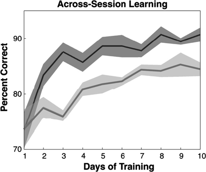
The second finding we wish to replicate is that of Seitz et al. (2006), who conducted experiments on human subjects to compare multisensory audio–visual learning with uni-sensory visual learning. He showed that using multisensory audio–visual training results in significantly faster learning than unisensory visual training, as depicted in Fig. 1. There has been a significant amount of research dedicated to understanding crossmodal or multisensory interactions, and their underlying mechanisms. The bulk of this research is being carried out in the fields of psychology, cognitive science and neuroscience. However, there is relatively little research devoted to developing computational models of multisensory interactions. We present a computational model that qualitatively reproduces the result shown in Fig. 1. We emphasize that our aim is to create a single computational model that can explain both these findings.
Fig. 1.
This figure, from Seitz et al. (2006) [Fig 3] shows the improvement in learning when multisensory learning (darker curve) is used instead of uni-sensory learning (lighter curve)
Though brain signals are time-varying, there are few computational models in the literature that directly address multisensory learning, while accommodating temporal aspects such as synchrony. The fundamental contribution of the current paper is to present an oscillatory neural network model that utilizes multisensory inputs to replicate semantic congruency effects and achieve faster learning. We present a principled, optimization-based approach to multisensory learning, based on sparse spatio-temporal encoding. The model derived from this approach produces experimental results that are consistent with observations in neuroscience and cognitive science, specifically those presented in Molholm et al. (2002) and Seitz et al. (2006). Such a development of computational models contributes to our understanding of fundamental brain processes. This paves the way for multiple advances including the building of machines with more human-like capabilities.
Background
Shams and Seitz (2008) propose that multisensory learning can be advantageous as objects in our world are simultaneously experienced through multiple senses. We expect that our brain has evolved to optimize this simultaneous processing, and this led Shams and Seitz (2008) to hypothesize that multisensory training protocols produce greater and more efficient learning. Due to the temporal nature of objects in the real world and their corresponding brain signals, we need to model multisensory training by paying attention to temporal synchrony in the presentation of different sensory streams originating from a single object.
Singer, Gray et al. (1989) discusses the potential role of synchrony in tagging the relatedness of events. Synchronization may serve as a computational substrate for encoding elementary Gestalt rules of grouping.
Van Rullen (2017) presents an interesting perspective regarding the state of current research in the field of perception science. Deep neural networks are very popular and have been applied widely (Schmidhuber 2015). However, there are many fundamental problems in perceptual processing such as color constancy, multisensory integration, and attention, which remain to be explored through deep networks. Furthermore there are several phenomena involving brain dynamics, such as oscillations, synchronization, and perceptual grouping which have not been explored by deep networks.
Yamashita et al. (2013) present a model that performs multisensory integration using a Bayesian approach. However, their model does not contain any temporal dynamics. Similarly, Rohde et al. (2016) and Fetsch et al. (2013) have developed statistical approaches to cue integration from multisensory signals, but do not address the aspect of temporal dynamics. van Atteveldt et al. (2014) review the recent neuroscientific findings in the area of multisensory integration. They emphasize the role of timing information such as oscillatory phase resetting in the processes involved in multisensory integration. However, they did not present specific computational models that embody this timing information.
Kopell et al. (2014) have proposed the concept of a “dynome”, which combines anatomical connectivity of the connectome with brain dynamics occurring over this anatomical substrate. They recognize the importance of temporal phenomena such as rhythms and its role in cognition.
In our current paper, we build a computational model using oscillatory elements. Networks using oscillatory elements have been investigated for nearly three decades, and form a viable platform to implement theories of synchronization (Grossberg and Somers 1991; Sompolinsky et al. 1990). However, controlling the dynamics of these oscillatory models has proven to be a challenge (Wang 1996). Hence, it is typical for oscillatory models to be tested on surrogated inputs, as for instance in the very recent papers Kazanovich and Borisyuk (2017) and Garagnani et al. (2017). Other efforts including Qu et al. (2014) and Balasubramaniam and Banu (2014) do not use specific sensory inputs, but rather investigate properties of the network connecting individual oscillators.
Jamone et al. (2016) review the concept of affordance arising from the psychology literature which is related to sensorimotor patterns created by a perceptual stimulus. Inherent in the notion of an affordance is the idea that action and perception are intertwined, and that action can influence perception. In this context, visuo-motor maps become important, and our framework could serve as a foundation for the integration of visual and motor representations.
Noda et al. (2014) present a computational model for multisensory integration. They use a deep auto-encoder to compress the data from multiple modalities, and a deep learning network to recognize higher-level multi-modal features.
The synchronization between multi-modal representations need not be confined to a single organism, but can extend across multiple organisms. Coco et al. (2016) review the role of sensory-motor matching mechanisms when two humans are involved in a joint co-operative task.
A body of research in the computational domain exists under the area of sensor fusion or data fusion, and has been reviewed by Khaleghi et al. (2013). The thrust of this work revolves mostly around understanding correlations and inconsistencies in data gathered from multiple channels with the goal of reducing uncertainty. Though there have been successful applications of this work in areas such as robotics, the focus is not on developing plausible models of brain function. Specifically, models of sensor fusion do not contain temporal dynamics such as synchronization, which are very relevant to understanding neural mechanisms that lead to perception. The computational model presented in the current paper explicitly deals with the phenomenon of neural synchronization, which contributes to a richer understanding of perceptual dynamics.
Methods
Our earlier research investigated a model based on the principle of sparse spatio-temporal encoding for processing sensory information (Rao et al. 2008; Rao and Cecchi 2010). The model was extended to two sensory pathways in Rao and Cecchi (2013).
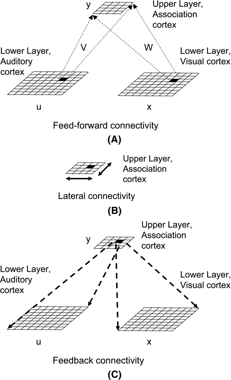
We review the model from Rao and Cecchi (2013) briefly. Figure 2, shows a two layer system with two input streams, a simulated audio and a simulated visual stream. Though these streams are termed ‘audio’ and ‘visual’, this is done for sake of concreteness, and our method should work with other combinations of sensing modalities such as tactile and visual for example.
Fig. 2.
A hierarchical organization of simulated cortical interactions. At the lower level, we have simulated visual and auditory cortices. These are mapped to a higher level area, termed the association cortex. a Depicts feed-forward connections, b depicts lateral connections and c depicts feedback connections
Let x denote units in the lower layer visual cortex, u denote units in the lower layer auditory cortex, and y denote units in the upper layer association cortex. We use a weight matrix to map the visual cortex to the association cortex. and a weight matrix to map the auditory cortex to the association cortex.
Computationally, each unit is modeled as an oscillator with an amplitude, frequency and phase of oscillation. If we assume that the units possess similar nominal frequencies, their behavior can be described by phasors of the form for the visual cortex, for the auditory cortex and for the association cortex. Here, and represent the amplitudes of units in the visual and auditory cortices and represents amplitudes of units in the association cortex. Similarly, and are the phases of the nth unit in the visual and auditory cortices, and represents phases of units in the association cortex. Note that frequency is equal to the rate of change of phase, so we do not explicitly represent frequency of oscillation in the following equations.
In our earlier work (Rao et al. 2008; Rao and Cecchi 2010), we formulated an objective function that achieves sparse spatio-temporal encoding of visual inputs. This work is based on a system of interconnected oscillators, and utilizes the amplitude and phases of the oscillators to achieve a stable network state where the upper layer units encode inputs conveyed at the lower layer. The detailed derivation of this model is outside the scope of this paper. Instead, we briefly review the essential dynamical update rules. Given a set of initial conditions, the system evolves dynamically as described by Eqs. 1–3.
| 1 |
| 2 |
| 3 |
| 4 |
Here, and are constants that are proportional to the desired sparsity of the values , as described in Rao et al. (2008). The parameter values are summarized in Table 1. The time step used to perform the updates in 1 and is ms. This is standard practice in the literature on Kuramoto oscillators, which serve as a model for synchronization phenomena (Acebrón et al. 2005).
Table 1.
| Parameter | Description | Value |
|---|---|---|
| Sparsity parameter controlling the influence of other units on a given unit | 0.25 | |
| Sparsity parameter controlling the influence of a unit on itself | 0.5 |
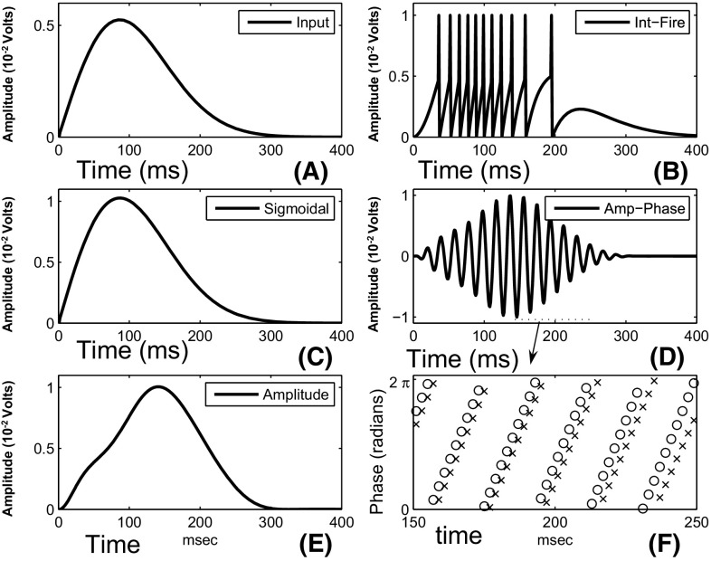
Figure 3 depicts the time-varying behavior of the oscillatory elements used in our model. This behavior is contrasted with other models of neural elements used in the literature.
Fig. 3.
The behavior of an oscillatory element contrasted with other types of elements. The x axis depicts time, and the y axis represents the amplitude of the neural units as a function of time. a Shows the input signal. b Depicts the output of an integrate-and-fire element. c Depicts the output of a typical sigmoidal neural element. d Depicts the real-valued output of the oscillatory element. e Depicts the amplitude of the oscillatory element. f Shows the phase of the oscillatory element in ‘o’ and the phase of the input element in ‘’. The oscillatory plot is created from Eq. 1
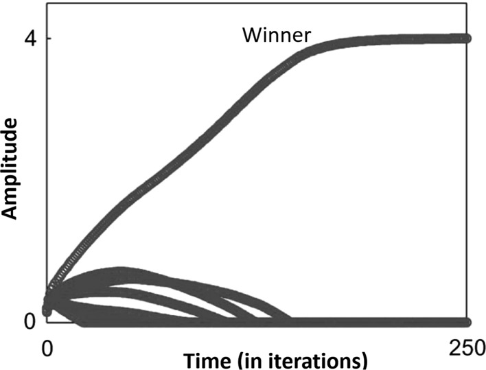
When Eqs. 1–3 are applied to the different units in the system, we observe that there are transients initially, such as in the amplitudes of the units as shown in Fig. 4. These settle down after approximately 200 iterations. The synaptic weights are updated after this settling period by using the equation:
| 5 |
A similar update is applied to .
| 6 |
Note that the phase of units in the system are a function of their natural frequency and the result of interactions with other units.
Fig. 4.
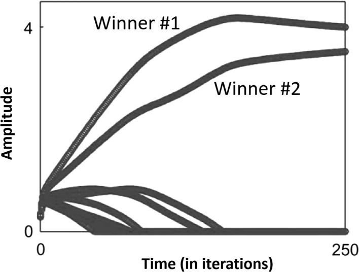
The evolution of amplitudes in the upper layer units is shown. In the steady state, a single winner emerges upon the presentation of a stimulus
Interpretation of network dynamics
Let us consider a single channel, say the visual channel, denote by lower layer units connected to upper layer units via weights . As discussed in Rao et al. (2008), the application of Eqs. 1–3 result in a winner-take-all dynamics amongst for a single input stimulus, where a single winner emerges amongst the upper layer units. This is illustrated in Fig. 4.
When two inputs are superimposed, two winners emerge, as shown in Figs. 4 and 5. To understand this, consider the following equation , where is the input to unit n. During steady-state, . Let the Mth input cause to attain its maximum value, , and hence . Here, the condition for stability implies , or equivalently . We can achieve this condition through proper alignment of the weight vectors after learning takes place.
Fig. 5.
This figure illustrates the evolution of amplitudes in the upper layer units when a superposition of two inputs is presented. In the steady state, two winners emerge, each representing one of the inputs
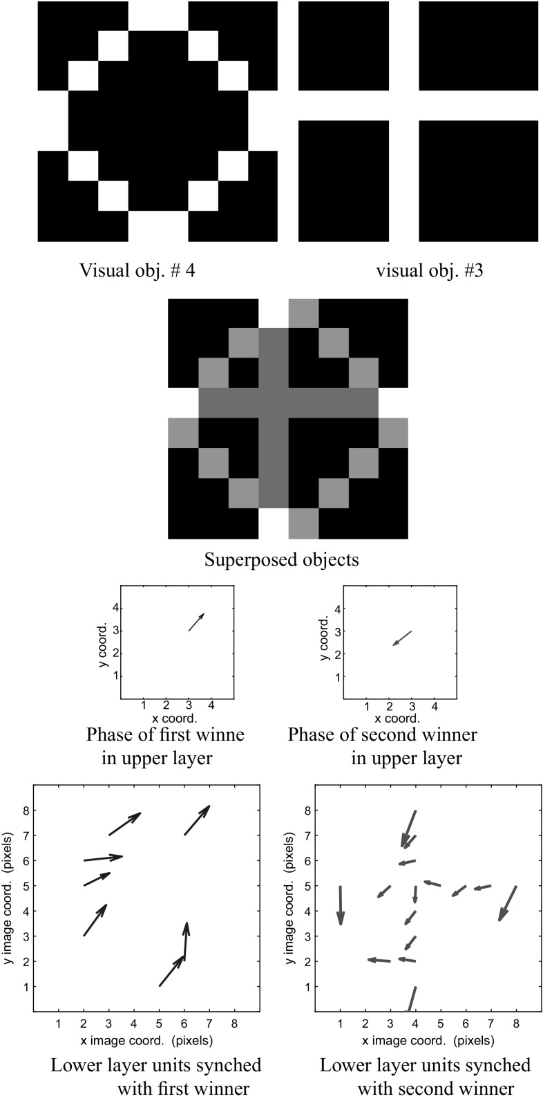
When two vectors are presented to the network after learning, we can conduct a similar analysis to show that a stable solution with two winners is possible when . We note that when two winners are present, their phases are in opposition, ie approximately radians apart, as shown later in Fig. 10.
Fig. 10.
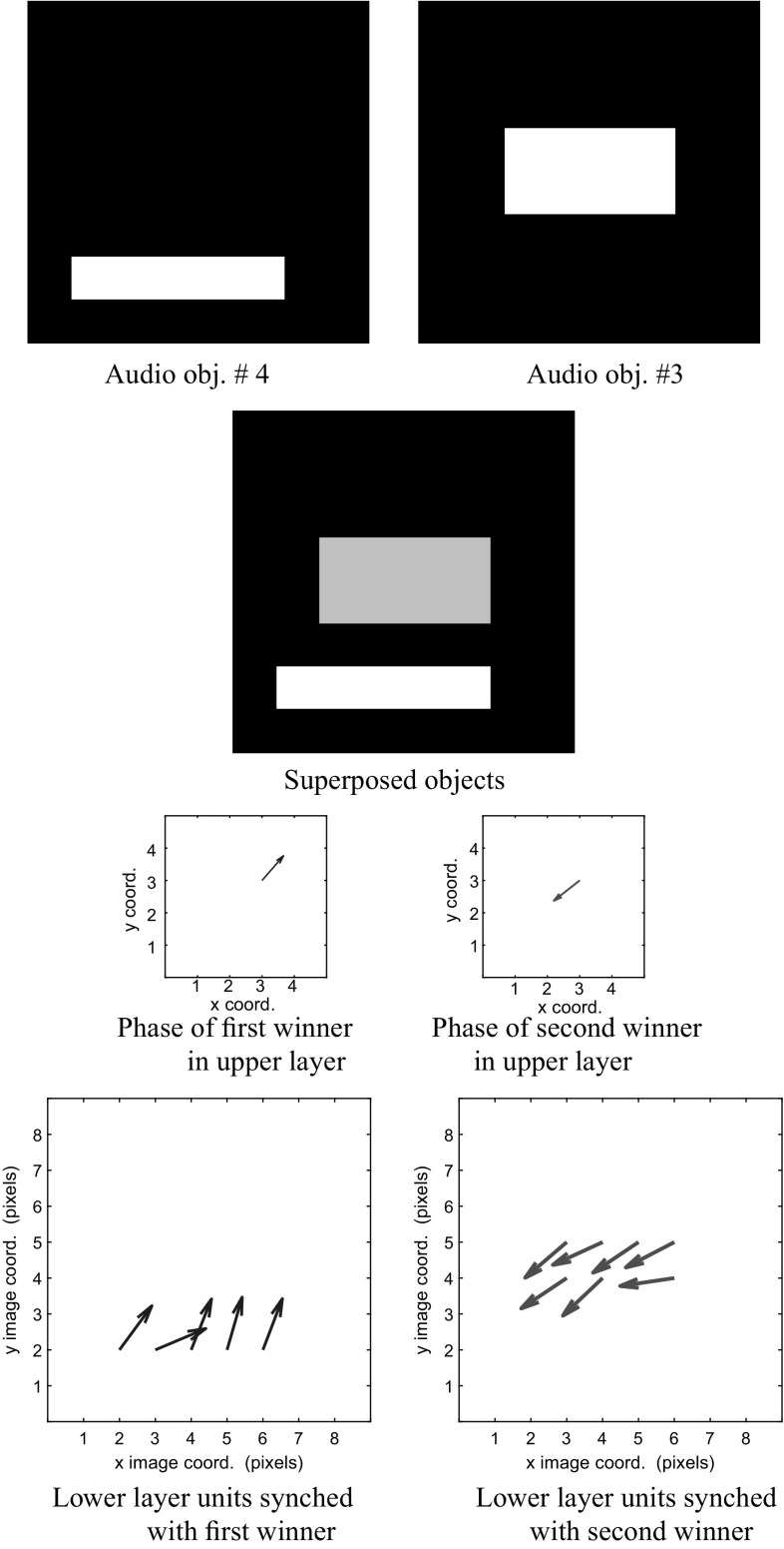
The auditory stream is depicted. We begin with the superposition of objects 4 and 3, and their corresponding visual maps. We normalize the grayscale image of the superposed objects before display. The phase of the first winner (in blue) corresponding to object 4 in the upper layer y is 0.588 radians. The phase of the second winner in y (in red) corresponding to object 3 is 3.767. We use a vector field to display the activity in the lower layers. The magnitude of a vector reflects the amount of activity in a unit, and its direction encodes the phase of the unit. (Color figure online)
Each of the Eqs. 1–3 can be understood in more detail as follows. In Eq. 1, the cosine term involving phase differences ensures that synchronized units, i.e. units with smaller phase differences have a stronger feed-forward effect on the amplitude. The excitatory feed-forward and feedback connections are such that units that are simultaneously active tend towards phase synchrony. The inhibitory connections tend to produce de-synchronization. At the same time, they also have a stronger suppressing effect on the amplitude of synchronized units, and correspondingly a weaker effect on the amplitude of de-synchronized units.
The equations for synaptic learning, Eqs. 5 and 6 consist of a simple extension of Hebbian learning, where simultaneous activity between two units is rewarded, with an additional cosine term that rewards the degree of synchronization between these two units. With this scheme, it is possible to admit two winners in the upper layer if their phases are radians apart, in which case the cosine term becomes zero.
Audio–visual stimulus presentation
Let us assume that the lower layer is initialized to contain pixel values of a 2-D visual image representing a visual stimulus and a 2-D audio image representing a simultaneously presented auditory stimulus. Since the audio and visual stimulus occur simultaneously in the real world, they are presented as a congruent pair. As noted earlier, we can combine any two sensory stimuli from different sensing modalities this way, which is consistent with an interpretation offered by Ghazanfar and Schroeder (2006). The upper layer, y is initialized to zero. and all phase values are randomized.
This pairing of the auditory and visual sensory information is consistent with the state-of-the-art in multisensory processing as reviewed by Murray et al. (2016). They stress that physical stimulus characteristics play a central role in influencing multisensory interactions at different abstraction levels, including neural, perceptual and behavioral levels. Key stimulus characteristics include spatial and temporal relationships between signals in different senses that emanate from physical objects.
The lower layer visual cortex consists of units, each of which receives a visual intensity value as input. Similarly, the lower layer auditory cortex consists of units receiving auditory intensity values as input.
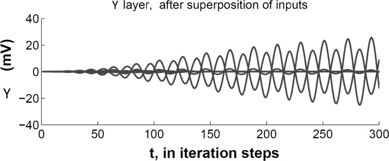
The upper layer y consists of 16 units. We utilize all-to-all connections between units x and y, and between u and y. Units in y are interconnected by all-to-all lateral connections, and there are all-to-all feedback connections from y to x and from y to u. When learning is completed, the units in the upper layer demonstrate a winner-take-all dynamics when an input is presented at the lower layer. In order to clarify the winner-take-all dynamics, we show the time-varying output of the winners in the upper layer in Fig. 6.
Fig. 6.
We plot the evolution of amplitudes in the and upper layer when two superposed inputs are presented. Each sinusoidal pattern shows the real-valued amplitude of a unit plotted on the vertical axis against time in iteration steps along the horizontal axis. There are two upper layer units that respond to the superposition. Note that these responses are out of phase with each other ( apart)
The representation in the time domain as shown in Fig. 6 can get cluttered for a large number of units, and it is difficult to convey spatial relationships in the same plot. Hence we use a phasor representation in subsequent plots, where the amplitude of the oscillation is represented by the length of a vector and the phase of the oscillation is represented by the angle of the vector. The time domain and phasor representations are equivalent.
In order to illustrate our model, we use an input set shown in Fig. 7 consisting of the following 4 simple visual objects: triangle, square, cross, and circle. These visual objects are associated with corresponding audio objects, as shown in Fig. 8. Thus, each real-world object generates a paired visual and auditory input pattern, known as a congruent pairing. The auditory objects are idealized representations of tonotopic maps consisting of frequencies arranged spatially (Formisano et al. 2003). As observed in the Background section, it is common in the literature on oscillatory neural networks to use such surrogated inputs, for instance as done recently by Kazanovich and Borisyuk (2017) and Garagnani et al. (2017).
Fig. 7.
A simulated representation of four objects in the visual cortex
Fig. 8.
A simulated representation of objects in the auditory cortex. The 2-d maps represent idealized tonotopic maps corresponding to the visual objects shown in Fig. 7
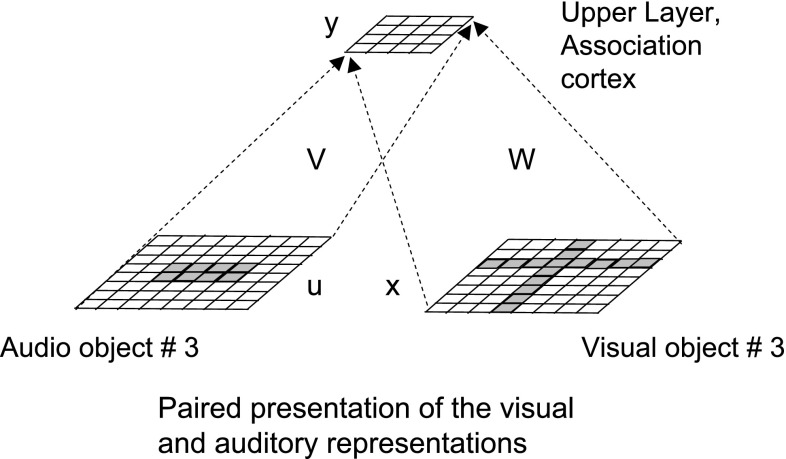
To create an object stimulation, we pair the auditory and visual representations, and present them jointly at the lower layer, as in Fig. 9.
Fig. 9.
We simulate an audio–visual object presentation by initializing the lower layers separately to the visual and auditory components of an object. This figure uses the visual and auditory representations of object #3 shown in Figs. 7 and 8 respectively
The network operates in two sequential stages, denoted by learning and performance. During the learning stage, a single randomly selected object is presented and the network activity settles down. The Hebbian learning rules from Eqs. 5 and 6 are applied, which represents unsupervised learning. This process is repeated over 1000 trials or presentations. The upper layer units in the association cortex, y, exhibit a winner-take-all behavior such that each input produces a unique winner.
During the performance phase, we present superpositions of two objects at a time. When two inputs are superposed and presented to the lower layer x, two winners emerge in the upper layer y. These units correspond to the two units with the two largest amplitudes. The phases of the winners in layer y are synchronized with the phases of units in the lower layers x and u that correspond to the two individual inputs. Hence, different units in the upper layer y can be simultaneously active while possessing phases that are maximally apart from each other, ideally radians apart. This facilitates an efficient separation of mixtures of objects based on their phase representations.
We quantify the network behavior through two measures, the separation accuracy and segmentation accuracy. The separation accuracy measures the ability of the network to correctly identify superposed inputs. Suppose unit i in the upper layer is the winner for an input , and unit j is the winner for input . If units i and j in the upper layer are also winners when the input presented is the mixture , then the separation is deemed to be correct. The separation accuracy is defined to be the ratio of the total number of correctly separated cases to the total number of cases.
The segmentation accuracy computes the degree to which the phases of unique distinct objects in the network are distinguishable from each other. We determine the fraction of the units of the lower layer that correspond to a given object and are within a given tolerance limit of the phase of the upper layer unit corresponding to the same object. This measure is termed the segmentation accuracy.
Results
Figures 10 and 11 show the system response when objects 4 and 3 are presented simultaneously. In Fig. 10 we show the result of superposing visual information arising from these two objects, while Fig. 11 shows the result of superposing auditory information.
Fig. 11.
The visual stream is examined. We show the superposition of objects 4 and 3 occurring in the auditory maps. In the upper layer y, the phase of the first winner (in blue), corresponding to object 4 is 0.588 radians. The phase of the second winner in y (in red), corresponding to object 3, is 3.767. The bottom row depicts the phases of the lower layer in the auditory maps. (Color figure online)
The third row of Fig. 10 shows that the two winners in the upper layer are approximately radians out of phase with each other. The phasors representing the winners are colored blue and red to help the reader compare them against the phasors in the lower layer. We can readily see that in the lower layer, phasors in blue are representative of visual object #4, and are synchronized with the blue phasor in the upper layer winner that denotes a higher-level representation of object #4. Similarly, the red-colored phasors in the lower and upper layers indicates a consistent representation of object #3 across these layers.
From Fig. 11 we observe that the correspondence between the phase information across hierarchical layers also holds true for the auditory representations of the same two objects. Thus, phase synchronization exists between the units in the lower layer for both auditory and visual maps corresponding to a given object and also the upper layer winner that represents the composite audio–visual object.
The mechanisms to attain the amplitudes and phases in Figs. 10 and 11 were reviewed in "Interpretation of network dynamics" section. Essentially, the amplitudes of the units in the upper layer are governed by a winner-take-all behavior, whereas the phases in the upper and lower layers co-evolve over each successive iteration. This co-evolution converges to a local minimum of an objective function representing a sparse spatio-temporal encoding of the input, as described in Rao et al. (2008) and Rao and Cecchi (2010). The net result is that a winner in the upper layer receives a phase that is close to the phases of the input layer units representing a single object. Furthermore, we showed in "Interpretation of network dynamics" section that two winners can exist in the upper layer provided their phases are approximately radians apart. Due to the phase synchronization of a winner in the upper layer with the input that it represents, it follows that there will be two sets of phases in the lower layer units, one for each winner, and that the phase separation between these sets is also approximately radians.
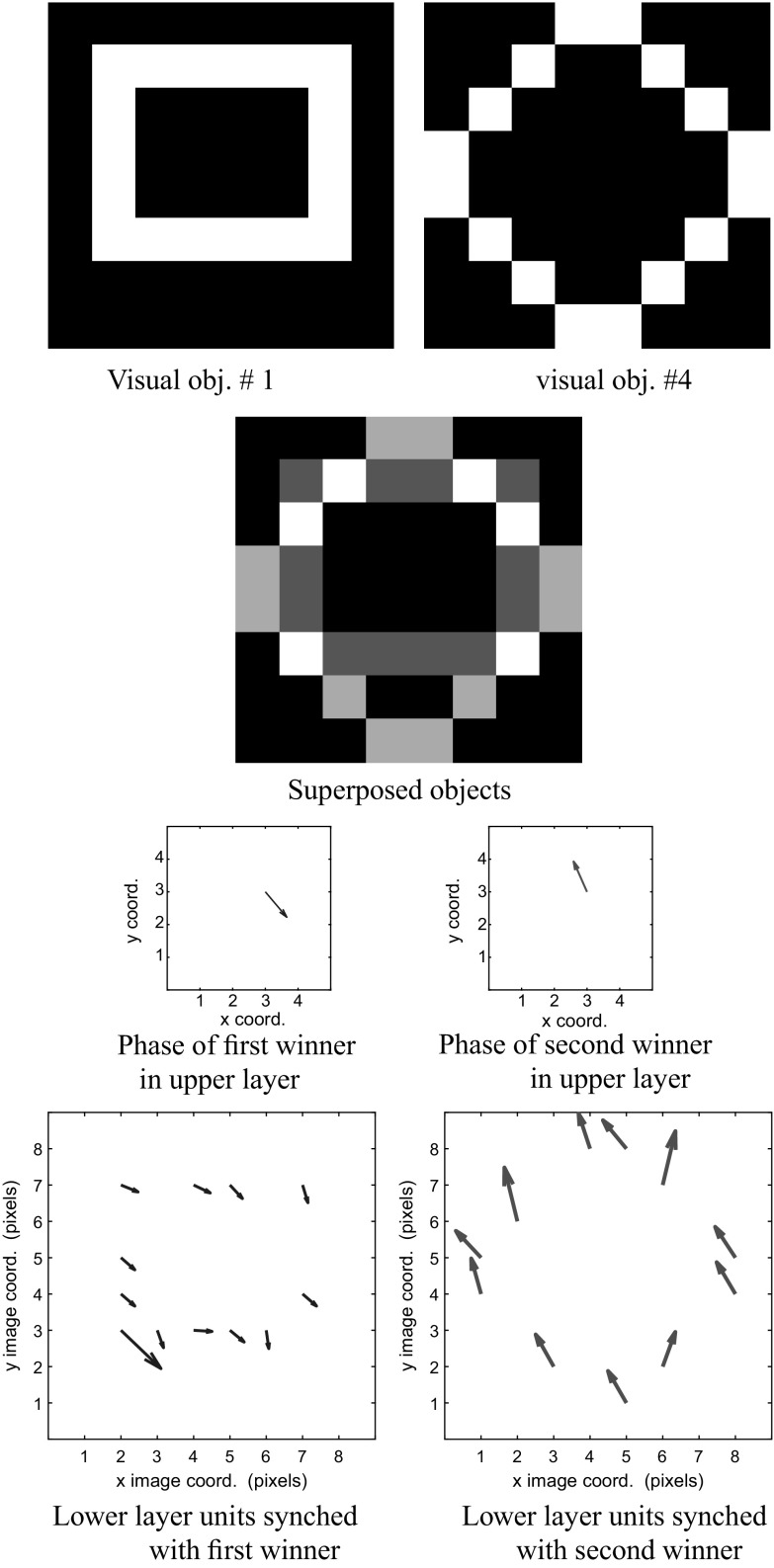
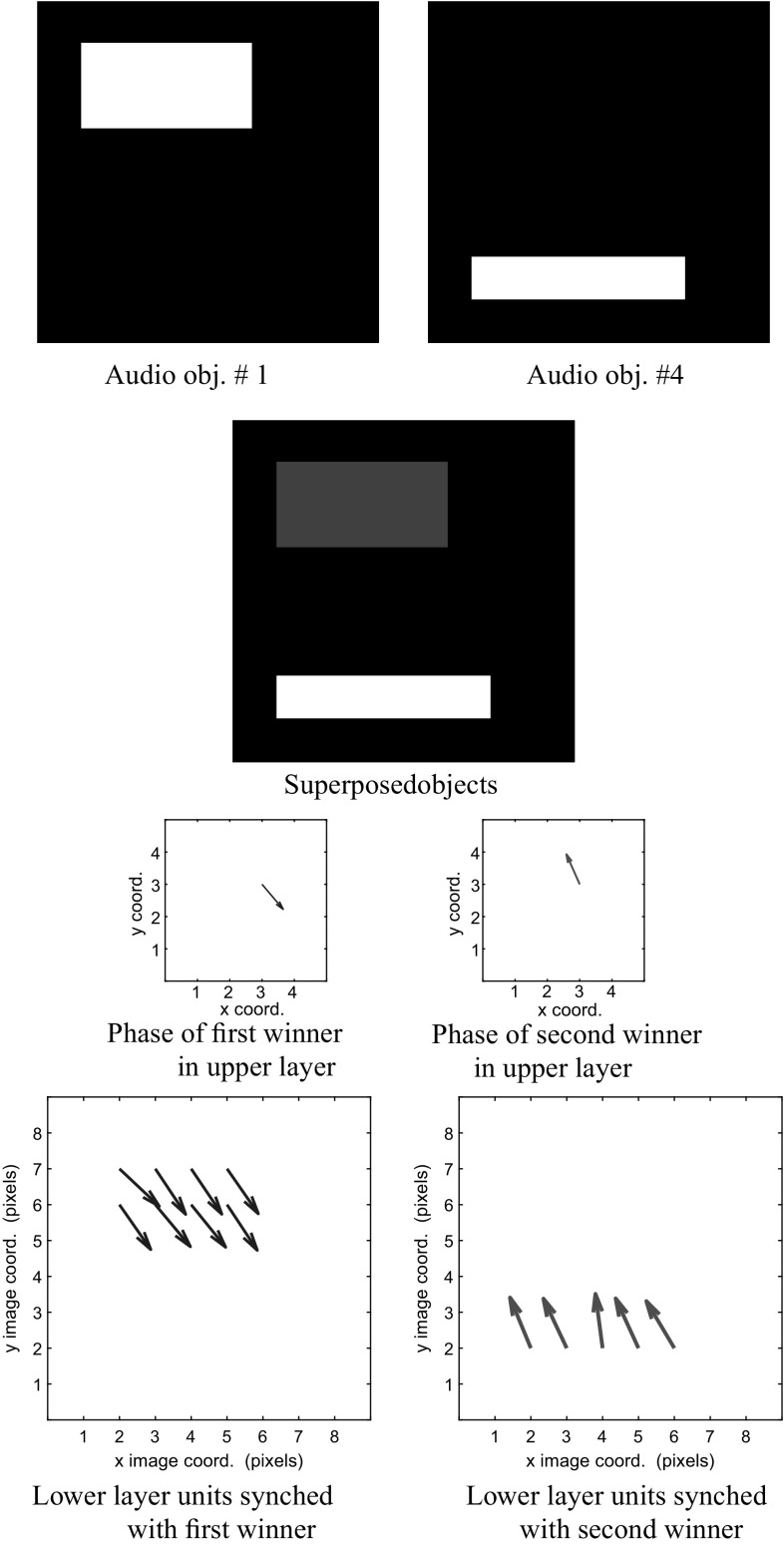
Figures 12 and 13 show a similar behavior for a mixture of objects 1 and 4. The network is able to separate both the audio and visual representations of these objects.
Fig. 12.
We examine the visual stream. Consider the superposition of objects 1 and 4, and their corresponding visual maps. We normalize the grayscale image of the superposed objects before display. The phase of the first winner corresponding to object 1 in the upper layer y (in blue) is 5.49 radians. The phase of the second winner in y (in red) corresponding to object 4)is 1.96 radians. We use a vector field to display the activity in the lower layers. The magnitude of the vector represents the amount of activity in the unit, and the direction of the vector encodes the phase of the unit. (Color figure online)
Fig. 13.
We examine the auditory stream by showing the superposition of objects 1 and 4, and the corresponding auditory maps. We normalize the grayscale image of the superposed objects before display. The phase of the first winner corresponding to object 1 in the upper layer y (in blue) is 5.49 radians. The phase of the second winner in y (in red) corresponding to object 4 is 1.96 radians. The phases of the lower layer in the auditory maps are displayed in the bottom row. (Color figure online)
We gathered statistics about the performance of the network via the following procedure. Let an epoch consist of:
A training phase, where the network learns its weights over 1000 presentations of the objects in random order and
A recall phase, which occurs after the weights are learned. During recall, we present combinations of a pair of objects and calculate the network response. We use the separation and segmentation accuracy to measure the system performance. We present 100 different pairwise combinations of objects, selected at random in order to compute the separation and segmentation accuracy.
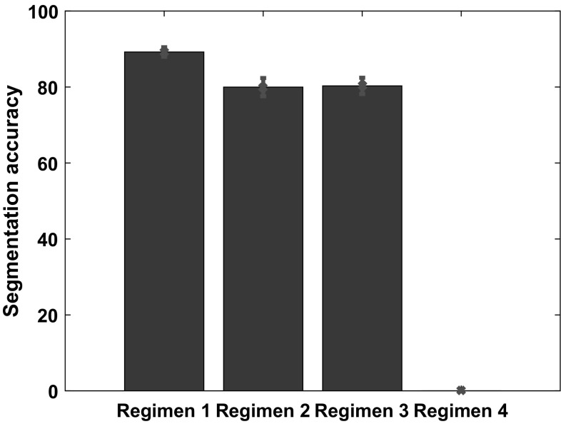
We obtained estimates of the separation and segmentation accuracy of the network over 60 epochs. We also varied the sensory pathways utilized according to the following four regimens.
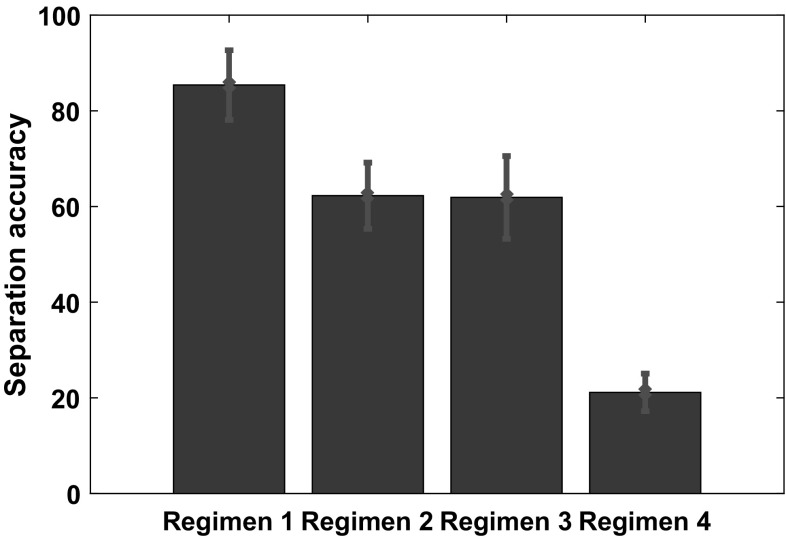
Regimen 1: Both the audio and visual pathways were used in training and recall.
Regimen 2: Both the audio and visual pathways were used in training but only the visual pathway was used during recall.
Regimen 3: Only the visual pathway was used for training and recall.
Regimen 4: Both the audio and visual pathways were used in training. However, during the recall phase, we modified the congruency between the audio and visual signals such that a visual object was paired with a different auditory stimulus than the one the network was trained with.
For each of the regimens, we calculated network performance measures averaged over 60 epochs. These values are analyzed as follows. First, we display the network performance measured by the separation accuracy in Fig. 14 and segmentation accuracy in Fig. 15. Second, we examine the statistical distributions formed by these performance statistics, e.g. a distribution of separation accuracies for each regimen. We utilize the two-sample Kolmogorov–Smirnov test to determine whether samples from two regimens arise from the same continuous distribution. This calculation is performed by using the function kstest2 in Matlab. The null hypothesis is that data in two vectors are from the same continuous distribution, in which case the function kstest2 returns a 0. If the null hypothesis is rejected at a 5% significance level, the function kstest2 returns a 1. Table 2 shows the results of comparing the distributions for separation accuracy under the above four regimens.
Fig. 14.
We compare the network performance across the following four regimens: Regimen 1: Both the audio and visual pathways were used in training and during recall. Regimen 2: Both the audio and visual pathways were used in training but only the visual pathway is used during recall. Regimen 3: Only the visual pathway is used during training and recall. Regimen 4: Both the audio and visual pathways are used in training. During the recall phase, we alter the congruency between the audio and visual signals. This means that a visual object is paired with a different auditory stimulus than the one the network was trained with. We plot the mean value of the separation accuracy for each regimen. The standard deviation is plotted in the form of red error bars
Fig. 15.
We compare the network performance across the different regimens as follows. The mean value of the segmentation accuracy is plotted along the y axis for each regimen. The standard deviation is plotted in the form of error bars, shown in red. Regimen 1: Both the audio and visual pathways were used in training as well as during recall. Regimen 2: Both the audio and visual pathways were used in training but only the visual pathway is used during recall. Regimen 3: Only the visual pathway is used during training and recall. We ignore Regimen 4, where non-congruent audio and visual signals are used during recall. This is because the separation accuracy is very low, and subsequently the results for the segmentation accuracy are not meaningful
Table 2.
Results of using the two-sample Kolmogorov–Smirnov test. This test determines the similarity of distributions of separation accuracies over multiple trials in each regimen
| Both visual and audio for training and recall | Train with audiovisual, recall with visual only | Train with visual and recall with visual | Train with audiovisual, recall with non- congruency | |
|---|---|---|---|---|
| Both visual and audio for training and recall | Dissimilar | Dissimilar | Dissimilar | |
| Train with audiovisual, recall with visual only | Similar | Dissimilar | ||
| Train with visual and recall with visual | Dissimilar | |||
| Train with audiovisual, recall with non-congruency |
Interestingly, the two-sample Kolmogorov–Smirnov test shows that all distributions of separation accuracy arising from the different regimens are dissimilar except in the following case. When the network is trained with audio–visual stimuli and only the visual pathway is used for recall, then the performance is statistically similar to the regimen where only the visual pathway is used for both training and recall. Figure 14 shows that superior network performance as measured by separation accuracy is achieved when audio–visual pathways are utilized during both the training and recall phases.
We investigate the strength and efficiency of multisensory learning through results depicted in Figs. 16, 17, 18 and 19. These results form the basis of a comparison of the computational results from our model against the results from human subjects obtained by Seitz et al. (2006) as shown in Fig. 1.
Fig. 16.
The variation of the separation accuracy as a function of the number of settling iterations. a–e show separate graphs for specific numbers of training samples used, ranging from 100 samples to 500 samples
Fig. 17.
The variation of the segmentation accuracy as a function of the number of settling iterations. a–e show separate graphs for specific numbers of training samples used, ranging from 100 samples to 500 samples
Fig. 18.
The variation of the separation accuracy as a function of the number of training samples. a–d show separate graphs for specific numbers of training iterations used, ranging from 50 to 200 iterations
Fig. 19.
The variation of the segmentation accuracy as a function of the number of training samples. a–d show separate graphs for specific numbers of training iterations used, ranging from 50 to 200 iterations
We use the metrics of separation accuracy and segmentation accuracy to measure how well our model can distinguish audio–visual objects.
The following variables are of interest in exploring the performance of our computational model: the number of settling iterations, the number of samples over which training is performed, the separation accuracy and the segmentation accuracy. We use the following values for the number of settling iterations: 50, 100, 150, 200. Recall that the oscillatory networks take time to settle, and learning takes place only after the number of settling iterations has been reached. We use the following values for the number of training samples: 5, 100, 200, 300, 400, 500. Each training sample consists of a presentation of a paired audio–visual stimulus when multisensory training is being investigated and an individual visual stimulus for the case of uni-sensory training. We visualize the relationships between these variables in a series of 2-D plots.
Figures 16 and 17 show that for a given number of training samples, both the separation accuracy and segmentation accuracy increase as the number of settling iterations increase. Furthermore, the multisensory audio–visual regimen shows greater accuracy than the uni-sensory visual-only regimen. The best performance is obtained for 500 training presentations or samples, and 200 settling iterations, though the improvements tend to flatten out. Similarly, Figs. 18 and 19 show that for a given number of settling iterations, both the separation accuracy and segmentation accuracy increase as the number of training samples increase. Furthermore, the multisensory audio–visual regimen shows greater accuracy than the uni-sensory visual-only regimen.
Discussion
The results shown in Figs. 10, 11, 12 and 13 are significant as there are very few instances in the literature of successful separation of superposed audio–visual inputs, such as the work of Darrell et al. (2000). Earlier efforts towards separation of superposed signals were mainly applied to auditory signals involved in the “cocktail party” effect (Haykin and Chen 2005).
As stated in the Introduction, our goal was to develop computational models to explain two findings in the field of cognitive science concerning the effect of congruency of audio–visual stimuli and the efficiency of multisensory learning. We examine our results towards achieving these goals in the following subsections.
Interpretation of network dynamics among the different regimes
As explained in "Interpretation of network dynamics" section, the amplitudes in the upper layer exhibit a winner-take-all behavior with a single winner for a single input, and two winners for a superposition of inputs. Due to simultaneous presentation of the audio and visual signals for a single coherent object, the co-occurrence of these signals is learnt and results in a single winner in the upper layer. Since the presentation of combined signals in the audio and visual channels causes faster activation of the upper layer units as opposed to the presentation of a single channel, a steady state is achieved more quickly, leading to faster learning. When superpositions of audio–visual signals are created for two objects, the corresponding winners for these objects are activated in the upper layer. The use of two channels provides more pathways to activate the higher layer units as compared to a single channel, which leads to more accurate learning. Hence the network performance with two channels used for training and recall will be superior to the case when only a single channel is used. Ultimately, the associations between the different features in the audio–visual channels that represent distinct objects is captured in the pattern of synaptic weights that are learnt.
If both the audio and visual channels are used for learning, and only one is used for recall, the learned synaptic weights are still representative of the original object features. This results in pathways that stimulate partial recall, which may still produce the correct answers, depending on the specific inputs presented to the system. Accordingly, the separation and segmentation accuracy produced by this regime is not as high as the first regime where both channels are used for learning and recall.
If the auditory and visual channels are made incongruent, then the previously learned object feature associations are no longer preserved, causing erroneous upper layer units to respond. This adversely affects the network performance, as shown in Fig. 14.
Congruent processing of audio–visual stimuli
We first examine our findings related to the congruent processing of audio–visual information. Figure 14 shows that superior network performance as measured by separation accuracy is achieved when audio–visual pathways are utilized during both training and recall. Hence we offer the interpretation that it is advantageous to use multiple sensory pathways for both training and recall.
Experiments using congruent and non-congruent stimuli in the psychology literature (Thelen et al. 2015) demonstrate that the presence of congruent visual and audio stimuli enhances perception and recall. Furthermore, Davis et al. (1999) show that auditory information is able enhance human performance in virtual environments. The implication of these results can be summed up in the phrase “use it or lose it”. If a multisensory pathway is available, it is best to use it, as it enhances performance.
There was a possibility that using audio–visual signals instead of only-visual signals for training would confer an advantage in the formation of percepts related to different objects, whereby information in both channels could potentially sculpt boundaries for these objects in a high-dimensional feature space. Then, these boundaries could help in object discrimination when only one pathway (e.g. only the visual pathway) is used for recall. Our results suggest that this is unlikely for the following reason. Let us compare Regimen 2 (where both the audio and visual pathways were used in training and only the visual pathway is used during recall) to Regimen 3 (only the visual pathway is used during training and recall), using Fig. 14 and Table 2. We observe that there is no statistically significant difference between these Regimens in terms of the separation accuracy.
A multisensory protocol achieves greater and more efficient learning
Our second goal was to computationally model the efficiency of learning using different combinations of multisensory stimuli. By comparing Figs. 16, 17, 18 and 19 with Fig. 1, we see that there is a qualitative similarity between our model and human performance. Specifically, we can see from Fig. 16a that the largest performance gain occurs at a settling iteration of 150, and at this value, the separation accuracy for audio–visual stimuli is about 80% higher than the separation accuracy for only-visual stimuli. Other performance gains may not be as high and this gain depends on the number of settling iterations used, and also the number of training samples.
We show through computational modeling that a multisensory protocol indeed achieves greater and more efficient learning. This achieves our objective to develop computational models consistent with findings related to multisensory integration in neuroscience and cognitive psychology.
In order to place our research in the right context, we briefly discuss the relevance of our results in relation to the existing literature on multisensory processing.
Multisensory processing in the brain
Driver and Noesselt (2008) review several studies that examine multisensory convergence zones in the brain. For instance, it is well known that neurons in the superior colliculus receive inputs from visual, auditory and somatosensory areas. multisensory neurons are also found in the superior temporal sulcus. Though there are higher level convergence zones, the interplay between multiple senses does not have to wait till these levels, and can occur earlier, even at the level of primary cortices (Driver and Noesselt 2008). There is evidence that multisensory interplay can occur at some traditional sensory-specific brain regions. multisensory convergence zones may also provide feedback to earlier sensory-specific cortical areas. Our current model uses such a scheme, where a multisensory convergence zone provides feedback to simulated visual and auditory cortices, as shown in Fig. 2.
Invasive electrophysiology techniques were used initially to investigate multisensory processing. These techniques are now being augmented by modalities such as fMRI and MEG (Amedi et al. 2005) which have led to the identification of areas involved in audio–visual integration including the superior temporal sulcus and superior temporal gyrus.
Thelen et al. (2015) investigated the phenomenon of incongruent pairings between auditory and visual stimuli. For example, a congruent pairing would consist of a picture of an owl being presented simultaneously with the sound it emits. Multisensory interactions affect memory formation and can subsequently influence unisensory processing. Memory representations can span multiple senses and can also be activated by input from a single sense. In the current paper, we did not model memory representation within each sense. This will require an extension of our model shown in Fig. 2, and is a topic for future research
Bahrick and Lickliter (2012) highlight the importance of temporal synchrony in the binding of multisensory stimulation. In the current paper, we utilize temporal synchrony in two ways. First, we use synchronized presentations of paired audio and visual stimuli during the training phase. Second, the individual neural units in the simulated auditory and visual cortices and association area are able to interact, leading to synchronized activity amongst these units. In our model, temporal synchrony facilitates the formation of multiple object representations that are concurrently active. Such precise computational models are lacking in the psychology literature in papers such as Bahrick and Lickliter (2012). It is desirable to devise computational models to explain experimental observations gathered from human subjects. The current paper strives to bridge this gap between observations in psychology and existing computational models.
Quak et al. (2015) examine the role of multisensory information in memorization and working memory. According to their view, working memory consists of unified cross-modal representations as opposed to individual unisensory representations. In our model, we use a unified cross-modal representation in the form of an association layer, as shown in Fig. 2. This could serve as the foundation of a working memory in a larger system, and a more thorough investigation is a proposed for future research.
According to Shams and Seitz (2008), multisensory training protocols produce greater and more efficient learning. Our experimental results, shown in Figs. 14 and 15 are in concurrence, as we demonstrate superior performance when multisensory information is combined rather than treated individually.
van Atteveldt et al. (2014) proposed different neuronal mechanisms that may be employed in multisensory integration, which includes oscillatory phase resetting. This is very relevant, as the our model specifically utilizes oscillatory networks and phases, and hence dovetails well with current neuroscientific theories.
Semantic congruency refers to the degree to which pairs of auditory and visual stimuli are matched (or mis-matched). There has been a resurgence of interest in semantic congruency, in the recent literature in multisensory integration (Spence 2011). Our simulations explored congruency effects by deliberately scrambling the correspondence between auditory and visual stimuli arising from a given object. Our results show that system performance degrades in the presence of incongruent stimuli and are in agreement with experimental findings in attention perception (Spence 2011).
Visual perception can be influenced by sound and touch. This effect can be seen at early stages of visual processing, including the primary visual cortex, as observed by Shams and Kim (2010). This indicates that a relevant computational model must allow the primary cortices to be influenced by crossmodal signals. We satisfy this requirement in our model, as we allow signals from the auditory stream to influence activity in a simulated primary visual cortex, and vice versa. This ability is enabled via feedback connections from a higher-level associative cortex to each of the primary cortices as shown in Fig. 2.
Bastiaansen and Hagoort (2006) review the EEG and MEG literature to show that neural synchrony is a plausible mechanism through which the brain integrates language specific features such as phonological, semantic and syntactic information that are represented in different brain areas. Garagnani et al. (2017) present a computational model that uses oscillatory elements and is sensitive to the difference between input stimuli consisting of valid word pattern and pseudo-word patterns. The valid word patterns are familiar, learned word patterns whereas pseudo-word patterns are created by randomly recombining sub-parts of valid word patterns. Their model is able to bind phonological patterns with semantic information through synchronization.
Murray et al. (2016) observe that the traditional view is that multisensory integration occurs at higher-level cortical association areas. This is the view that we have incorporated into our computational model. However, recent research is showing that sensory systems can affect each other even at early stages. For instance, Falchier et al. (2002) demonstrated anatomical connectivity from core areas of the auditory cortex and the polysensory area of the superior temporal plane (STP) to peripheral regions of area 17 in the primary visual cortex. We have not modeled this connectivity explicitly in our current work. The effect of direct auditory to visual cortex connectivity will be explored in a future research effort.
The model presented in our paper is consistent with the latest reviews of multisensory processing, as presented by Murray et al. (2016). Specifically, we have modeled crucial physical stimulus characteristics including spatial and temporal relationships such as the simultaneity of auditory-visual cues.
As Murray et al. (2016) have observed, surprisingly little work has focused on the interplay between lower and higher-level factors influencing multisensory processing. The research presented in our current paper offers a computational model of such an interplay. Though enormous strides have been made by researchers in deep learning, the rich temporal dynamics observed in real brains has not received commensurate attention as observed by Van Rullen (2017). We expect that the research in the current paper can be extended to deep neural networks, which should be an interesting area for future research.
Socher et al. (2011) use the same deep neural network to parse visual scenes and natural language words. Their algorithm utilizes the recursive structure that is common to both visual scenes and natural language constructs. Though oscillatory models have been developed for visual (Rao et al. 2008) and audio processing (Wang and Brown 1999), their applications to language processing such as lexical and semantic analysis appear to be less explored. Research on this topic utilizing models of individual neural interactions has begun to appear recently (Garagnani et al. 2017). Much of the earlier work in understanding oscillatory behavior during language processing was at a higher level, involving EEG and fMRI recordings (Bastiaansen and Hagoort 2006), which do not analyze the explicit behavior of individual neurons.
A multimodal representation is useful in many contexts such as jointly searching for visual and textual information in a corpus. Feng and Lapata (2010) have developed a method that creates a bag-of-words representation for textual information, and derives image features to create a separate bag-of-words for visual information, called “visiterms” (for visual terms). Such combined textual and visual information is commonly found in news articles containing pictures. A topic model is then learned which concatenates the textual and visual bag-of-words. Though our technique does not compute a bag-of-words, the association between paired audio and visual signals arising from unique objects is represented as synaptic weights in our model.
The work of Mudrik et al. (2010) shows that semantic incongruency can occur through mismatches between two senses and also through inconsistent information within a single sensory modality. For instance, we do not expect to see a visual scene where a woman puts a chess board into an oven instead of a pie. Mudrik et al. (2010) measured the ERP through EEG recordings and showed that scenes that contain consistent information are interpreted faster and more accurately than scenes that contain inconsistent information. This forms the basis of an interesting experiment to conduct with the computational model we have provided, and is a topic for future research.
Though the network dynamics we presented in Eqs. 1–3 are independent of the number of units in the different layers of the network, we did not verify this experimentally. As a future research topic, we will experimentally examine the behavior of the network as the number of units is increased.
The connectivity shown in Fig. 2 does not show direct connections between the simulated primary visual and auditory cortices. There is evidence in the literature to support the existence of this type of connectivity. Bavelier and Neville (2002) review studies that use tracers to determine such connectivity, which is thought to affect peripheral vision. It would be interesting in future research to extend the model in Fig. 2 to include direct connections between the u and x layers representing simulated auditory and visual cortices. The specific connectivity can be designed to simulate the stimulation of peripheral vision.
Wang et al. (2011) demonstrate that the transmission delay between two units in a network can affect the emergence of synchronous oscillations in scale-free networks. Guo et al. (2012) have also investigated the role of fast spiking inhibitory interneurons in facilitating synchrony. They varied the synaptic delays and also the reliability of information transmitted across the synapse. In our model, we have not taken variable transmission delays into account. Future research needs to be performed to account for variable delays depending on the the length of anatomical connections between units in the different layers. This will improve the anatomical fidelity of our proposed model.
Yilmaz et al. (2013) show that stochastic resonance, involving suitably small levels of noise can improve network performance by amplifying weak signals. They also investigated the role of different synapse types including chemical and electrical. In contrast, our current model utilizes a single synapse type, and we do not model noise explicitly.
Guo et al. (2017) consider the behavior of a neural system that responds to superposed signals of different frequencies. In the current paper, we consider only a narrow range of frequencies. In the future, it would be interesting to extend the modeling techniques of the current paper to multiple frequency bands.
Relevance to other disciplines
Research in multisensory learning and perception can influence many other fields including education. There is growing interest in encouraging students to use better strategies to improve their learning, and ultimately their performance. Recent research highlights the importance of note-taking (Lee et al. 2013). Studies have shown Kiewra (2002) that handwritten notes are effective in improving student performance. One possible explanation for this phenomenon is that handwriting requires visuo-haptic and visuo-motor skills and exercises several brain circuits including the basal ganglia and cerebellum (Hikosaka et al. 2002). Though the computational results in the current paper were aimed at demonstrating audio–visual sensory integration, our approach is quite general, and could also apply to a combination of sensory modalities such as visual and haptic. Our results show that we can expect greater and more efficient learning when multiple sensory modalities are combined. Further computational modeling should help determine the expected performance improvements as shown in Figs. 16, 17, 18 and 19. For instance, our model predicts that when two sensory modalities are combined, there is an improvement of about 33% as measured by the separation accuracy.
Conclusion
The computational modeling of brain function, including simulation techniques has emerged as a powerful scientific tool over the past decade. However, current computational models are not able to satisfactorily explain recent findings regarding multisensory learning in the fields of neuroscience and cognitive science. A major challenge is to build a single model that explains multiple observed neural and cognitive phenomena such as temporal synchronization, binding and multisensory integration. We addressed this challenge by presenting a computational model for multisensory integration based on a theory of sparse spatio-temporal encoding of input stimuli. We apply our model to two input streams consisting of simulated auditory and visual information.
Through this computational model, we mirror the observations of researchers in psychology and neuroscience that multisensory integration produces greater and more efficient learning. By varying the learning protocol, system dynamics and duration of learning, we demonstrate that multisensory learning improves the system performance by up to 80% for object separation tasks. Furthermore, we show that the use of non-congruent stimuli results in significantly worse recall performance of the network. When a sensory input channel becomes disabled, we show that the network performance also degrades, but the degradation is less than that experienced when non-congruent stimuli are presented.
Our computational model produces simulation results that are consistent with observations regarding multisensory learning in neuroscience and cognitive science. The theoretical and experimental foundation we have provided can be generalized to more complex network architectures and the combination of additional sensory channels. This research contributes to our understanding of fundamental brain processes, and could facilitate multiple advances including the building of machines with more human-like capabilities.
Acknowledgements
The author greatly appreciates helpful comments from the reviewers, which improved this manuscript.
References
- Acebrón JA, Bonilla LL, Vicente CJP, Ritort F, Spigler R. The kuramoto model: a simple paradigm for synchronization phenomena. Rev Mod Phys. 2005;77(1):137. doi: 10.1103/RevModPhys.77.137. [DOI] [Google Scholar]
- Amedi A, von Kriegstein K, van Atteveldt NM, Beauchamp M, Naumer MJ. Functional imaging of human crossmodal identification and object recognition. Exp Brain Res. 2005;166(3–4):559–571. doi: 10.1007/s00221-005-2396-5. [DOI] [PubMed] [Google Scholar]
- Bahrick LE, Lickliter R. The role of intersensory redundancy in early perceptual, cognitive, and social development. In: Bremner A, Lewkowicz DJ, Spence C, editors. Multisensory development. Oxford: Oxford University Press; 2012. pp. 183–205. [Google Scholar]
- Balasubramaniam P, Banu LJ. Synchronization criteria of discrete-time complex networks with time-varying delays and parameter uncertainties. Cognit Neurodyn. 2014;8(3):199–215. doi: 10.1007/s11571-013-9272-y. [DOI] [PMC free article] [PubMed] [Google Scholar]
- Bastiaansen M, Hagoort P. Oscillatory neuronal dynamics during language comprehension. Prog Brain Res. 2006;159:179–196. doi: 10.1016/S0079-6123(06)59012-0. [DOI] [PubMed] [Google Scholar]
- Bavelier D, Neville HJ. Cross-modal plasticity: Where and how? Nat Rev Neurosci. 2002;3(6):443. doi: 10.1038/nrn848. [DOI] [PubMed] [Google Scholar]
- Coco M, Badino L, Cipresso P, Chirico A, Ferrari E, Riva G, Gaggioli A, D’Ausilio A. Multilevel behavioral synchronisation in a joint tower-building task. IEEE Trans Cognit Dev Syst. 2016;99:1–1. [Google Scholar]
- Darrell T, Fisher Iii JW, Viola P (2000) Audio-visual segmentation and the cocktail party effect. In: Advances in multimodal interfaces ICMI 2000. Springer, pp 32–40
- Davis ET, Scott K, Pair J, Hodges LF, Oliverio J (1999) Can audio enhance visual perception and performance in a virtual environment? In: Proceedings of the human factors and ergonomics society annual meeting, vol. 43, no. 22. SAGE Publications, pp 1197–1201
- Driver J, Noesselt T. Multisensory interplay reveals crossmodal influences on sensory-specificbrain regions, neural responses, and judgments. Neuron. 2008;57(1):11–23. doi: 10.1016/j.neuron.2007.12.013. [DOI] [PMC free article] [PubMed] [Google Scholar]
- Falchier A, Clavagnier S, Barone P, Kennedy H. Anatomical evidence of multimodal integration in primate striate cortex. J Neurosci. 2002;22(13):5749–5759. doi: 10.1523/JNEUROSCI.22-13-05749.2002. [DOI] [PMC free article] [PubMed] [Google Scholar]
- Feng Y, Lapata M (2010) Visual information in semantic representation. In: Human language technologies: the, (2010) annual conference of the north American chapter of the association for computational linguistics. Association for Computational Linguistics, pp 91–99
- Fetsch CR, DeAngelis GC, Angelaki DE. Bridging the gap between theories of sensory cue integration and the physiology of multisensory neurons. Nat Rev Neurosci. 2013;14(6):429–442. doi: 10.1038/nrn3503. [DOI] [PMC free article] [PubMed] [Google Scholar]
- Formisano E, Kim D, Di Salle F, van de Moortele P, Ugurbil K, Goebel R. Mirror-symmetric tonotopic maps in human primary auditory cortex. Neuron. 2003;40(4):859–869. doi: 10.1016/S0896-6273(03)00669-X. [DOI] [PubMed] [Google Scholar]
- Garagnani M, Lucchese G, Tomasello R, Wennekers T, Pulvermüller F. A spiking neurocomputational model of high-frequency oscillatory brain responses to words and pseudowords. Front Comput Neurosci. 2017 doi: 10.3389/fncom.2016.00145. [DOI] [PMC free article] [PubMed] [Google Scholar]
- Gershman SJ, Horvitz EJ, Tenenbaum JB. Computational rationality: a converging paradigm for intelligence in brains, minds, and machines. Science. 2015;349(6245):273–278. doi: 10.1126/science.aac6076. [DOI] [PubMed] [Google Scholar]
- Ghazanfar AA, Schroeder CE. Is neocortex essentially multisensory? Trends Cognit Sci. 2006;10(6):278–285. doi: 10.1016/j.tics.2006.04.008. [DOI] [PubMed] [Google Scholar]
- Gray C, König P, Engel A, Singer W. Oscillatory responses in cat visual cortex exhibit inter-columnar synchronization which reflects global stimulus properties. Nature. 1989;338(6213):334–337. doi: 10.1038/338334a0. [DOI] [PubMed] [Google Scholar]
- Grossberg S, Somers D. Synchronized oscillations during cooperative feature linking in a cortical model of visual perception. Neural Netw. 1991;4(4):453–466. doi: 10.1016/0893-6080(91)90041-3. [DOI] [Google Scholar]
- Guo D, Wang Q, Perc M. Complex synchronous behavior in interneuronal networks with delayed inhibitory and fast electrical synapses. Phys Rev E. 2012;85(6):061905. doi: 10.1103/PhysRevE.85.061905. [DOI] [PubMed] [Google Scholar]
- Guo D, Perc M, Zhang Y, Xu P, Yao D. Frequency-difference-dependent stochastic resonance in neural systems. Phys Rev E. 2017;96(2):022415. doi: 10.1103/PhysRevE.96.022415. [DOI] [PubMed] [Google Scholar]
- Haykin S, Chen Z. The cocktail party problem. Neural Comput. 2005;17(9):1875–1902. doi: 10.1162/0899766054322964. [DOI] [PubMed] [Google Scholar]
- Hikosaka O, Nakamura K, Sakai K, Nakahara H. Central mechanisms of motor skill learning. Curr Opin Neurobiol. 2002;12(2):217–222. doi: 10.1016/S0959-4388(02)00307-0. [DOI] [PubMed] [Google Scholar]
- Jamone L, Ugur E, Cangelosi A, Fadiga L, Bernardino A, Piater J, Santos-Victor J. Affordances in psychology, neuroscience and robotics: a survey. IEEE Trans Cognit Dev Syst. 2016;99:1–1. [Google Scholar]
- Kazanovich Y, Borisyuk R. Reaction times in visual search can be explained by a simple model of neural synchronization. Neural Netw. 2017;87:1–7. doi: 10.1016/j.neunet.2016.12.003. [DOI] [PubMed] [Google Scholar]
- Khaleghi B, Khamis A, Karray FO, Razavi SN. Multisensor data fusion: a review of the state-of-the-art. Inf Fusion. 2013;14(1):28–44. doi: 10.1016/j.inffus.2011.08.001. [DOI] [Google Scholar]
- Kiewra KA. How classroom teachers can help students learn and teach them how to learn. Theory Pract. 2002;41(2):71–80. doi: 10.1207/s15430421tip4102_3. [DOI] [Google Scholar]
- Kopell NJ, Gritton HJ, Whittington MA, Kramer MA. Beyond the connectome: the dynome. Neuron. 2014;83(6):1319–1328. doi: 10.1016/j.neuron.2014.08.016. [DOI] [PMC free article] [PubMed] [Google Scholar]
- Lee P-L, Wang C-L, Hamman D, Hsiao C-H, Huang C-H. Notetaking instruction enhances students’ science learning. Child Dev Res. 2013 doi: 10.1155/2013/831591. [DOI] [Google Scholar]
- Molholm S, Ritter W, Murray MM, Javitt DC, Schroeder CE, Foxe JJ. Multisensory auditory-visual interactions during early sensory processing in humans: a high-density electrical mapping study. Cognit Brain Res. 2002;14(1):115–128. doi: 10.1016/S0926-6410(02)00066-6. [DOI] [PubMed] [Google Scholar]
- Mudrik L, Lamy D, Deouell LY. Erp evidence for context congruity effects during simultaneous object-scene processing. Neuropsychologia. 2010;48(2):507–517. doi: 10.1016/j.neuropsychologia.2009.10.011. [DOI] [PubMed] [Google Scholar]
- Murray MM, Thelen A, Thut G, Romei V, Martuzzi R, Matusz PJ. The multisensory function of the human primary visual cortex. Neuropsychologia. 2016;83:161–169. doi: 10.1016/j.neuropsychologia.2015.08.011. [DOI] [PubMed] [Google Scholar]
- Noda K, Arie H, Suga Y, Ogata T. Multimodal integration learning of robot behavior using deep neural networks. Robot Auton Syst. 2014;62(6):721–736. doi: 10.1016/j.robot.2014.03.003. [DOI] [Google Scholar]
- Qu J, Wang R, Yan C, Du Y. Oscillations and synchrony in a cortical neural network. Cognit Neurodyn. 2014;8(2):157–166. doi: 10.1007/s11571-013-9268-7. [DOI] [PMC free article] [PubMed] [Google Scholar]
- Quak M, London RE, Talsma D. A multisensory perspective of working memory. Front Hum Neurosci. 2015 doi: 10.3389/fnhum.2015.00197. [DOI] [PMC free article] [PubMed] [Google Scholar]
- Rao A, Cecchi G. An objective function utilizing complex sparsity for efficient segmentation. Int J Intell Comput Cybern. 2010;3(2):173–206. doi: 10.1108/17563781011049160. [DOI] [Google Scholar]
- Rao AR, Cecchi G (2013) Multi-sensory integration using sparse spatio-temporal encoding. In: Neural networks (IJCNN), The 2013 international joint conference on. IEEE, pp 1–8
- Rao AR, Cecchi GA, Peck CC, Kozloski JR. Unsupervised segmentation with dynamical units. IEEE Trans Neural Netw. 2008;19(1):168–182. doi: 10.1109/TNN.2007.905852. [DOI] [PubMed] [Google Scholar]
- Rohde M, van Dam LC, Ernst MO. Statistically optimal multisensory cue integration: a practical tutorial. Multisens Res. 2016;29(4–5):279–317. doi: 10.1163/22134808-00002510. [DOI] [PubMed] [Google Scholar]
- Schmidhuber J. Deep learning in neural networks: an overview. Neural Netw. 2015;61:85–117. doi: 10.1016/j.neunet.2014.09.003. [DOI] [PubMed] [Google Scholar]
- Seitz AR, Kim R, Shams L. Sound facilitates visual learning. Curr Biol. 2006;16(14):1422–1427. doi: 10.1016/j.cub.2006.05.048. [DOI] [PubMed] [Google Scholar]
- Shams L, Kim R. Crossmodal influences on visual perception. Phys Life Rev. 2010;7(3):269–284. doi: 10.1016/j.plrev.2010.04.006. [DOI] [PubMed] [Google Scholar]
- Shams L, Seitz AR. Benefits of multisensory learning. Trends Cognit Sci. 2008;12(11):411–417. doi: 10.1016/j.tics.2008.07.006. [DOI] [PubMed] [Google Scholar]
- Socher R, Lin CC, Manning C, Ng AY, (2011) Parsing natural scenes and natural language with recursive neural networks. In: Proceedings of the 28th international conference on machine learning (ICML-11), pp 129–136
- Sompolinsky H, Golomb D, Kleinfeld D. Global processing of visual stimuli in a neural network of coupled oscillators. Proc Natl Acad Sci. 1990;87(18):7200–7204. doi: 10.1073/pnas.87.18.7200. [DOI] [PMC free article] [PubMed] [Google Scholar]
- Spence C. Crossmodal correspondences: a tutorial review. Atten Percept Psychophys. 2011;73(4):971–995. doi: 10.3758/s13414-010-0073-7. [DOI] [PubMed] [Google Scholar]
- Thelen A, Talsma D, Murray MM. Single-trial multisensory memories affect later auditory and visual object discrimination. Cognition. 2015;138:148–160. doi: 10.1016/j.cognition.2015.02.003. [DOI] [PubMed] [Google Scholar]
- van Atteveldt N, Murray MM, Thut G, Schroeder CE. Multisensory integration: flexible use of general operations. Neuron. 2014;81(6):1240–1253. doi: 10.1016/j.neuron.2014.02.044. [DOI] [PMC free article] [PubMed] [Google Scholar]
- van der Velde F, de Kamps M. Synchrony in the eye of the beholder: an analysis of the role of neural synchronization in cognitive processes. Brain Mind. 2002;3(3):291–312. doi: 10.1023/A:1022908120929. [DOI] [Google Scholar]
- Van Rullen R (2017) Perception science in the age of deep neural networks, Frontiers in Psychology, vol. 8, p. 142, [Online]. Available: http://journal.frontiersin.org/article/10.3389/fpsyg.2017.00142 [DOI] [PMC free article] [PubMed]
- Von der Malsburg C. The what and why of binding: the modelers perspective. Neuron. 1999;24(1):95–104. doi: 10.1016/S0896-6273(00)80825-9. [DOI] [PubMed] [Google Scholar]
- Wang L. Oscillatory and chaotic dynamics in neural networks under varying operating conditions. IEEE Trans Neural Netw. 1996;7(6):1382–1388. doi: 10.1109/72.548166. [DOI] [PubMed] [Google Scholar]
- Wang DL, Brown GJ. Separation of speech from interfering sounds based on oscillatory correlation. IEEE Trans Neural Netw. 1999;10(3):684–697. doi: 10.1109/72.761727. [DOI] [PubMed] [Google Scholar]
- Wang Q, Chen G, Perc M. Synchronous bursts on scale-free neuronal networks with attractive and repulsive coupling. PLoS ONE. 2011;6(1):e15851. doi: 10.1371/journal.pone.0015851. [DOI] [PMC free article] [PubMed] [Google Scholar]
- Yamashita I, Katahira K, Igarashi Y, Okanoya K, Okada M. Recurrent network for multisensory integration-identification of common sources of audiovisual stimuli. Front Comput Neurosci. 2013 doi: 10.3389/fncom.2013.00101. [DOI] [PMC free article] [PubMed] [Google Scholar]
- Yilmaz E, Uzuntarla M, Ozer M, Perc M. Stochastic resonance in hybrid scale-free neuronal networks. Physica A Stat Mech Its Appl. 2013;392(22):5735–5741. doi: 10.1016/j.physa.2013.07.011. [DOI] [Google Scholar]


