CAMS-RS: Clustering Algorithm for Large-Scale Mass Spectrometry Data Using Restricted Search Space and Intelligent Random Sampling

Abstract

High-throughput mass spectrometers can produce massive amounts of redundant data at an astonishing rate with many of them having poor signal-to-noise (S/N) ratio. These low S/N ratio spectra may not get interpreted using conventional spectra-to-database matching techniques. In this paper, we present an efficient algorithm, CAMS-RS (Clustering Algorithm for Mass Spectra using Restricted Space and Sampling) for clustering of raw mass spectrometry data. CAMS-RS utilizes a novel metric (called F-set) that exploits the temporal and spatial patterns to accurately assess similarity between two given spectra. The F-set similarity metric is independent of the retention time and allows clustering of mass spectrometry data from independent LC-MS/MS runs. A novel restricted search space strategy is devised to limit the comparisons of the number of spectra. An intelligent sampling method is executed on individual bins that allow merging of the results to make the final clusters. Our experiments, using experimentally generated data sets, show that the proposed algorithm is able to cluster spectra with high accuracy and is helpful in interpreting low S/N ratio spectra. The CAMS-RS algorithm is highly scalable with increasing number of spectra and our implementation allows clustering of up to a million spectra within minutes.

1. Introduction

MASS spectrometry is an immensely important tool in modern proteomics research used for protein identification and quantification [12]. Mass spectrometers measure the mass-to-charge ratio (m/z) of ionized molecules [31]. In the case of a typical LC-MS/MS proteomics experiment, ionized peptides are introduced into a mass spectrometer at the ion source in the form of liquid solutions, then desolvated and transferred into the gas phase as ions. Large-scale proteomics studies using mass spectrometry have useful applications in biological research such as studying the regulation of cellular processes [19], cancer molecular therapeutics [18] and others [13], [17]. The data generated from these machines is stochastic in nature and complex algorithms are required for post-processing of the raw data, e.g., phosphopeptide filtering [14], false positive rate estimation [4], quantification of proteins from large data sets [13], and phosphorylation site assignments [24], [26]. Other advanced methods include techniques to discriminate between different ions [32], estimating the probabilities of random match between an experimental-theoretical spectral pair [11], and identification of specific protein interactions using MS data [20]. As more high-throughput mass spectrometers are introduced, more efficient and novel computational tools are required to deal with these large data sets. Mass spectrometry often generates tens of thousands of spectra in a single run that need to be analyzed. The usual computational analysis route taken by most scientists is to take the raw data and search the spectra against a protein database of a known species (spectra-to-database matching). Search tools such as Sequest [7], Mascot [8], and X!tandem do a brute force execution of spectral matching and try to deduce the peptide corresponding to a given spectra. These algorithms also use advanced techniques such as tag-based method for Inspect, two-pass database for X!Tandem, etc., to speed up these spectral matches.

During a normal mass spectrometry run, it is common for the same peptides to get selected for fragmentation multiple times, making a large fraction of MS/MS data sets redundant. Even with this high redundancy rate, only 30 percent of the data is usable after database search and match procedures [27] due to abundant low S/N ratio spectra. Thus it is natural to ask if computational tools can be used to exploit this redundancy to make low S/N ratio spectra usable, i.e., can we design and develop computational techniques to identify low S/N ratio spectra with higher confidence than possible with spectra-to-database matching algorithms.

One approach that can be taken to mitigate these problems is to cluster and form a consensus from these massive data sets. This clustering and consensus (C&C) of spectra highlights real data peaks and diminishes noisy peaks thus allowing high confidence identification of low S/N ratio spectra. The increase in identifications and correctness can be attributed to the fact that clustering allows low S/N spectra to be grouped with high-quality spectra, which in a non-clustered data set would be eliminated from identification. Clustering of MS/MS data is also known to reduce the number of false database identifications with low-quality spectra [1], i.e., by joining together the low and high quality spectra, the probability of making an erroneous identification is greatly reduced as compared to searching the low quality spectra separately. Another added advantage of clustering of these large-scale data sets is the saving of time and memory resources. Searching the same spectra repeatedly using search algorithms, even with computationally efficient tools, wastes time and computational resources. The problem is even more pronounced when data from multiple runs are merged. It has been estimated that the redundancy can reach up to 50 percent for large data sets [1], [10].

The main goal of the work presented in this paper is to formulate an efficient and accurate algorithm for clustering large-scale mass spectrometry data from multiple and independent runs of LC-MS/MS experiments. In order to accomplish the above task we introduce a novel metric (called F-set) for similarity comparison, a restricted space search strategy to make the algorithm scalable, and a sampling approach that merges the results from these intermediate steps to get the final clusters. The designed algorithm performs independently of the retention time (RT) of the spectra that allows us to cluster spectra obtained from multiple and independent runs of LC-MS/MS experiments. The introduced algorithm has low computational complexity allowing analysis of large data sets. A consensus forming strategy of the clustered spectra is also presented in the paper. These representative consensus spectra are used for further processing and quality assessment. In order to be comprehensive in the quality assessment of the clusters, we experimentally produce mass spectrometry data sets with varying molarities of a known biological sample. The varying molarities allow us to produce real-world data sets with wide variety of S/N ratio spectra allowing comprehensive quality assessment of the clustering technique. Thereafter, the ability of the C&C to transform low S/N ratio spectra into high confidence matches is investigated. We show that the proposed CAMS-RS algorithm increases the high confidence peptide matches and also increases the accuracy of peptide-to-protein matches. The restricted search space and sampling allows clustering of millions of spectra within minutes making it a highly desirable tool for large-scale mass spec-trometry data analysis.

The rest of the paper is organized as follows: We start with a brief problem statement and background information relevant to our discussions in Section 2. We also discuss briefly some recent work on clustering. In Section 3, we introduce the proposed CAMS-RS algorithm that includes a novel metric, restricted space strategy and, sampling technique for efficient extraction of the clusters. In Section 4, we introduce our consensus criteria and a brief discussion on the effective consensus strategy. Section 5 presents brief details about the experimental procedures used to generate mass spectrometry data sets. In Section 6 results and the performance of the algorithm in terms of cluster accuracy, cluster size and execution time of the algorithm are illustrated. Time complexity analysis of the algorithm is also illustrated. Section 6 presents the conclusions and discussions.

2. Problem Statement and Background Information

Mass spectrometry data is complex and requires sophisticated algorithms for post-processing the raw data. The raw data is usually fed to a spectra-to-peptide search algorithm such as Sequest, Mascot, etc., to search the spectra against a known database which allows mapping of peptide to a spectra. After the initial search, depending on the biological question being asked, multiple post-processing algorithms are used such as false discovery rate estimation, quantification of the peptides and proteins, and confidence of the spectral matches, etc. All of the postprocessing steps are dependent on the initial search and therefore limited by the accuracy of the search engine. One of the procedures that can be executed before the search is clustering of MS data to improve the identification and accuracy of the peptides. The representative (consensus) spectra obtained from clustered spectra is then used for further processing of the data.

There are a number of algorithms that have been introduced for clustering mass spectrometry data. Tabb et al.[29] demonstrated that clustering can speedup the overall time for analysis of MS/MS data. The same approach was then improved which was published as MS2Grouper algorithm [30]. Beer et al. developed the Pep-Miner algorithm [1], applied it to 500; 000 spectra and showed the advantages of clustering the spectra. The authors in [22] use an average-linkage agglomerative hierarchical clustering to identify groups of proteins that have similar spectra. A two stage hierarchical clustering of peaks lists to consolidate consensus spectra has been used [3]. Principal component analysis technique is used in clustering spectra that exhibit similar characteristics [28] as well as grid based clustering algorithm to discover proteins/peptides with similar functional characteristics [33]. A Clustering approach based on fast fourier transform (FFT) has also been introduced in [2] and clustering/consensus approach has also been proposed in [9]. Some other algorithms are by Ramakrishnan et al. [23] and Dutta and Chen [5]. A clustering algorithm for large number of spectra has been introduced by Frank et al. [10]. Although the authors were able to cluster millions of spectra, the algorithm uses normalized dot-product for similarity calculations and selective clustering is achieved using various filtering and heuristics. These heuristics based on selective comparisons of the spectra then lead to sub-optimal results, e.g., clustering results might contain many fragmented clusters where distinct clusters may contain spectra from the same peptide [10].

In this paper, we investigate a graph-theoretic algorithm for clustering of mass spectrometry data. We formulate the clustering problem as a graph problem using a novel similarity metric and show that standard graph algorithms can be used effectively to compute clusters. To make the algorithm scalable for large number of spectra we formulate a search space restriction and a sampling strategy to compute the final clusters. Thereafter, a consensus strategy capable of forming representative spectra from the clustered spectra is presented. We also show that the consensus formed can be used for post-processing of the mass spectrometry data using a standard search algorithm such as Sequest. We further show in the manuscript that our clustering and consensus strategy allows increased and higher confident peptide identifications for very large numbers of spectra in a reasonable time frame.

We formally introduce the problem below and introduce notations wherever necessary during the course of the paper.

Definition 1. Let there be N number of spectra S = {s₁, s₂,…, s_N} and the peptide corresponding to a spectra represented as P = {p₁, p₂,…, p_N}. Now let the peptide corresponding to a spectra s_q represented by p_q where q = {1,…, N}.

Definition 2. A distance function δ(p_r, p_t) where p_r ∈ P, p_t ∈ P is defined as the levenstein distance of the peptides corresponding to the spectra s_r and s_t. Now let the number of clusters be k and represented as K = {k₁, k₂,…, k_k} such that set S is divided into k subsets. Then, the spectra s_r and s_t where s_r, s_t ∈ S should belong to the same cluster k_i where k_i ∈ K, if δ(p_r, p_t) ≈ 0 where p_r, p_t ∈ P and spectra s_r and s_t have the same charge state.

A graphical representation of the problem statement is shown in Fig. 1. As can be seen in the figure, the spectra that must be grouped together are the spectra that correspond to the same peptide and have the same charge state. The spectra that may have a modification (e.g., phosphorylation, oxidation, etc.) should not be clustered with non-modified spectra since it now represents a different kind of peptide. For example, four spectra RRQSVELHS, RRQSVELHS, RRQS*VELHS, RRQS*VELHS where represent a post-translation modification are used as input; the spectra that corresponds to the first two peptides must be clustered together and the spectra corresponding to last two peptides must be clustered together. Note that during clustering of the spectra the peptides are not known; since the clustering of the spectra is performed before the searching. Also note that clustering is performed without the use of retention time which allows the algorithm to group spectra from different experiments and varying experimental conditions.

Fig. 1.

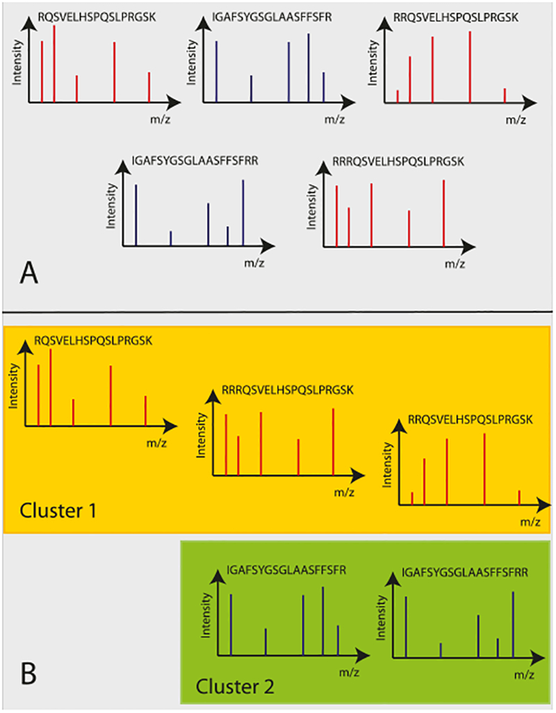
An example of spectral clustering. As shown in Section A of the figure, there are multiple spectra and each spectrum corresponds to a single peptide. Section B shows the clustered spectra. Note that, spectra that have been clustered together (shown with same color) correspond either to the same peptide (Cluster 2) or highly similar peptides with missed cleavages (Cluster 1).

3. Proposed CAMS-RS Algorithm

We exploit the spatial patterns in the mass spectrometry data to estimate the similarity of the spectra. The intuitive idea behind the similarity metric is that it is possible for noisy peaks to appear at random due to the stochastic nature of the mass spectrometry procedure which makes counting of common peaks between spectra for similarity assessment faulty. However, the probability that a group of consecutive peaks would appear in succession one after another for unrelated spectra is extremely low. Therefore, it makes more sense to group the consecutive peaks and use these groups as a source of comparison between spectra for similarity. We have defined a grouping method called F-set metric that makes sets of consecutive peaks present in the spectra. These sets are then compared with sets of other spectra and used as a similarity metric. The greater the number of sets that are common between the spectra, the more similar they are with respect to each other.

To determine the clusters in a given data set, an all-toall comparison is performed, i.e., each spectra is compared with every other spectra. All-to-all comparison may work for small numbers of spectra but it is not a scalable solution for large MS data sets. In order to deal with the scalability issues of the algorithm, we devised a strategy that allows restriction of search space, i.e., the potential number of spectra that have to be compared is greatly reduced. The search space restriction is a binning technique based on the precursor ion masses of individual spectra. Using this method, spectra with similar precursor ion masses (within a specified mass tolerance) are binned together. The binning decreases the number of comparisons by a order of magnitude and makes the clustering algorithm scalable. In order to merge the results from different bins, a merging strategy based on selective random sampling is formulated. The final clustering results are produced when the merging of cluster trees on individual bins is completed. The CAMS-RS algorithm is shown in Algorithm 1 and a high level figure is shown in Fig. 2. In the sections below we will discuss and formally define the individual parts of the algorithm.

Fig. 2.

Summary of CAMS-RS search space restriction and sampling.

3.1. F-Set Metric

A general strategy used by many clustering algorithms for mass spectrometry data is based on counting the common peaks between two given spectra (i.e.,”peak counting” methods) [1], [10]. It makes sense to count the number of peaks that may be common between the spectra due to the similarity of the corresponding peptide but there are potential problems, e.g., compounded spectra and noise can create false positives. A similarity metric that can mitigate these problems, enhance the peaks that are real and suppress the peaks that are not relevant to the similarity of the spectra, is essential for a dependable clustering algorithm [3], [22], [28], [33].

F-set metric is based on the observation that consecutive peaks in succession usually do not appear between two related spectra just by chance. Therefore it makes sense to estimate the similarity between two given spectra by comparing the consecutive sets of peaks. Since, the probability that consecutive sets of peaks would be common between spectra that are not related is almost zero, it has the potential to be a better similarity metric than individual peak counting techniques. The F-set metric was first introduced in [27] and we define here for the sake of completeness:

Definition 3. Let the spectra represented as S = {s₁, s₂,…, s_N}. Each spectra is a composite of m/z and intensity and the fragmentation spectrum can be formulated as s_j = (m₁, i₁), (m₂, i₂),…, (m_Q, i_Q) that is extracted from the mass spec-trometry data where m_d represents the m/z ratio and i_d represents the intensity of the peptide at position d and 1 ≤ j ≤ N. Now sets of peaks of size f are formed and can be represented as a vector F(s_i) = {(m₁m₂ ⋯ m_f), (m₂m₃ ⋯ m_f+1),…,(m_Q−f+1,…,m_Q−1, m_Q)}. The similarity metric callled F-set is calculated for two given spectra s_x and s_y as

$$W\left(s_x,s_y\right)={\displaystyle \sum _{i=1}^{\left|F\left(s_x\right)\right|}{\displaystyle \sum _{j=1}^{\left|F\left(s_y\right)\right|}\varphi \left(F\left(s_x\right)\left[i\right],F\left(s_y\right)\left[j\right]\right)}}$$ (1)

$$\varphi \left(a,b\right)=\{\begin{array}{ll}1\hfill & \text{if }a=b\hfill \\ 0\hfill & \text{o.w.}\hfill \end{array}$$ (2)

The numerical value of F-set metric for two given spectra is denoted by W(s_x; s_y). The F-set makes a set of m/z from the spectra of size f and then compares it with the F-set of the other spectra. If a match is established between a set from two spectra, a score of 1 is added. Otherwise a zero is added. Note that this scoring scheme can be changed according to the spectra being considered. According to the scoring scheme just defined, final weight score W represents the number of F-sets that are common between the two given spectra. In Fig. 3 three spectra are shown, out of which only two belong to the same peptide. As can be seen from the figure, using our definitions of F-set metric we are able to distinguish between the spectra that are related from the spectra that belongs to a different peptide. Now we briefly describe the graph-theoretic concepts used to design the algorithm.

Fig. 3.

Three spectra are shown in the figure. The first two spectra shown in A, D and B, E map to the same peptides whereas the third spectra shown in C, F belong to a different peptide. As can be seen in the figures A B and C that even though third spectra (C) is not similar to the first two spectra (A and B), there is a significant overlap between the spectra. However, if we make F-sets (of size 3 in this example) of the same peaks and spectra, it is clear that the sets formed do not have much in common for that spectra that is not related. The F-sets produced are: B → (b, d, f)(d, f, h)(f, h, l)(h, l, n), D →(b, d, f)(d, f, h)(f, h, j)(h, j, n) and F → (b, d, g)(d, g, l)(g, l, m)(l, m, n). It can be seen that after making F-sets, F do not have anything in common when compared to D and E, which have altogether different F-sets.

3.1.1. Graph Theoretic Framework

The algorithm creates a weighted undirected graph. Each spectrum is represented by a vertex and weighted edge represents the F-set weight metric calculated between two given spectra. More formally:

Definition 4. Let number of vertices V in a weighted undirected graphG = (V, E) are equal to the number of spectra S being considered, i.e., |V| = |S| = N and an edge E is used to connect each vertex. Now let a weight w_e=(vi,vj) ≥ 0 be associated with edge e = (v_i, v_j) where e ∈ E and v_i, v_j ∈ V. Each vertex is mapped to a spectra using the mapping function ∀v_i → s_i where v_i ∈ V, s_i ∈ S, 1 ≤ i ≤ N. Using equation 1, the weight on each edge is calculated for each pair of spectra, i.e., w_e = W(s_i, s_j) where e = (v_i, v_j); s_i, s_j ∈ S, e ∈ E, v_i, v_j ∈ V.

In accordance with the definition above, a weighted undirected graph is created where each vertex represents a spectrum, the edges represent the comparison between the spectra and the weight on the edges is calculated using the F-set metric definition provided in the text. After a complete weighted graph has been created, the next step is to extract the clusters out of the graph structure.

3.1.2. Extracting Clusters

In theory, after a complete weighted graph has been created (using F-set definitions and our scoring scheme) there must be two kind of edges. One type of edge(s) must have absolutely zero weights whereas other edges must be very highly weighted. Our experiments using high-resolution mass spectrometers suggest that even the spectra that do not correspond to the same peptide do get a small positive weight, albeit much smaller than the related spectra.

The reason for this small weight is the possibility of having b- and y-ions common between non-related spectra, e.g., although the spectra under consideration do not correspond to the same peptide, there might be parts of peptides that are common. Hence, not all of the spectra that are unrelated would get a zero or near-zero score. Therefore, one has to decide the minimum weight necessary for the edges to be considered as part of the cluster. The initial design of the algorithm [27] considered the use of support vector machines (SVM) to automate the process of selecting the threshold. However, we have found that selection of the threshold is far less complex than we suspected due to the large difference between the weights of related and non-related spectra. Our experiments with real data suggests that F-sets of size 7 or more and the spectra containing more than 30 set in common is enough to accurately determine the cluster membership. We have opted to make the selection of threshold ζ user-defined, where z is the minimum number of sets that must be common between two given spectra to classify them as clustered. Hence, for experimentation purposes and the default setting in our implemented code requires the user to define the threshold. A F-set of size 7 or more with weight of more than 30 seems to give a good tradeoff between accuracy and the number of clustered spectra (results not shown).

3.1.3. Connectedness in the Graph

Once the weight on the edges has been calculated and the algorithm eliminates all edges that have a threshold less than ζ. A forest of trees will be created till this stage using our intelligent matrix completion technique [25]. In order to determine which of the vertices are still connected, we used depth first search (DFS) which can run in O(m + n) time where m is the number of vertices and n is the number of edges [16]. As the final step, the vertices that are connected are reported as belonging to the same clusters.

3.2. Restricting Search Space and Sampling

The calculation of the F-set metric and extraction of clusters work well for a small number of spectra. However, similarity calculations that includes creation of F-sets from the spectra and comparison of these sets to other spectra is time-consuming. Further, all-to-all comparison of these F-set is not tractable with increasing number of spectra. For the algorithm to be scalable a more sophisticated method is needed that eliminates the need to compare every spectra with every other spectra. We have formulated two approaches that considerably narrow the search space and the number of comparisons the algorithm has to perform. A sampling strategy is adopted to further eliminate comparisons and complete the clustering results.

3.2.1. Horizontal Search Space Restriction

A mass spectrometer consists of three components: an ion source, a mass analyzer, and a detector. The ionizer converts a portion of the sample into ions. The differences in masses of the fragments allows the mass analyzer to sort the ions by their mass-to-charge ratio. The detector measures the value of an indicator quantity and thus provides data for calculating the abundances of each ion present. Some of these ions based on their mass-to-charge ratio are selected for further fragmentation. Now the spectra that have a similar mass are more likely to contain same peptides than the spectra that have very different masses, e.g., it is possible for spectra to be related, if they have close mass of 103 and 108, but it if far less likely that two of the spectra would be related if one has a mass of 1,000 and the other has a mass of 4,500. Therefore, close proximity of spectra mass may correspond to similar peptides and this becomes the basis of the horizontal space restriction. The peptides that have a same mass are more likely to correspond to a similar peptide than peptides with distant masses.

This becomes the basis of our horizontal search space reduction technique, i.e., all the spectra need not compared with all the other spectra. Only the spectra that have close mass will have peptides that are similar and potentially could be clustered. Therefore in our algorithm we select a range of mass and compare the spectra within that mass for potential clustering. A range of mass is used within a specified window to take into account peptides with missed cleavages and post-translational modifications.

In the algorithm the window of mass range is determined by the number of miss cleavages (M_C) and/or post-translational modification mass and ψ is the maximum number of allowed miscleavages or PTM’s. Therefore, mass range bins of size M_C ×ψ are formed for searching and comparing to other spectra. As can be seen in the Fig. 4 that only a small set of masses of the spectra are chosen to be compared with each other, decreasing the comparisons significantly.

Fig. 4.

Vertical and horizontal search space restriction is depicted for CAMS-RS. The x-axis represents the mass of the spectra and the vertical axis represents F-sets that have been generated. The highlighted part is the space that is searched for establishing the similarity of two given spectra.

3.2.2. Vertical Search Space Restriction

The masses in the data files from spectra are sorted in ascending order and have some order in which they can be compared. For the spectra that are related there would be some F-sets common between them. If there are absolutely no sets that are common between the spectra in early phases of the comparison, it is highly unlikely that F-sets with larger mass will have much in common between them. Therefore, it does not make sense to compare all F-sets between spectra. Our experiments have shown that comparing the first 10 F-sets of average size 7 is sufficient to establish if the spectra are related to each other or not. Initially, we compare the first 10 F-sets in CAMS-RS algorithm; if there are no matches, no further comparisons are performed. If some matches are positive in the early stage then comparisons of all F-sets are performed to ensure that consistent weight for the edges is calculated for the graph creation.

For two unrelated spectra Fig. 4 shows that only a few F-sets need to be compared and our strategy saves significant search space exploration and time. For the cases where there are F-sets that are common, the comparison is performed all the way (not shown in the figure) to establish a consistent weighting for the created trees. Since most of the comparisons between spectra will end up not being fruitful, Fig. 4 realistically depicts the vertical and horizontal search space reductions that are confirmed by our experiments later in the manuscript.

3.2.3. Sampling on Mass Bins

Once the restricted search space comparisons and pruning of the trees using the recommended z threshold have been performed, each of the bins would have (potentially) multiple cluster trees as shown in Fig. 2. Each of the trees in the bins represents a single cluster. Restricted search space has allowed the algorithm to determine clusters in each independent bin in an efficient manner. One consequence of this reduced search space is that trees on independent bins have not been explicitly compared. Hence, it is not known whether there are similar trees on the neighboring bins. Comparing all clusters in one bin with all clusters in other bins is computationally intractable.

A more efficient way to perform the comparisons across bins is using random sampling of the clusters. By definition each of the connect component is similar and the differences must be statistically insignificant, i.e., a randomly picked node on the tree would represent the whole population of the tree. Therefore, we pick random samples from each of the trees from independent bins that would represent the whole population of the data set. CAMS-RS algorithm is again applied to these spectra to determine similarity among them.

3.2.4. Merging Clusters Tree from Neighbouring Bins

The comparison of samples from neighbouring bins will reveal that some of the spectra are similar to other neigh-bouring spectra, i.e., there are spectra in a given bin that have similar spectra in a neighbouring bin. For the clustering results to be correct and complete, the spectra belonging to both trees must be merged together into one tree. We have a simple mechanism to merge the clusters.

If there is a sample that is similar to a neighbouring sample, the tree from which sample is extracted are brought into the neighbouring bin and merged with this tree (random edge merge). The clustering results are not effected by the topology of the resulting tree. The merged tree represents a single group in the final clustering result.

3.3. Load-Balancing Compute Bins

If there is a over-representation of a certain mass in the data set then a naive binning strategy does not remain scalable. The reason is that a over-representation of a certain mass in the data will force the algorithm to put more spectra in a single bin for comparison as compared to the number of spectra in other bins. The number of comparisons increases exponentially with increasing spectra and a more load-balanced approach is needed to keep the algorithm scalable. A limit on the number of spectra on a single bin is essential to keep the algorithm scalable.

Size of the bin is a design question that deals with a tradeoff between larger bin (gives large coherent clusters, but computationally is infeasible) and smaller bins (computationally efficient, but gives small clusters that require more sampling and merging). In order to empirically determine the maximum number of spectra per bin we analyzed spectra with same mass and varied the size of the bins. Our experiments have suggested that the number of spectra between 25 and 35 per bin works best (results not shown) both in terms of time and cluster size. The strategy allows us to keep the number of comparisons within a bin to a reasonable number and sampling/merging is also not extensive. The load-balancing scheme works fine in practice and the results with increasing number of spectra with and without load-balancing are shown in Fig. 5.

Fig. 5.

Observed wall clock time for non-balanced and load-balanced bins with increasing number of spectra.

4. Consensus of Clustered Spectra

Consensus from the clustered spectra has to be formed for further processing of the data. A correct consensus can be used for determining if clustering allowed us to mitigate some of the problems of incorrect searches of low S/N ratio spectra. A correct clustering and consensus spectra will allow us to compare clustered and consensus spectra against non-clustered spectra and see the potential advantages of our strategy. Further, use of consensus spectra would allow us to identify low S/N spectra and map them to correct peptides which would otherwise not be possible. In order for the consensus spectra to be useful for our purposes the consensus spectra created should be such that the real peaks are magnified and noise peaks are subdued. Note that clustering is applied to spectra before identification of peptides and for a given spectra there is no trivial way to distinguish between meaningful peaks and noisy peaks. Note that due to the stochastic nature of the peaks the consensus spectra created will only be advantageous if the spectra have been clustered correctly, i.e., if the clustering is incorrect then the consensus formed would be more nosier than the two individual spectra creating inaccurate search results. Since CAMS-RS is formulated in a way that the spectra that have common sets between them are more likely to be clustered than other spectra we can use this information to our advantage for creating consensus. The hypothesis is that the real peaks would survive in the consensus and the more random/noisy peaks would not be present at the same numerical mass-to-charge value.

In order to formulate the consensus we take two spectra that have been clustered together by CAMS-RS. Thereafter we select the peaks that are common between the two spectra. If the peaks are within 0.0005Da of each other they are considered to be the same peak and admitted in the consensus peak list. Other peaks are included in the exclusion list and are not included in the consensus spectra. In order to study what kind of consensus would work best we defined five kinds of criteria namely summation of the peaks, selection of minimum peaks, selection of maximum peaks, randomly selecting peaks for a given peak instance and average of the peaks under consideration.

We created clusters of experimentally generated data sets (see Experimental Methods). A consensus was formed for each of the clusters using the five criteria described above and the consensus was used for further processing. We found that there was no significant difference between the consensus strategy and all of them worked well for our purposes. Since, the spectra have been clustered accurately, any of the consensus strategies succeeded, i.e., real peaks were magnified and noisy peaks were eliminated. We use the average consensus strategy for our subsequent experiments and results.

5. Experimental Methods

We wanted to test our algorithm for different fragmentation strategies as well as for samples with different molarities. In order to test CAMS-RS algorithm for different fragmentation strategies we choose a CID and HCD data set from our paper [26]. A piece of freshly isolated rat liver was minced and sonicated in guanidine-HC1(6M, 3 ml). A peptide standard corresponding to the C-terminal sequence of the water channel Aquaporin-2 (AQP2) from rat, (Biotin-LC-CEPDTDWEEREVRRRQS*-VELHS*PQSLPRGSKA) phosphorylated at both S256 and S261 were added to 500 mg aliquots of liver sample (prior to trypsinization) with distinct amounts of 0:2nmol, 20pmol and 2pmol and were named AQP2-H-(S256/S261), AQP2-M-(S256/S261), AQP2-L-(S256/S261) respectively. The same procedure as above was repeated for another AQP2 peptide standard (Biotin-LC-CEPDTDWEEREVRRRQSVELHSPQS*LPRGSKA) phosphorylated at S264, with amounts of 0:2nmol, 20pmol and 2pmol and were named AQP2-H-(S264), AQP2-M-(S264), AQP2-L-(S264) respectively. Peptide samples were desalted, and then were suspended in 0:1 percent formic acid prior to analysis by mass spectrometry using HCD as well as CID fragmentation. The mass spectrometry raw data was then processed by the Sequest search engine to identify the peptides and used as a ground-truth data set for the quality assessment of the proposed algorithm. Please note that although we have used synthetic peptides, the data will also contain spectra corresponding to other peptides in the rat liver.

In order to make the quality assessment more comprehensive we also used Proteomics Dynamic Range Standard Set (UPS2) from Sigma-Aldrich to test our strategy. UPS2 can be used to standardize and evaluate LC-MS/MS and electrophoretic analysis conditions. The UPS2 contains a mixture of 48 individual human sequence recombinant proteins, each of which has been selected to limit heterogenous post-translational modifications. The protein standard is formulated from six mixtures of eight proteins to present a dynamic range of five orders of magnitude, ranging from 50pmol to 500amol. Briefly, 10.6 ug total protein (one vial) was resuspended in 50 ul of denaturation solution (8M urea, 50 mM Tris-HCl, 75 mM NaCl) followed by reduction and alkylation as previously described [12]. Protein samples were then digested with trypsin at a 1:20 (w/w) ratio for 16 h at 37°C. Peptides were then desalted (PepClean C-18 Spin Columns, Thermo Scientific) and eluted in 0:1 percent formic acid. Sample amounts of 10, 50, and 200 ng of digested peptides were analyzed on an LTQ Orbitrap Velos (Thermo Scientific), named as UPS-10, UPS-50 and UPS-200. Spectra were searched with Proteome Discoverer software (version 1.3.0.339, Thermo Scientific) running the Sequest algorithm on a concatenated database containing both the forward and reversed complement of the Rat Refseq Database (National Center for Biotechnology Information, March 3, 2010, 30,734 entries), which also included sequences for all human proteins included in the standard set UPS2, as well as a list of common contaminating proteins. Precursor ion tolerance was 25 ppm, whereas fragment ion tolerance was 1.0 Da. Three missed trypsin cleavage sites were allowed. Carbamidomethylation of cysteine (+57:021 Da) was added as a static modification. Variable modifications included oxidation of methionine (+15:995 Da) and deamidation of asparagine and gluta-mine (+0:984 Da). Known contaminant ions were excluded. The data sets were filtered to include < 1 percent false positive hits (estimated based on target decoy analysis [6].

These two data sets are then used as ground truths for quality assessment of the clusters and consensus obtained using CAMS-RS.

6. Performance Evaluation

The performance evaluation can be divided into two parts. The first part deals with quality of the clusters obtained using CAMS-RS and assessing the ability of clustering and consensus to improve the confidence of the identified peptides from low S/N ratio spectra. The second part deals with traditional performance metrics such as execution time with increasing size of data sets and memory requirements. First let us define the metric that we will use for quality assessment of the clusters. Thereafter, we introduce a quality assessment procedure in the next section for CAMS-RS algorithm.

If we just take an average of the individual quality of the cluster it may be misleading, since the number of elements in each cluster may be different. A metric has to be defined that represents the inter- as well as intra- quality of the clusters. Therefore, we have defined the accuracy as a weighted accuracy that allows us to determine the quality of the clustering for each cluster as well as the overall quality of all clusters. The weighted accuracy is defined as follows:

Assume there are k clusters and the accuracy of a single cluster i be denoted by a_i and the total number of spectra in the cluster be defined as n_i where 1 ≤ i ≤ k. Also assume that the number of spectra in a cluster that belong to the same peptide be denoted by x_i. Then, the accuracy of a single cluster can be defined as

$$a_i=\frac{x_i}{n_i},$$ (3)

and the average weighted accuracy (AWA) of the whole data set under consideration is defined as

$$AWA=\frac{{\displaystyle {\sum }_{i=1}^k{a}_i{n}_i}}{{\displaystyle {\sum }_{i=1}^k{n}_i}}.$$ (4)

As can be seen from the metric that AWA takes into account inter- as well as intra- accuracy of the clusters and gives a global view of the accuracy of the clusters obtained.

6.1. Quality Assessment

We use the following procedure to do the quality assessment:

1. Use the .raw data to search using Sequest algorithm against a concatenated rat and UPS2 protein database. The parameters illustrated in Section 5 are used for the search engine. The results that we get from Sequest are then used as ground truth data set.

2. Extract peak files (.dta) from .raw data and cluster them using CAMS-RS.

3. Execute average consensus strategy on the spectra that have been identified as clusters. The spectra that are not clustered as kept unaltered.

4. Create .mgf files from the clustered & consensus spectra and do the search again using Sequest with the same search parameters as stated in Section 5.

5. Compare the results from the previous step with the original Sequest results.

The quality assessment flowchart is presented in Fig. 6. Note that the clustering and consensus results are compared to Sequest search results. Sequest has approx accuracy of 70 percent when both high and low S/N ratio spectra are considered. Therefore, we will expect the most accurate clusters to have a AWA of around 70 percent since we do not expect Sequest to identify correct peptides from very low S/N ratio spectra which account for around 30 percent of the data in general [27]. The usefulness of clustering and consensus would be gauged by the ability of the algorithm to identify peptides with low S/N ratio spectra.

Fig. 6.

The flowchart of quality assessment procedure followed to assess the accuracy and effectiveness of the clustering algorithm.

6.1.1. Quality with Increasing F-Set Size

The objective of the first part of quality assessment is to see how the quality of the clustering relates to varying F-set size. Considering the framework that we introduced in the paper, the increasing size of F-set must correspond to higher accuracy. In order to confirm this, we choose CID and HCD data sets [26] discussed in the Section 5. We chose two AQP2 data sets for HCD and two for CID with high and low molarity samples.

Fig. 7 shows the average weighted accuracy with increasing size of the F-set. In general, the average weighted accuracy increases with increasing F-set size for both CID as well as HCD data sets. The accuracy reaches around 100 for F-sets of size 7 or more. The fact that accuracy increases significantly with increasing F-set size even for low molarity CID and HCD AQP2 data sets shows the effectiveness of F-set metric. The accuracy of the clusters using mixture of independently produced data sets is also shown in Fig. 7.

Fig. 7.

The average weighted accuracy is shown with increasing F-set size for CID as well as HCD data sets. ζ is constant at 30. The results are shown only for AQP2 peptides known to be in the sample. The key of the graph are: A = AQP2-H-(S256/S261)-HCD, B = AQP2-H-(S256/S261)-CID, C = AQP2-L-(S256/S261)-HCD, D = AQP2-L-(S256/S261)-CID. All data sets A, B, C, D are produced in independent experimental runs. The data is combined post-experiment to illustrate the usefulness of the algorithm for a combination of independently generated data sets.

In order to be consistent in presenting the results we cluster the rest of the data using size of F-set equal to 7 and ζ is constant at 30.

6.1.2. Quality with Different Fragmentation Methodologies

The AWA of the HCD and CID of AQP2 data is shown in Table 1. As can be seen in the table, the clustering algorithm allows high quality clustering for HCD as well as CID data sets even with varying experimental conditions. The clusters obtained are of very high quality, with near 100 percent accuracy. CAMS-RS was able to achieve near perfect accuracy even for the lowest molar amount of AQP2 peptide in the data set. These experiments illustrate that CAMS-RS is effective for different fragmentation methods and for varying molar amounts of peptide in the samples. Therefore the proposed clustering algorithm should be effective in a wide variety of real-world mass spectrometry data sets.

TABLE 1.

Summary of Results for HCD and CID Data Sets

CID datasets	No. of spectra	No. of clustered spectra	No. of clusters	AWA(%)
AQP2-H-(S256/S261)	2816	593	174	97.3
AQP2-M-(S256/S261)	2553	662	171	98.1
AQP2-L-(S256/S261)	2386	531	167	98.5
AQP2-H-(S264)	1842	485	153	98.7
AQP2-M-(S264)	1919	499	167	98.8
AQP2-L-(S264)	2163	490	166	96.3
HCD data sets
AQP2-H-(S256/S261)	2282	254	76	99.2
AQP2-M-(S256/S261)	2713	262	72	99.2
AQP2-L-(S256/S261)	2754	283	84	98
AQP2-H-(S264)	2060	132	44	98.5
AQP2-M-(S264)	2084	155	54	100
AQP2-L-(S264)	2267	164	57	100

The average size of the cluster and the average weighted accuracy of the data sets are shown.

6.1.3. Quality Assessment for Proteomics Dynamic Range Standard Set

We followed the quality assessment flowchart shown in Fig. 6 for Dynamic Range Standard Set (UPS2). Throughout our discussions we will use Sequest search results as a baseline against which CAMS-RS results would be compared. We use CAMS-RS to cluster this comprehensive data set with varying parameters and observing effects of clustering on its properties. After clustering and consensus we estimate the following parameters related to the data:

• 1)Varying the size of F-set and ζ and observing the average weighted accuracy and the number of spectra clustered: In order to see the accuracy of the clustering results, we changed the size of the F-set and the ζ, and ran the algorithm for UPS-10, UPS-50, and UPS-200. The average weighted accuracy with varying parameters is shown in Fig. 8. The average weighted accuracy of the clusters increases sharply with increasing size of F-set and z threshold. From the figure it can be observed, that bigger ζ translates to a increased accuracy. The variation in the accuracy is due to the increases and decrease in the ζ threshold, i.e., as can be seen from the figure, if the experiment was performed with constant F-set size, then with increasing z the accuracy would also keep on increasing. It is clear from the figure that the molarities and mixing of the independently produced data sets had minimal effect on the accuracy of the clusters. This is mainly due to the success of the F-set metric in recognizing noisy and random peaks and successfully utilizing real peaks for clustering. The sensitivity analysis is shown in Fig. 9.
• 2)Effect of clustering and consensus on Non-High (medium and low) and High-Confidence spectral matches: One of the potential advantages of clustering and consensus was to be able to make high confidence spectral matches for low S/N ratio spectra. In order to determine if the clustering had any effect on confidence with which a search engine can make a match, we clustered the spectra from UPS2 samples with varying F-set size and ζ. A consensus of the clustered spectra was formed and these consensus spectra were used for re-searching the data using Sequest. The results from sequest without C&C was used a base line. The results are reported in Fig. 10. As can be seen in the figure with increasing accuracy of the clusters, the number of spectra that can be matched with high-confidence increases drastically as compared with baseline Sequest search. Correspondingly, the number of peptides that get a lower- and/or -medium confidence match also decrease sharply with increased cluster accuracy as shown in Fig. 11.
• 3)Changes in peptide identification due to clustering, i.e., does clustering allow poor quality peptide matches to be matched to the correct protein: Clustering allows low S/N ratio spectra to be identified. By a similar argument it should also improve identification of spectra with high S/N ratio. A better identification of a peptide consists of two parts 1) correct identification of the peptide sequence and/or 2) correct identification of protein family where the peptide came from. If clustering has allowed better identification of a peptide then the probability that correct protein will be identified for this peptide is more likely. The results of protein grouping on the peptide is shown in Fig. 12. As can be seen in the figure, 64:7 percent of the peptides are not in the UPS2 family when only Sequest search engine is used. This includes both the high, medium and low confidence spectra matches. The number of peptides that do not belong to UPS2 protein families should be close to zero. In order to study the effect of clustering on peptide and protein identification we executed CAMS-RS algorithm on the UPS2 data set, formulated the consensus and ran the consensus spectra through Sequest. As can be seen in the Fig. 12, with increasing clustering accuracy the peptides that do not fall under UPS2 decreases sharply. For highest accuracy clusters the peptides that do not belong to UPS2 are close to 20 percent which is a significant improvement when compared with spectra that only have been searched using Sequest without clustering.

Fig. 8.

Quality of clustering with varying F-set size and threshold ζ. The graph shows the average weighted accuracy for different F-set size and ζ shown as x-axis parameters (F-set size, ζ). Note that the accuracy is calculated by comparing with Sequest search results. All data sets UPS-200, UPS-50 and UPS-10 are produced in independent experimental runs. The data is combined post-experiment to illustrate the usefulness of the algorithm for a combination of independently generated data sets.

Fig. 9.

The variation in sensitivity of the clustering results with varying F-set size and threshold ζ. The graph shows the sensitivity (percent) for different F-set size and z shown as x-axis parameters (F-set size, ζ).

Fig. 10.

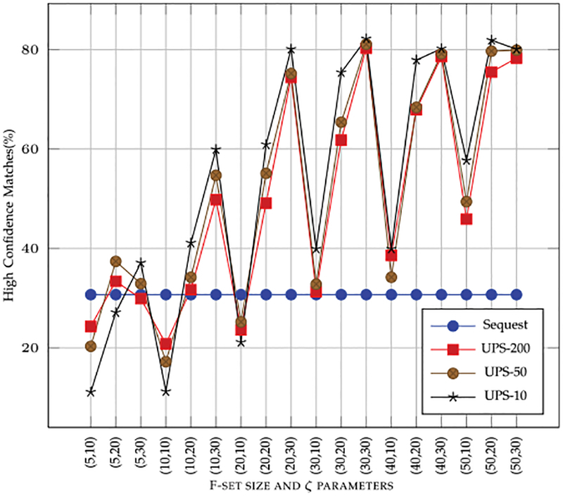
The effect of clustering with varying F-set size and threshold ζ on the number of high confidence matches for a said data. The high confidence matches using Sequest, without clustering, is also shown as a reference. The x-axis parameters are (F-set size, ζ).

Fig. 11.

The effect of clustering with varying F-set size and threshold ζ on the number of non-high (medium + low) confidence matches for a said data. The high confidence matches using Sequest, without clustering, is also shown as a reference. The x-axis parameters are (F-set size, ζ).

Fig. 12.

The effect of clustering with varying F-set size and threshold ζ on the number of number of peptides that are not part of the UPS2 protein family. The peptide matches to UPS2 proteins using Sequest, without clustering, is also shown as a reference. With increasing clustering accuracy, the number of peptides that are not part UPS2 decreases, i.e., more percentage of peptides get identified in UPS2 group. The x-axis parameters are (F-set size, ζ).

6.1.4. Quality with Multiple Independently Generated LC-MS/MS Data Sets

The use of retention time for clustering of mass spectrometry data has been proposed as a similarity metric. However, retention time is dependent on the particular analysis conditions, type of column, column dimension, degradation of column, existence of active points such as contamination, etc. The use of retention time as a useful similarity metric has been hindered by the variability of retention time even for identical columns or multiple runs of the same biological sample [15], [21].

We have designed CAMS-RS so that it can function independently and without considerations of non-linear shifts and variability of the retention times. This saves us from solving complex retention time problems within our clustering algorithm. This makes CAMS-RS a versatile tool that allows clustering of mass spectrometry data with varying experimental conditions, varying fragmentation methodologies and various independent runs of the biological sample. In order to illustrate the feasibility of such a clustering analysis we took our AQP2 and UPS2 data sets and mixed them together. Thereafter, CAMS-RS was run on the combined data sets. The mix of these data sets still allowed CAMS-RS to cluster data highly accurately as can be seen in Figs. 7 and 8. As can be seen that the quality of the clusters obtained is not effected by different experimental conditions or fragmentation methodologies of the data sets.

6.1.5. Comparing Quality with Other Clustering Tools

Two of the tools that are easily available for academic use are MS-Clust [10] and NorBel2 [9]. Like many other tools MS-Clust is based on normalized dot-product [10] and NorBel2 is based on sigmoid function. Sigmoid function is based on similarity of mass and intensity and is shown to perform better than simple dot-product metric [9]. Note that Sigmoid function is also based on single peak comparisons and spatial information in the peaks is not used for similarity assessment. Since it has been shown that sigmoid function is better than normalized dot-product, we will use NorBel2 for our quality comparisons.

In order to compare CAMS-RS and NorBel2 we used UPS2 data set that we have discussed in the manuscript. We calculate the AWA for CAMS-RS and NorBel2 and summarize in Table 2. A threshold of 50 (default) is set for NorBel2 which is shown to give good tradeoff between cluster size and accuracy [9].

TABLE 2.

Comparison of CAMS-RS and NorBel2 Using UPS2 Data Set

Data Set	NorBel2 AWA(%)	CAMS-RS AWA(%)
UPS-10	40.7	71.2
UPS-50	41.3	73.8
UPS-200	40.2	72.6

Threshold of 50 is set for NorBel2.

6.2. Complexity Analysis and Execution Time

The complexity analysis of the algorithm can be formulated as follows. For the sake of simplicity we will assume that the number of spectra is uniform across all masses, i.e., each mass gets equal number of spectra. Now let the total number of spectra be equal to N and average length of spectra be L. Then each of the steps of the algorithm will be as follows:

1. To sort the spectra requires T₁ = O(N + c) ≈ O (N) time using bucket or counting sort. In practice, best case performance should be expected since most of the peptide masses would be sorted coming out of mass spectrometer.

2. Number of bins created is equal to $B=\frac{M_{max}}{M_C\times \mathrm{\Psi }}.$

3. The number of spectra in each bin be equal to $n_B=\frac{N}{B^{\prime }}$ where n_B ≪ N.

4. To calculate F-sets and extracting clusters on each bin requires T₂ = O(n_B × L²) + O(V + E) = O(n_B ×L²) + O(n_B + n_B + 1).

5. Now let the number of trees on each bin be equal to k, and therefore the samples collected be equal to k from each tree. Also let the number of neighbours from whom samples are collected be equal to Q. The total number of samples collected from neighbouring bins that need to be compared is equal to Qk. Also the number of child bins created is equal to B/Q. Then the time to extract clusters from the child bins is equal to $T_3=\left(\frac{B}{Q}\times \left[\left(Qk{\left(L\right)}^2\right)+O\left(V+E\right)\right]\right)=\left(\frac{B}{Q}\times \left[\left(Qk{\left(L\right)}^2\right)+O\left(Qk+Qk+1\right)\right]\right).$

6. The other steps in the algorithm can be accomplished in constant time and is stated here as O(c) for the sake of simplicity.

Therefore, the total time complexity will be $O\left(T\right)=T_1+T_2+T_3=O\left(N\right)+O\left(n_B\times L^2\right)+O\left(2n_B+1\right)+O\left(\frac{B}{Q}\times \left(Qk{\left(L\right)}^2\right)\right)+O\left(\frac{B}{Q}\times \left(\left(2Qk+1\right)\right)\right).$ This expression can approximated to $T=O\left(N\right)+O\left(n_B\times L^2\right)+O\left(2n_B+1\right)+O\left(Bk{L}^2\right)+O\left(2Bk+\frac{B}{Q}\right).$ This can be further simplified as $T=O\left(N\right)+n_B{L}^2+B\left(k{L}^2+\frac{1}{Q}\right).$ Looking at the time complexity expression, it is clear that with increasing size of F-set the L² time will be dominant. The experimental results with increasing F-set size and increasing number of spectra is shown in Fig. 13. Note that F-set size of 7 or more will give clustering results close to 100 percent accuracy and increasing F-set beyond a certain number (8 or 9) does not have statistically significant effect on clustering accuracy. Therefore, a constant F-set size of 7 or 8 works best in practice and would give near-linear running times with increasing number of spectra. As can be seen from the complexity analysis that time required is very close to linear with increasing N with added fraction of time due to sampling and merging. For the constant F-set size, the time should increase linearly with increasing number of spectra. As can be seen in Fig. 14 that with increasing number of spectra, the time increases linearly and observed running time is very close to the theoretical time expected. We were able to cluster 1 million spectra in about an hour.

Fig. 13.

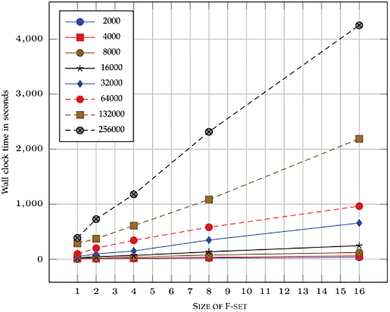
Wall clock time with increasing size of the F-set and number of spectra.

Fig. 14.

Wall clock time with increasing size of the data set with constant F-set size of 7.

7. Conclusions and Discussion

In this paper we have presented an efficient algorithm, called CAMS-RS, suitable for clustering of large-scale mass spectrometry data. A novel similarity metric (called F-set) is formulated and used in the algorithm based on the spatial locations and intensity of the peaks in a spectrum. The independence of the similarity metric from retention-time allows multiple sets of independently run LC-MS/MS experimental data sets to be clustered together. A graph-theoretic framework is introduced that allows the use of the introduced F-set metric in an efficient manner. In order to make the algorithm scalable with increasing number of spectra we introduce two different kind of search space restrictions. Each of the search space restriction dramatically decreased the search space for the algorithm while giving accurate clustering results. A sampling method is then introduced to merge the clustering results from different restricted search space (called bins).

A strategy to form consensus out of the clustered spectra was devised. The consensus spectra from these clustered data sets were then used for further computations such as identifying peptides from spectra, etc. Apart from the accuracy of the clustering results we were also interested in investigating the effects of clustering on identifying low S/N ratio spectra. We tested the accuracy of CAMS-RS using both CID and HCD data sets as well as experimentally produced synthetic data sets with known proteins. Using these experimentally generated data sets we showed that clustering of spectra using CAMS-RS allowed better identification of peptides and protein families when compared to spectra that were searched without clustering. The accuracy of the clustering results with varying parameters such as data set size, F-set size and z threshold are also presented in the paper.

Our complexity analysis suggests that time must increase linearly with increasing number of spectra. We experimentally showed that the time increases linearly with increasing number of spectra and clustering can be performed rapidly for large data sets. We were able to cluster a million spectra in about an hour on a modest workstation. The timing results with increasing data set size and with increasing F-set size are also presented in the manuscript and compared with theoretical times. We show a high quality implementation of our algorithm allows us to have near-linear runtimes with increasing number of spectra.

An algorithm with a novel similarity metric and scalable solution to clustering make CAMS-RS well suited for clustering of large-scale mass spectrometry data. The ability to create accurate clusters and representative consensus from these clustered results in a rapid fashion make it ideally suited for mass spectrometry analysis pipelines. The CAMS-RS algorithm allows interpretation of low S/N ratio spectra with much higher confidence when compared with non-clustered spectra. CAMS-RS also allows more accurate mapping of peptides to the protein groups. Thus, we believe that CAMS-RS is a very useful tool that can be used in conjunction with search engines to improve the peptide identification results and get more biological information from mass spectrometry data. We believe that the proposed algorithm will be immensely useful to the proteomics and mass spectrometry communities.

Require: MS2 spectra data set

Require: Number of miss cleavages M_C

Require: Mass of amino add with maximum Monoisotopic mass expected in the data Ψ

Require: Size of the F-set and the minimum cut-off threshold ζ

Ensure: Clusters of spectra such that the cluster has spectra that can be mapped to the same peptide:

• 1)Read the MS2 spectra and the associated
• 2)Enumerate the F-set of a given size for each of the spectra independently
• 3)Create bins of size M_C × Ψ and put spectra in these bins
• 4)Pick a spectra S_i from a bin and compare with the F-sets of other spectra in a bin
• 5)If the F-sets are more than ζ threshold, create an edge between the two spectra.
• 6)Keep doing the above step till all the spectra have been traversed and have obtained a tree membership or are unconnected
• 7)Randomly select samples from each bin from each tree that has been created.
• 8)Create new bins (child bins) with samples collected from the last step from neighbouring parent bins
• 9)Compare the F-sets of spectra in child bins and join them by edges if the F-set weight is more than ζ
• 10)If there are new edges in child bins, join those edges to the parent trees where the sample was extracted
• 11)Output the trees that have been created as clusters

Biographies

Fahad Saeed (S’05-M’10) received the BSc degree in electrical engineering from the University of Engineering and Technology, Lahore, Pakistan, in 2006 and the PhD degree in electrical and computer engineering from the University of Illinois at Chicago (UIC) in 2010. He is a research fellow in the Systems Biology Center at National Heart Lung and Blood Institute (NHLBI), National Institutes of Health (NIH) Bethesda, Maryland. His research interests include parallel and distributed algorithms and architectures, proteomics and genomics and parallel algorithms for bioinformatics applications. He is a member of the IEEE and ACM.

Jason D. Hoffert received the BSc degree in biology from Moravian College in Bethlehem, Pennsylvania, in 1997 and the PhD degree in biochemistry from the Johns Hopkins University School of Medicine in 2002. He was a postdoctoral fellow in the Laboratory of Kidney and Electrolyte Metabolism at NIH from 2002 to 2004. Since 2004, he has been a staff scientist in the Epithelial Systems Biology Laboratory at the National Heart Lung and Blood Institute in Bethesda, Maryland. He is currently using state-of-the-art phosphoproteomics methodologies to uncover the signaling pathways regulating kidney development and disease progression.

Mark A. Knepper received the BS degree in chemical engineering from the University of Michigan, 1970, the PhD degree in biomedical engineering from Case Western Reserve University (CWRU) in 1975, and the MD degree from CWRU in 1976. He is a biomedical engineer and systems biologist in the Intramural Program of the National Heart, Lung and Blood Institute (NHLBI) in Bethesda, Maryland. He has been an NHLBI scientist since 1978, focusing on mechanisms of water transport in the kidney and associ ated regulatory mechanisms. His current research involves large-scale integration of data from protein mass spectrometry, next-generation DNA sequencing, and the reductionist literature to identify mechanisms involved in regulation of trafficking and transcription of a molecular water channel called aquaporin-2.

References

- [1].Beer I, Barnea E, Ziv T, and Admon A, “Improving Large-Scale Proteomics by Clustering of Mass Spectrometry Data,” Proteomics, vol. 4, no. 4, pp. 950–960, 2004. [DOI] [PubMed] [Google Scholar]
- [2].Bensmail H, Golek J, Moody M, Semmes J, and Haoudi A, “A Novel Approach for Clustering Proteomics Data Using Bayesian Fast Fourier Transform,” Bioinformatics, vol. 21, no. 10, pp. 2210–2224, 2005. [DOI] [PubMed] [Google Scholar]
- [3].De Souza D, Saunders E, McConville M, and Likić V, “Progressive Peak Clustering in Gc-Ms Metabolomic Experiments Applied to Leishmania Parasites,” Bioinformatics, vol. 22, no. 11, pp. 1391–1396, 2006. [DOI] [PubMed] [Google Scholar]
- [4].Du X, Yang F, Manes NP, Stenoien DL, Monroe ME, Adkins JN, States DJ, Purvine SO, Camp DG II, and Smith RD, “Linear Discriminant Analysis-Based Estimation of the False Discovery Rate for Phosphopeptide Identifications,” J. Proteome Research, vol. 7, no. 6, pp. 2195–2203, 2008. [DOI] [PMC free article] [PubMed] [Google Scholar]
- [5].Dutta D and Chen T, “Speeding up Tandem Mass Spectrometry Database Search: Metric Embeddings and Fast Near Neighbor Search,” Bioinformatics, vol. 23, no. 5, pp. 612–618, 2007. [DOI] [PubMed] [Google Scholar]
- [6].Elias JE and Gygi SP, “Target-Decoy Search Strategy for Increased Confidence in Large-Scale Protein Identifications by Mass Spectrometry,” Nature Methods, vol. 4, no. 3, pp. 207–214, 2007. [DOI] [PubMed] [Google Scholar]
- [7].Eng JK, Fischer B, Grossmann J, and Maccoss MJ, “A Fast SEQUEST Cross Correlation Algorithm,” J. Proteome Research, vol. 7, pp. 4598–4602, Sept. 2008. [DOI] [PubMed] [Google Scholar]
- [8].Savitski MM, Lemeer S, Boesche M, Lang M, Mathieson T, Bantscheff M, and Kuster B, “Confident Phosphorylation Site Localization Using the Mascot Delta Score,” Molecular and Cellular Proteomics, vol. 10, no. 2, 2011, doi: 10.1074/mcp.M110.003830. [DOI] [PMC free article] [PubMed] [Google Scholar]
- [9].Flikka K, Meukens J, Helsens K, Vandekerckhove J, Eidhammer I, Gevaert K, and Martens L, “Implementation and Application of a Versatile Clustering Tool for Tandem Mass Spectrometry Data,” Proteomics, vol. 7, no. 18, pp. 3245–3258, 2007, doi: 10.1074/mcp.M110.003830. [DOI] [PubMed] [Google Scholar]
- [10].Frank AM, Bandeira N, Shen Z, Tanner S, Briggs SP, Smith RD, and Pevzner PA, “Clustering Millions of Tandem Mass Spectra,” J. Proteome Research, vol. 7, no. 1, pp. 113–122, 2008. [DOI] [PMC free article] [PubMed] [Google Scholar]
- [11].Fridman T, Razumovskaya J, Verberkmoes N, Hurst G, Protopopescu V, and Xu Y, “The Probability Distribution for a Random Match Between an Experimental-Theoretical Spectral Pair in Tandem Mass Spectrometry,” J. Bioinformatics and Computational Biology, vol. 3, no. 2, pp. 455–476, 2005. [DOI] [PubMed] [Google Scholar]
- [12].Hoffert JD, Pisitkun T, Saeed F, Song JH, Chou C-L, and Knepper MA, “Dynamics of the G Protein-coupled Vasopressin V2 Receptor Signaling Network Revealed by Quantitative Phosphoproteomics,” Molecular and Cell Proteomics, vol. 11, no. 2, 2012, doi: 10.1074/mcp.M111.014613. [DOI] [PMC free article] [PubMed] [Google Scholar]
- [13].Hoffert J, Pisitkun T, Wang G, Shen R, and Knepper M, “Quantitative Phosphoproteomics of Vasopressin-Sensitive Renal Cells: Regulation of Aquaporin-2 Phosphorylation at Two Sites,” Proc. Nat’l Academy Sciences USA, vol. 103, pp. 7159–7164, 2006. [DOI] [PMC free article] [PubMed] [Google Scholar]
- [14].Jiang X, Ye M, Han G, Dong X, and Zou H, “Classification Filtering Strategy to Improve the Coverage and Sensitivity of Phosphoproteome Analysis,” Analytical Chemistry, vol. 82, no. 14, pp. 6168–6175, 2010. [DOI] [PubMed] [Google Scholar]
- [15].Klammer AA, Yi X, MacCoss MJ, and Noble WS, “Peptide Retention Time Prediction Yields Improved Tandem Mass Spectrum Identification for Diverse Chromatography Conditions,” Proc. Ann. Int’l Conf. Research in Computational Molecular Biology, pp. 459–472, 2007. [Google Scholar]
- [16].Kleinberg J and Tardos E, Algorithm Design. Addison-Wesley Longman Publishing Co., 2005. [Google Scholar]
- [17].Molina H, Horn DM, Tang N, Mathivanan S, and Pandey A, “Global Proteomic Profiling of Phosphopeptides Using Electron Transfer Dissociation Tandem Mass Spectrometry,” Proc. Nat’l Academy Sciences of USA, vol. 104, pp. 2199–2204, 2007. [DOI] [PMC free article] [PubMed] [Google Scholar]
- [18].Moran MF, Tong J, Taylor P, and Ewing RM, “Emerging Applications for Phospho-Proteomics in Cancer Molecular Therapeutics,” Biochimica et Biophysica Acta (BBA) - Rev. on Cancer, vol. 1766, no. 2, pp. 230–241, 2006. [DOI] [PubMed] [Google Scholar]
- [19].Musbacher N, Schreiber TB, and Daub H, “Glycoprotein Capture and Quantitative Phosphoproteomics Indicate Coordinated Regulation of Cell Migration upon Lysophosphatidic Acid Stimulation,” Molecular & Cellular Proteomics, vol. 9, no. 11, pp. 2337–2353, 2010. [DOI] [PMC free article] [PubMed] [Google Scholar]
- [20].Nesvizhskii AI, “Computational and Informatics Strategies for Identification of Specific Protein Interaction Partners in Affinity Purification Mass Spectrometry Experiments,” Proteomics, vol. 12, no. 10, pp. 1639–1655, 2012. [DOI] [PMC free article] [PubMed] [Google Scholar]
- [21].Podwojski K et al. , “Retention Time Alignment Algorithms for Lc/Ms Data Must Consider Non-Linear Shifts,” Bioinformatics, vol. 25, no. 6, pp. 758–764, 2009. [DOI] [PubMed] [Google Scholar]
- [22].Powell D, Weaver C, Jennings J, McAfee K, He Y, Weil P, and Link A, “Cluster Analysis of Mass Spectrometry Data Reveals a Novel Component of Saga,” Molecular and Cellular Biology, vol. 24, no. 16, pp. 7249–7259, 2004. [DOI] [PMC free article] [PubMed] [Google Scholar]
- [23].Ramakrishnan SR, Mao R, Nakorchevskiy AA, Prince JT, Willard WS, Xu W, Marcotte EM, and Miranker DP, “A Fast Coarse Filtering Method for Peptide Identification by Mass Spectrometry,” Bioinformatics, vol. 22, no. 12, pp. 1524–1531, 2006. [DOI] [PubMed] [Google Scholar]
- [24].Saeed F, Hoffert J, Pisitkun T, and Knepper M, “High Performance Phosphorylation Site Assignment Algorithm for Mass Spectrometry Data Using Multicore Systems,” Proc. ACM Conf. Bioinformatics, Computational Biology and Biomedicine, pp. 667–672, 2012. [Google Scholar]
- [25].Saeed F, Hoffert JD, and Knepper MA, “A High Performance Algorithm for Clustering of Large-Scale Protein Mass Spectrometry Data Using Multi-Core Architectures,” Proc. Int’l Symp. Network Enabled Health Informatics, Biomedicine and Bioinformatics (HIBI-BI), Aug. 2013. [Google Scholar]
- [26].Saeed F, Pisitkun T, Hoffert JD, Wang G, Gucek M, and Knepper MA, “An Efficient Dynamic Programming Algorithm for Phosphorylation Site Assignment of Large-Scale Mass Spectrometry Data,” Proc. IEEE Int’l Conf. Bioinformatics and Biomedicine Workshops (BIBMW), pp. 618–625, 2012. [DOI] [PMC free article] [PubMed] [Google Scholar]
- [27].Saeed F, Pisitkun T, Knepper MA, and Hoffert JD, “An Efficient Algorithm for Clustering of Large-Scale Mass Spectrometry Data,” Proc. IEEE Int’l Conf. Bioinformatics and Biomedicine (BIBM), pp. 1–4, 2012. [DOI] [PMC free article] [PubMed] [Google Scholar]
- [28].Slotta D, Heath L, Ramakrishnan N, Helm R, and Potts M, “Clustering Mass Spectrometry Data Using Order Statistics,” Proteomics, vol. 3, no. 9, pp. 1687–1691, 2003. [DOI] [PubMed] [Google Scholar]
- [29].Tabb DL, MacCoss MJ, Wu CC, Anderson SD, and Yates JR, “Similarity among Tandem Mass Spectra from Proteomic Experiments: Detection, Significance, and Utility,” Analytical Chemistry, vol. 75, no. 10, pp. 2470–2477, 2003. [DOI] [PubMed] [Google Scholar]
- [30].Tabb DL, Thompson MR, Khalsa-Moyers G, VerBerkmoes NC, and McDonald WH, “Ms2grouper: Group Assessment and Synthetic Replacement of Duplicate Proteomic Tandem Mass Spectra,” J. the Am. Soc. for Mass Spectrometry, vol. 16, no. 8, pp. 1250–1261, 2005. [DOI] [PubMed] [Google Scholar]
- [31].Whitelegge JP, “HPLC and Mass Spectrometry of Intrinsic Membrane Proteins,” Methods in Molecular Biology, vol. 251, pp. 323–340, Dec. 2003. [DOI] [PubMed] [Google Scholar]
- [32].Yan B, Pan C, Olman VN, Hettich RL, and Xu Y, “A Graph-Theoretic Approach for the Separation of B and Y Ions in Tandem Mass Spectra,” Bioinformatics, vol. 21, no. 5, pp. 563–574, 2005. [DOI] [PubMed] [Google Scholar]
- [33].Zheng H, Anand S, Hughes J, and Black N, “Methods for Clustering Mass Spectrometry Data in Drug Development,” Proc. Fifth Int’l Workshop Intelligent Data Analysis in Medicine and Pharmacology, p. 4, 1998. [Google Scholar]