Enhancements to AERMOD’s Building Downwash Algorithms based on Wind-Tunnel and Embedded-LES Modeling

Abstract

Knowing the fate of effluent from an industrial stack is important for assessing its impact on human health. AERMOD is one of several Gaussian plume models containing algorithms to evaluate the effect of buildings on the movement of the effluent from a stack. The goal of this study is to improve AERMOD’s ability to accurately model important and complex building downwash scenarios by incorporating knowledge gained from a recently completed series of wind tunnel studies and complementary large eddy simulations of flow and dispersion around simple structures for a variety of building dimensions, stack locations, stack heights, and wind angles. This study presents three modifications to the building downwash algorithm in AERMOD that improve the physical basis and internal consistency of the model, and one modification to AERMOD’s building pre-processor to better represent elongated buildings in oblique winds. These modifications are demonstrated to improve the ability of AERMOD to model observed ground-level concentrations in the vicinity of a building for the variety of conditions examined in the wind tunnel and numerical studies.

1. Introduction

High ground-level concentrations (GLCs) from stack effluent present a potentially negative impact on human health; therefore, knowing the path and fate of a stack plume is a critical part of human health risk assessments. Pollutant emissions from elevated stacks within the complex and turbulent flow region around buildings and other structures can have a greater impact on ground-level concentrations near the release point than they would in the absence of a building. AERMOD, a steady-state Gaussian-type dispersion model that takes into account local meteorology, source characteristics, and complex terrain, as well as the presence of nearby structures, predicts the physical motion (e.g., plume rise and dispersion) of a plume in the near-field (Cimorelli et al., 2005). PRIME (Plume Rise Model Enhancements) is the building downwash algorithm within AERMOD that accounts for the influence of a building on the flow and dispersion of the plume (Schulman et al., 2000).

Previous evaluations of AERMOD in building downwash situations show varied performance, with the model doing well against observations in some cases (e.g., Petersen and Carter, 2006, and Olesen et al., 2009) but poorly in others (e.g., Petersen et al., 2017; Schulman and Scire, 2012). One of the goals of the work reported here is to evaluate the performance of AERMOD (with PRIME) against large datasets from wind tunnel and computational fluid dynamics (CFD) studies to identify and assess problem areas, such as discontinuities, and then to develop algorithm improvements within the general framework of the original PRIME approach. At this stage, only single, rectangular buildings are considered, with the reasoning that removing any shortcomings that arise in these relatively simple cases will add to the reliability of the algorithms in more complex situations, such as industrial complexes.

Comparisons of AERMOD to the Thompson wind tunnel dataset by Olesen et al. (2009) show that AERMOD has a tendency to under-predict ground-level concentrations for cases where the rooftop stack height exceeds the building height. Specifically, for stack height of 1.5H , AERMOD repeatedly falls short of capturing the magnitude of the building downwash, thus under-estimating the ground level concentrations near the building, for cubical, wide, and long buildings (Olesen et al., 2009). However, for cases where the stack matches the building height, Olesen et al. (2009) show that the modeled concentrations for certain building dimensions can greatly exceed the observed ones near the building.

While Olesen et al. (2009) found that the model under-predicted for a building with a 1.5H stack and a relatively large length in the along wind direction, others have found that significant over-predictions can occur with buildings of similar aspect ratios (Petersen et al., 2017; Schulman and Scire, 2012). Petersen et al. (2017) attribute the over-prediction to several aspects of the methodology behind AERMOD. For one, they argue that the uniform increase in turbulence intensity throughout the height of the wake region creates too much eddy- driven dispersion in the upper wake when wind tunnel data show turbulence intensity peaking near and just above the building height. Enhanced turbulence intensity throughout the wake could bring more effluent to the ground, thereby creating over-predictions (Petersen et al., 2017). And de Melo et al. (2012) discuss that AERMOD fails to reproduce the lateral shift in the plume for oblique wind conditions.

Relevant field or laboratory data addressing many of these specific areas of criticism had not been available, previously, for driving the development of improved algorithms. This paper is the third in a series reporting on an ongoing project to improve the performance of the building downwash algorithm. Two studies - a wind tunnel study (Perry et al., 2016) and complementary large eddy simulation (LES) study (Foroutan et al., 2018) – provide the basis for improvements to AERMOD. This paper reports on four specific changes: 1) improvement to the transition of plume material moving from the cavity into the far wake regions; 2) specification of an effective velocity that is more appropriate for diffusion estimates within the building wake; 3) modifications to the expressions for wake turbulence that more accurately reflect the original formulations of Weil (1996) upon which the wake model is based; and 4) a simple modification to the building preprocessor program for oblique wind angles. Finally, a comparison of results from both the current and modified versions of AERMOD against the recent wind tunnel and LES results are discussed.

2. Building Downwash

The interaction of an atmospheric boundary layer with an obstacle can have a significant effect on the flow field in the vicinity of that obstacle. If there is an effluent release within that disturbed flow region, the dispersion of the effluent plume can be vastly different from that without the obstacle. This effect often results in an elevated plume being brought to the ground rapidly and is referred to as building downwash. The interaction of the flow with the obstacle or building changes with the amount of upwind turbulence, the atmospheric stability, and physical characteristics of the obstacle. Generally, the following characteristics are observed: 1) a wake region in the lee of the structure, consisting of disturbed flow that extends far beyond the object, 2) a near-field wake of recirculating flow close to the structure, and 3) streamline deflection upward and downward in the upwind and downwind, respectively, regions of the structure. Flow separation occurs at the corners of sharp-edged structures leading to pockets of low pressure and reverse flow at various locations around building. In the lee of the building, high turbulence intensity and reverse flow characterize the dynamic near-wake region, which is often referred to as the “cavity” (Fig. 1).

Figure 1.

Near- and far-wake boundaries (dotted lines), as computed by AERMOD shown for a 1:1:2 building of height H. The plume trajectory as determined by the streamline algorithms is also shown (gray line). Both downwind and vertical distances have been normalized by H.

For a cubical building, a little over half of an approaching flow will move over the cube and the remaining will move around, as part of a large horseshoe vortex that wraps around the building to a reattachment point at thedownwind extent of the cavity (Hussein and Martinuzzi, 1996). For 3D, sharp-edged structures, the recirculation length, defined as the distance to the downstream reattachment point of the leading wall horse-shoe vortex, is short relative to those for 2D buildings (Fackrell, 1984), which arises from the fact that a large amount of flow goes around the building (Martinuzzi and Tropea, 1993). Castro and Robins (1977) noted that a reduction in incoming turbulence extends the reach of the cavity (see also Castro and Steggel, 1999). The cavity length then grows more slowly with building width $(W)$ after about W = 8H, where H is the building height (Martinuzzi and Tropea, 1993; Fackrell, 1984; Hosker, 1981, 1984). Any stack effluent that gets trapped in this near-wake is eventually transported into the far wake, as instabilities from interactions with roof-flow periodically destabilize the arching vortex tube at the leeward wall (e.g., Fackrell, 1984; Sousa, 2002). The expansive downwind wake region is less dynamic than the cavity, its expanse grows slowly (Martinuzzi and Tropea, 1993), and it is characterized by negative vertical velocity and enhanced turbulence intensity.

As AERMOD is a steady-state model, the intermittent and time-variable position of the vortices that surround a blunt object in a wind field are not captured. Instead, a time-averaged picture of the effluent field is modeled. AERMOD does this through many algorithms, but four main components can be isolated and are explained infurther detail below. The first component reviewed here is stream-line deflection. AERMOD creates building- specific streamlines to reflect observations from wind tunnel studies of flow around buildings. Along with other physical processes such as buoyancy-driven plume rise, the streamline field is then used to adjust the path of the plume centerline. Second, to handle the splitting of the plume into different flow regions, such as the near and far wakes, AERMOD creates two new sources and redistributes the mass among the three sources, each with their own Gaussian distributions in z and y (σ_z and σ_y ,respectively) that vary downwind, along the x-axis. Third, a dependence of turbulence intensity on x and on a few constants deduced from wind tunnel data serves as a basis for the calculations of σ_z and σ_y (Weil, 1996). Lastly, a preprocessor called BPIPPRM reduces the complexity of building structures for all incoming wind angles, and, for each wind direction, presents AERMOD with a single building perpendicular to the wind.

2.1. Streamline Deflection

Incoming air will be deflected above and around a building that it encounters, and the dispersion of nearby effluent is dependent, among other things, on the building dimension and angle at which the oncoming wind encounters the upwind face of the building. Streamline descent in the lee of the building is one of the dominant causes of high ground-level concentrations resulting from a stack above the building. While the effects of the building on the streamlines diminish with downwind distance and height, the steeper streamlines act to bring down effluent for any part of the plume within the wake’s area of influence.

Schulman et al. (2000) split the streamline field in AERMOD into five regions: 1) an upwind, unaffected region;2) the near-field, upwind region; 3) the sharp ascent over the building; 4) a region traversing the top of the building and descending in the lee; and 5) the recovery within the far wake. The streamline slopes depend on three building-defined quantities: the maximum height of the rooftop cavity, H_R, the along-wind length of the near-wake, L_R, and the building dimensions, the latter of which is summed up in the wake length scale, defined as $R=B_S^{2/3}{B}_L^{1/3}$, where BS is the smaller of the along-wind length and crosswind width dimensions and BL is the longer of the two dimensions. The maximum height of the rooftop cavity also depends on the building length scale through the relation $H_R=H+0.22R$, where the upwind edge is located at x = ,0 if there is no streamline reattachment to the building. The length of the near-wake is an empirically-derived expression based on Fackrell (1984), who built upon earlier work by Hosker (1981):

$$L_R=\frac{1.8W}{\left[{\left(\frac{L}{H}\right)}^{0.3}\left(1+0.24W/H\right)\right]}$$ 1

where L is the downwind length of the building. AERMOD does not model streamlines within the cavity and,instead, treats this region differently, as discussed below.

In addition to a near-wake boundary that contains the recirculating flow in the lee of a building, AERMOD designates a far-wake boundary that specifies the extent of the region of building influence (Fig. 1). The building’s influence decreases with increasing vertical distance above the building, manifested as streamline slopes approaching zero. The bounding curve for the far-wake region, which is based, in part, on the “free wake” formulation by Schlichting (1968) and which Schulman et al. (2000) derived by combining t wo empirically-formulated dependencies of building dimensions on wake height, is given as $H_W=1.2R{\left[H/R+{\left(H/1.2R\right)}^3\right]}^{1/3}$. Any stack effluent within this bounding curve gets passed to the building downwash routines within AERMOD, with the model treating the remainder of the plume as it would in the absence of a building.

2.2. Plume Partitioning

AERMOD handles the recirculation region in the lee of a building by creating two sources, in addition to the primary plume source, and splitting up the effluent mass between the three (Schulman et al., 2000). The primary plume contains the mass that is not captured in the cavity. The two additional sources represent the amount of effluent trapped in the near-wake (cavity source) and the amount that is released from the cavity to the far field (re-emitted source). The distance over which the cavity source is present depends on the physical dimensions of the cavity at a specific height. In the along-wind dimension, this contribution tapers linearly with downwind distance from 0.85L_R until 1.15 , after which only the re-emitted plume and/or the primary plume contribute to the receptor concentration (Fig. 2). While the cavity source contribution is decreasing, the re-emitted source contribution is increasing at the same rate, and the sum of all the source emission rates, at any given location, is equal to the total emission rate.

Figure 2.

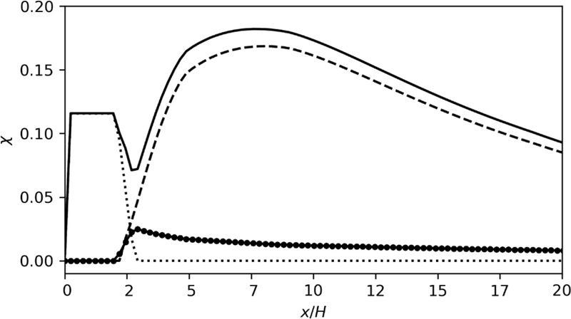
Downwind, normalized GLC (χ) at y = 0 shown versus normalized downwind distance (x / H). The separated sources (cavity source (···), re-emitted source (∙ −), and primary source (- -)) and total (−) contributions are shown. The lee wall is located at x = 0, and the end of the cavity is located at approximately 2.24H.

2.3. Wake Turbulence

In the lee of a building, fluctuations in the lateral and vertical velocity components, σ_v and σ_w, respectively, become important, growing in magnitude relative to the wind speed. These increased turbulence intensities, i_y = σ_v/U and i_z = σ_w/U, enhance plume spreading. The growth of the plume dimensions (σ_y and σ_z) are found by integrating the turbulence intensity (i_y for lateral growth, i_z for vertical growth) over the downwind distance, x. To ascertain the enhanced turbulence intensity within a building wake, AERMOD first simplifies the problem by splitting the system into short-term and long-term scales (Weil, 1996), with the point between the two determined by the estimated time at which a parcel of air loses the initial velocity it gained while in the well-mixed region in the lee of the building. This time scale, t_d, is proportional to the ratio of the characteristic building length scale to the upstream wind speed.

For time less than t_d, large motions from mechanical mixing will dominate as air flows over and around the building. Thus, for t < t_d, it is assumed that the distribution of a pollutant follows a Gaussian probability density function (PDF) of a parcel’s vertical (p_z) and lateral (p_y) position, such that the vertical Gaussian function, for example, varies in x and is based on $\overline{w}$, the mean, or effective, downwash wind speed (Weil, 1996). An expression for σ_W comes from the integration of dz_p/dx where z_p is the plume height, with the assumption that U and σ_w vary in x from the upstream values as U =U0 − ∆U (x), and that ∆σ_w and ∆U decrease in x as x^−2/3, as is the case for a “free wake” (Weil, 1996). Weil (1996) assumes vertically invariant values of ∆σ_w and ∆U within the wake to arrive at an expression for vertical turbulence intensity, i_z, as follows, assuming that x_R = (x + R − L )⁄R is a building-scaled downwind distance:

$$\begin{gathered} i_z=\frac{{\sigma }_w}{U}=\frac{{\sigma }_{w0}+\Delta {\sigma }_{w0}{x}_R^{-2/3}}{U_0-\Delta U_0{x}_R^{-2/3}} \\ =i_{z0}\left[1+\frac{\frac{\Delta {\sigma }_{w0}}{{\sigma }_{w0}}+\frac{\Delta U_0}{U_0}}{x_R^{2/3}-\left(\Delta U_0/U_0\right)}\right] \\ =i_{z0}\left[1+\frac{\left(\frac{1.7i_{zN}}{i_{z0}}-1\right)+\frac{\Delta U_0}{U_0}}{x_R^{2/3}-\left(\Delta U_0/U_0\right)}\right] \end{gathered}$$ 2

where i_z0 = σ_w0/U₀ and the factor 1.7 arises from estimates taken from wind tunnel data: ΔU₀/U₀ = 0.7, a maximum vertical turbulence intensity in the lee of approximately i_z ≈ 0.3, and i_zN ≈ 0.06. In this PDF region, σ_z will vary as ${\sigma }_z(x)={\displaystyle \int i_{z}dx}\text{'}$, with i_z given in Equation 2.

Downwind of the PDF region is the eddy diffusivity region, where, again according to Weil (1996), σ_z varies in xas $d{\sigma }_z^2/dx=2K_z/U$, such that:

$$\begin{gathered} {\sigma }_z(x)=\sqrt{{\sigma }_{z,x_d}^2+{\displaystyle \int \frac{2K_z}{U}}dx\text{'}}=\sqrt{{\sigma }_{z,x_d}^2+\left(x-x_d\right)\frac{2K_1{\sigma }_w(x)h_w(x)}{U(x)}} \\ =\sqrt{{\sigma }_{z,x_d}^2+\left(x-x_d\right)\frac{2{\sigma }_{z,x_d}}{h_{w,x_d}}{i}_z(x)h_w(x)} \end{gathered}$$ 3

where K_z is the vertical eddy diffusivity, the proportionality constant, k₁, is a ratio of vertical scales of motion at the transition point, t = t_d, and x_d is the downwind distance to t_d. Effectively, with a decrease in enhanced turbulence intensity, the rate of growth of σ_z is lower in the eddy diffusivity region than it is in PDF region. This trend matches wind tunnel data from Perry et al. (2016) and LES data from Foroutan et al. (2018) that show enhanced turbulence intensity throughout the wake but higher values within the cavity, particularly at the outer cavity boundary (results not shown here).

2.4. BPIPPRM Effective Building Dimensions

BPIPPRM (Building Profile Input Program for PRIME) is the building preprocessor program that provides the effective building dimensions to AERMOD for each source and wind direction. AERMOD requires that the building be specified as rectangular and perpendicular to the incident flow; therefore, for each source and wind direction combination, BPIPPRM assesses and simplifies the surrounding collection of buildings to provide a single effective building with an upwind wall perpendicular to the prevailing winds. A single building significantly simplifies the simulation of the building downwash problem. BPIPPRM’s methodology of defining the effective building is based upon good-engineering-practice (GEP) stack height guidance (USEPA, 1985) to ascertain if any particular building or collection of buildings would likely influence the effluent plume from a nearby stack. In determining the effective building dimensions for oblique winds as a single rectangular building, BPIPPRM defines the projected building length and width as the distance between the along- and cross-stream extremities, respectively. This particular aspect of BPIPPRM will be discussed further in Section 4.4. Once the effective building dimensions, orientation, and location relative to the stack(s) have been determined for each wind direction, this information is passed to AERMOD for the flow and dispersion calculations.

3. Downwash Datasets

A recent extensive wind tunnel study (Perry et al., 2016) and associated large eddy simulation modeling (Foroutan et al., 2018) of building downwash around a range of rectangular buildings have provided the basis for a clearer understanding of the dominant features of pollutant dispersion in these complex and turbulent flow situations. This has allowed for a fresh examination of the performance of the AERMOD dispersion model and the development of improvements to AERMOD’s building downwash algorithms.

3.1. Wind Tunnel Study

A wind-tunnel study described by Perry et al. (2016) examined a range of building aspect ratios, source heights and locations, and approach wind directions relative to the building. The study was performed at a scale of 1: 150 with buildings of various size but always 150 tall (a full-scale equivalent of 22.5 ). Building height ( ) is used throughout to normalize the building dimensions, source height and concentrations. The wind tunnel was set up with an approach boundary layer designed to simulate conditions in a suburban or light-industrial area using Irwin spires (Irwin,1981) to initialize the development of a simulated atmospheric boundary layer. The flow is further conditioned with an array of tabs (each 38 high, 76 wide, and 1 thick) spaced 305 apart in both the streamwise and cross-stream directions such that each successive row is offset laterally from the previous one by 152.5, producing a staggered pattern. The resulting boundary layer had a full-s cale equivalent roughness length of 0.36 m with a displacement height of 0 m. The reference wind speed (U₀) in the tunnel was held at 2.77 m s⁻¹ at building height, and the friction velocity of the approach flow was 0.25 m s⁻¹.

The cases studied in the wind tunnel include three building aspect ratios (L : W : H = 1: 1: 2, 1: 1: 4, and 1: 1: 8, where L = streamwise length, fixed at 150 mm, W = cross-stream width), five wind directions (θ = 0°, 15°, 30°, 45°, and 60°), three source heights (1.2H , 1.5H , and 2.0H ), and four source locations around the perimeter of the building. The source locations were the middle of the downwind face of the building (DM0), the middle of the upwind face of the building (UM0), the downwind corner of the building (DC+), and the upwind corner of the building (UC−) (see Fig. 3).

Figure 3.

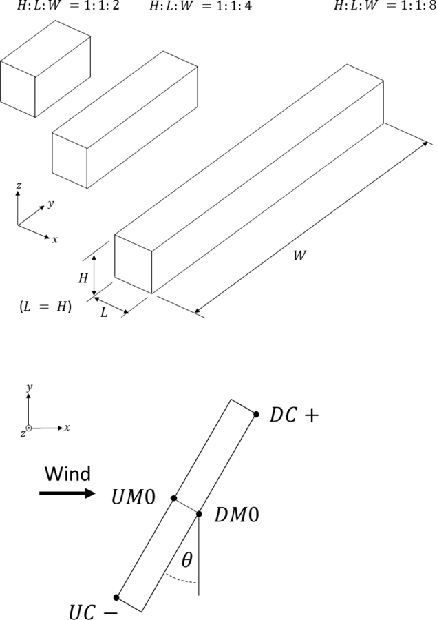
Above: The different building dimensions and notations used in the wind tunnel and ELES studies. Below: Wind angle or building rotation is shown along with the different stack locations used in the studies (UM0: upwind middle center; DM0: downwind middle center; DC+: downwind corner at positive-y end; and UC-: upwind corner of the building at the negative-y end).

During experiments, a neutrally buoyant tracer material (ethane, whose molecular weight is within 0.4% of that of air) was released from a source consisting of a 7mm diameter porous plastic ball. The resulting concentration patterns were characterized using Rosemount Model 400A hydrocarbon analyzers (flame ionization detectors) by sampling throughout the tunnel. Mean velocity and turbulence measurements were performed using laser Doppler velocimetry. For both concentration and velocity measurements, signals were sampled at 20Hz over 120 s periods.

To facilitate comparison between wind-tunnel, LES, and dispersion modeling results, all concentrations are normalized as χ=C/C₀ with $C_0=\frac{Q}{H^2{U}_0}$, where C is the background-adjusted concentration, U₀ is the reference wind, and Q is the tracer gas emissions rate.

3.2. Large-Eddy Simulation

Embedded Large Eddy Simulations (ELES) were performed for six of the cases from Perry et al. (2016) to provide greater detail in the spatial and temporal variations in the velocity, turbulence, and concentrations fields (Foroutan et al., 2018). Denoting the cases with their aspect ratio, wind direction, stack height, and stack location, the six cases simulated were: 1: 1: 2 − 0° − 1.5H− 0, 1: 1: 2 − 45° − 1.5H − 0, 1: 1: 8 − 0° − 1.5H − 0, 1: 1: 8 − 45° − 1.5H −0, 1: 1: 2 − 0° − 1.5H − +, 1: 1: 2 − 0° − 1.2H − 0. The region of the flow surrounding the building and including the near-wake was simulated using LES with a domain of size 11H in the streamwise direction, 3H vertically, and 6H laterally (12H for the 1: 8 building). Surrounding this LES region was a larger area domain where RANS (Reynolds Averaged Navier-Stokes) simulations were performed. The RANS domain had a stream-wise length of 32 , a height of 8.9H , and a lateral width of 24.7H . The LES zone began 5H downwind of the inlet to the RANS zone and was centered laterally. In addition, the LES zone extended from the ground, and the building was located 3H downwind of the inlet to the LES zone.

The turbulence closure was the Wall-Adapting Local Eddy-Viscosity (WALE) model in the LES region (Nicoud and Ducros, 1999) and two-equation Shear Stress Transport (SST) k-ω model in the RANS area with a turbulent Schmidt number of 0.7. A two-dimensional vortex method developed by Mathey et al. (2006) was used to generate a time-dependent, perturbed condition at the RANS-LES interface. The top and side boundary conditions include zero normal velocity and zero normal gradients of all other variables. The outflow uses zero static pressure and zero gradient conditions, and no-slip conditions were applied at the building, stack, and ground boundaries.

The computation grid was well-resolved near the building (cell size 0.028 ) with further refinement in the vicinity of the source and stack (0.0035H ). The cell size grew with distance from the building to a size of 0.05H in the LES zone and to 0.44H in the RANS zone. Time-averaged flow quantities were o btained by averaging the LES simulations over a time period equal to 15 through-flow times for the domain, corresponding to 105 computational time steps (∆t_∗ = U₀ ∆t/H = 0.00615).

The results of the numerical simulations compared favorably to the wind tunnel simulations (see Foroutan et al.(2018) for a more complete description of the numerical simulations and their comparison to the wind tunnel results).

4. Modifications to Building Downwash Algorithms

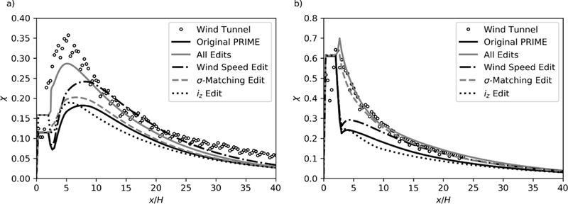
As discussed in Section 1, AERMOD has received criticism for over-predicting ground-level concentrations in some building downwash situations. However, other studies (e.g., Perry et al., 2016; Olesen et al.,2007) have found that for the simple case of a 1: 1: 2 building with a 1.5H stack located at the downwind middle of the building with oncoming orthogonal winds, AERMOD under-predicts ground-level concentrations throughout much of the wake, reaching only halfway to the peak observed ground-level concentration (Fig. 4). This under- prediction compared to wind tunnel data repeats for stacks at various locations on the building, for 1.2H tall stacks, and for varying wind directions (Fig. 4).

Figure 4.

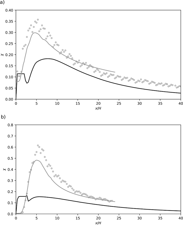
a) Downwind, longitudinal profiles at y = 0 of wind tunnel (o), ELES (−), and AERMOD (−) GLCs for a 1:1:2 building with a stack positioned at DM0 and incoming winds at an angle of 0°. b) GLC profiles as above but for 45° winds. The maximum ground level χ increases for this case (note the vertical scale difference) when the winds are no longer orthogonal to the upwind wall; however,AERMOD fails to model the extent of the increased downwash.

As discussed in Section 2, AERMOD simulates the downwash effect using a three-plume approach. For example, Equation 4 shows the total ground-level concentration as calculated by AERMOD, with the cavity, re-emitted, and primary plume contributions given by the first, second, and third terms, respectively:

$$\begin{gathered} C_{PRIME}=\frac{3\left[\lambda fQ\right]}{H_{C}W{\text{'}}_B{U}_H}{e}^{\left[-\frac{1}{2}{\left(\frac{y}{{\sigma }_{yc}}\right)}^2\right]}+\frac{\left[\left(1-\lambda \right)fQ\right]}{\pi {\sigma }_{yc}{\sigma }_{zc}{U}_S}{e}^{\left[-\frac{1}{2}{\left(\frac{y}{{\sigma }_{yc}}\right)}^2\right]} \\ +\frac{\left[\left(1-f\right)Q\right]}{\pi {\sigma }_y{\sigma }_z{U}_S}{e}^{\left[-\frac{1}{2}{\left(\frac{H_p}{{\sigma }_z}\right)}^2\right]}{e}^{\left[-\frac{1}{2}{\left(\frac{y}{{\sigma }_y}\right)}^2\right]} \end{gathered}$$ 4

where the scaling factor, λ, decreases linearly from 1 to 0 as x increases from 0.85L_R to 1.15L_R, λ is the fraction of the plume captured by the cavity, U_S is the wind-speed at the stack height, H_c is the maximum cavity height, and U_H and W′_B are the building height wind-speed and plume mixing width scale, respectively (Schulman et al.,2000). At any given point in space, not all terms necessarily contribute to the PRIME component of the concentration – the amount each source contributes depends on the x, y, and z location of a given receptor.

The next sub-sections pinpoint potential shortcomings of the building downwash algorithms that contribute to previously reported poor model results and describe model changes that increase model consistency and address some of the problems outlined therein.

4.1. Plume Spread Matching

AERMOD creates a cavity source and a re-emitted source for the component of the plume caught in the recirculation in the lee of the building and bases the downwind plume growth on the work of Weil (1996). AERMOD determines the fraction of mass (λ in Equation 4) for the cavity source as the part of the plume that crosses the physical boundaries of the cavity. The cavity σ_y and σ_z are defined by the cavity’s physical size; therefore, as x increases, the diffusion coefficients in the cavity remain constant, such that the concentration along a specified height is invariant in x. On the other hand, the sigma values for the re-emitted plume and the primary plume grow with downwind distance, and the amount of growth conditionally depends on its downwind distance to determine if a parcel of air still has a “memory” of the highly turbulent near-wake (see Section 2.3 above).

One problem identified in the modeled longitudinal GLCs arises from the calculation method for σz and σy. A large decrease in ground-level concentration downwind of the lee edge of the cavity (Fig. 2) occurs when the contribution of cavity plume to the overall concentration starts to wane, the primary plume contributes little to the total concentration, and the re-emitted plume dominates. The effects of plume partitioning along with large vertical and lateral diffusion for the re-emitted plume relative to the cavity plume together manifest as low concentrations at the ground. If the effluent caught in the cavity moves downwind to create the re-emitted plume,then having the two Gaussian plumes match at the edge of the cavity would make the handoff smoother. In fact,AERMOD matches the Gaussian σ_y and σ_z for the re-emitted and cavity plumes, but the matching location occurs at the lee wall of the building, with the re-emitted plume growing in x from that point. Moving this matching point from the lee side of the building to the lee edge of the cavity (Fig. 5) and allowing the re-emitted plume to grow from there, removes the dip in GLCs seen in the figure. This change improves the continuity of the model and removes a seemingly nonphysical dip in the time-averaged concentration. This modification also increases the GLCs just downwind of the cavity, which also effectively reduces the downwind distance to the maximum concentration.

Figure 5.

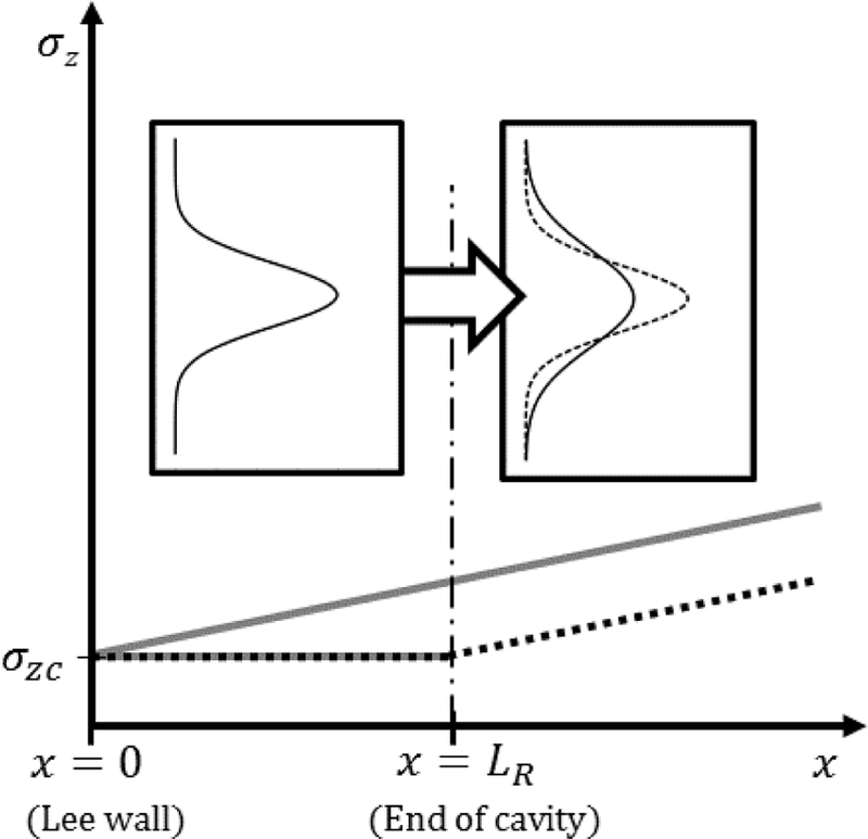
The growth of σ_z for the re-emitted plume. The solid line shows the growth from the lee wall (original algorithm). The dotted line shows the new pattern, where σ_z for the re-emitted and cavity plume, σ_zc, match at the end of the cavity, x = LR. Inset: the vertical concentration profile within the cavity (left panel); the profile after plume is emitted from the cavity (solid line, original; dotted line, revised).

4.2. Wind Speed

In addition to plume dispersion, wind speed contributes to the Gaussian concentration calculation as part of the flux component. Utilizing the appropriate wind speed for each of the three regions of the building effected plume is particularly important. The AERMOD downwash algorithm currently uses the wind speed at stack height for the primary plume. This likely results in an under-estimate of GLCs in the lee of a building where longitudinal wind speeds drop and vertical motions gain relative importance. As used elsewhere in AERMOD, an effective wind speed, U_eff, defined from the upwind wind speed profile as the speed vertically averaged from a receptor height to the plume centerline, would better capture the actual winds influencing the plume in the region downwind of the building. In this way, U_eff appropriately scales with any changes in the ambient wind speed profile resulting from changes in upwind roughness or atmospheric stability, for example. Employing this change in AERMOD has the effect of increasing GLCs within the wake, as the wind-speed decreases within lower portion of the profile. Similarly, for the re-emitted plume, the wind speed at stack height is replaced with a more representative one at the building height to create a smoother transition between the cavity and re-emitted plumes.

4.3. Turbulence Levels

As stated earlier, AERMOD bases the computation of the vertical and lateral dispersion coefficients on formulations of Weil (1996). The theory states that, within the wake, the turbulence intensity enhancement decays as x^−2/3 from a peak value at the leeward wall of a building. To simplify the formulation, all the deviations within the wake from the lee wall values are taken to be vertically invariant, and the values of the reductions are estimated from wind tunnel data. When originally implemented in PRIME, the maximum value of the ambient turbulence intensity was reduced from Weil’s value of 0.07 to 0.06. PRIME uses this constant as an upper limit, choosing it over the turbulence intensity calculated from the effective parameters at 15R when the latter is higher. The larger maximum ambient turbulence intensity value better reflects the simulated atmosphere of wind tunnels as reported by Weil (1996); however, this value would not likely represent more extreme atmospheric conditions, in particular, very stable ones. While a method to address extreme stabilities might warrant further consideration, implementing this higher ambient turbulence intensity in AERMOD only raises the minimum possible value. Making this change has the expected effect of bringing the plume down more quickly and, therefore, reducing the downwind distance to the maximum GLC. A maximum GLC located closer to the leeward wall of the building brings the model closer to resembling the recent wind tunnel and ELES data (Fig. 4).

4.4. BPIPPRM

In addition to combining nearby buildings into an effective single one, or choosing the most influential building for a particular stack and wind direction, the AERMOD building preprocessor program, BPIPPRM, provides for enhanced building dimensions when the wind is at oblique angles to a side of a rectangular structure. BPIPPRM takes the longitudinal and lateral extremities of a rotated (with respect to the winds) building and uses the distance between the two to form the effective building length and width, respectively (dotted lines in Fig. 6). For an elongated building and large oblique wind angles, BPIPPRM substitutes a building that can have a large footprint in relation to the actual building that in turn may have an unrealistically large impact on the streamlines and wake parameterizations in AERMOD.

Figure 6.

Projected building using the new BPIPPRM algorithm (dark gray) shown with the corresponding physically rotated building (light gray) and original BPIPPRM projected building (--) for 15°, 30°, 45°, and 60° relative winds, if the winds are moving from left to right.

To address this issue in BPIPPRM, one possible alternative effective length can be defined from the path that an air parcel actually travels in a straight path across the building rather than from the longitudinal extremities of the rotated building, reducing the size of the projected building (dark gray rectangles in Fig. 6). The building width calculation remains unchanged from the original BPIPPRM method, and the center of the projected building is located at the center of the rotated building. Reducing the effective building length reduces the size of the near-wake recirculation region by decreasing the value of L_R in Equation 1, which in turn changes the streamlines and, ultimately, the plume trajectory.

5. Model Evaluation

Each change to AERMOD’s building downwash algorithm affects the modeled GLCs. For the case presented in Fig. 7a (1: 1: 2 − 0° − 1.5H − DM0), the modifications to the model resulted in an increase in the GLC estimates within the cavity of about 30%, while, for the case in Fig. 7b ( 1: 1: 2 − 0° − 1.2H − DM0 ), the model changes have little effect on the cavity concentrations.

Figure 7.

Normalized ground-level concentrations along y = 0 verses downwind distance shown for a stack height of 1.5H (a) and 1.2H (b), as measured in the wind tunnel (Perry et al., 2016) (○) and modeled by AERMOD, both the original (—) and modified (—) model. The algorithm changes are shown separately (∙− use of Ueff and UH for the primary and re-emitted plumes, respectively; --use of the σz-matching between the cavity and re-emitted plumes; and ··· use of the greater minimum value of the ambient turbulence intensity), for the purpose of showing how each affects the ground-level concentration.

For further comparison to the wind tunnel database of Perry et al. (2016), the model is evaluated using the maximum values of the two downwind, lateral concentration profiles taken at x = 3H and x = 10H. Comparing the maximum of the model and wind tunnel lateral profiles (χ_max,AERMOD versus χ_max,WT, respectively) for orthogonal winds across all building dimensions, stack locations, and building aspect ratios, the original AERMOD model tends to under-predict the observed values, with several points falling below the lower factor-of-two line (Fig. 8a). With the changes to AERMOD outlined here, a similar analysis shows that more data fall within the factor of two bounding lines and shows less bias toward under-prediction, suggesting that the model better captures the peak concentrations along those lateral profiles (Fig. 8b).

Figure 8.

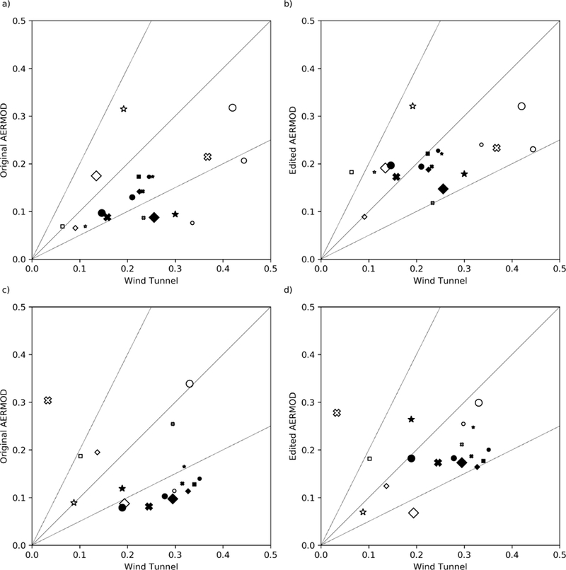
Maximum normalized ground-level concentrations plotted for the model versus wind tunnel at 0(a-b) and 45°(c-d) winds. The maxima are taken from lateral profiles at two downwind locations, x = 3H and 10H. Shown on the left are the results using the original model, and, on the right, the results with changes outlined in Section 4. The solid and dashed lines are the 1:1 and factor-of-two lines, respectively. (Stack location symbols are as follows: o: DM0, ✖: UM0; ♦: UC-; ★: DC+. Open symbols: x = 3H; closed x = 10H. Small symbols: 1:1:2 aspect building ratio; medium-sized symbols: 1:1:4; large symbols: 1:1:8).

In the case of orthogonal winds, the BPIPPRM changes have no influence on predicted concentrations. Instead, the changes in Fig. 8b come from algorithm changes for plume spread matching, use of an enhanced ambient turbulence intensity, and the use of an effective wind-speed and building-height winds over the wind-speed at stack height. An examination of the cases for an incoming wind angle of 45° (Fig. 8c) reveals an even greater tendency of the original AERMOD to under-predict (documented in Perry et al., 2016). Incorporating the proposed BPIPPRM changes along with the others just mentioned, more of the AERMOD results fall within the factor of two bounding lines and show less bias toward under-prediction; however, two outliers persist for the 1: 1: 8 building with stack locations at UCC − and UM0 (Fig. 8d).

Statistical measures useful for characterizing model performance include fractional bias (FB) and normalized mean square error (NMSE), defined as (modified from Chang and Hanna, 2004):

$$FB=\left(\frac{\overline{C_p}-\overline{C_o}}{0.5\left(\overline{C_o}+\overline{C_p}\right)}\right)$$ 5

and

$$NMSE=\frac{\overline{{\left(\overline{C_o}-\overline{C_p}\right)}^2}}{\overline{C_o}\overline{C_p}}$$ 6

where C_p and C_o are the predicted and observed data, respectively. For this lateral profile dataset, the overbars denote an average of the lateral maxima across both downwind distances and other possible degrees of freedom, i.e., stack height, stack location, wind direction, and building aspect ratio. The modified model shows an improvement in fractional bias and reduced NMSE, with respect to the original AERMOD, across all of the wind angles (Fig. 9). Similar improvements from the original AERMOD to the modified versions of AERMOD and BPIPRM are observed when comparing FB and NMSE across the different building aspect ratios and source locations (not shown here). When combined, the modifications proposed here show substantial improvement in the ability of AERMOD to capture the peak GLC, the downwind location of the maximum GLC, and the qualitative shape of the concentration profile as compared to the wind tunnel data.

Figure 9.

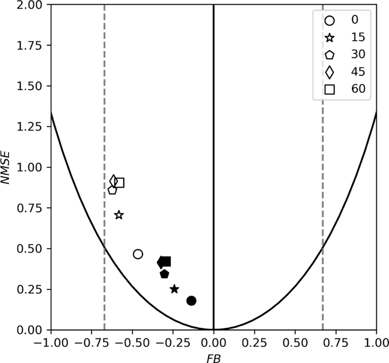
NMSE versus FB against wind tunnel data for the original model (open symbols) and model with algorithm changes (closed symbols). The modified model has a lower NMSE and FB across the building dimensions, stack locations, and stack heights at the various wind angles (see inset legend).

Both the qualitative and statistical assessments suggest that the current algorithm modifications are moving the model towards more accurate predictions of building downwash. Reductions to fractional bias and model variations are seen across all the building dimensions, wind directions, stack heights, and stack locations surveyed in the wind tunnel (Perry et al., 2016) and ELES studies (Foroutan et al., 2018). While the modified AERMOD is able to capture the maximum concentrations at specific downwind distances, additional changes are required for AERMOD to capture the full extent of the observed lateral shifts in the plume for oblique wind angles relative to the upwind wall of a building.

6. Conclusion and Future Areas of Research

The goal of this study was to use newly acquired experimental and numerical building-downwash data to improve the ability of AERMOD to accurately model these important and complex dispersion situations. Changes in AERMOD’s building downwash algorithm that improve continuity and internal, theoretical consistency bring model simulations closer to replicating wind tunnel data. Changes to the model have been made to add continuity across the edge of the cavity by equalizing the dispersion coefficients for the cavity and re-emitted sources, to employ a better characteristic velocity for the concentration calculation for the re-emitted and primary sources, and to increase the minimum ambient vertical turbulence intensity back to that suggested by Weil (1996). In addition, the preprocessor program for establishing an effective building shape for oblique wind angle was altered to reduce the effect of wind angle on the projected building footprint. Results from these changes bring the longitudinal ground-level concentration profiles closer both in shape and magnitude to those of the wind tunnel data. Additionally, analyses show that there is less bias and statistical spread in the model results, and these improvements occur across the various building aspect ratios, on-coming wind angles, stack heights, and stack locations examined in this study.

It is important to note that both the wind tunnel measurements and numerical simulations were conducted in a neutral atmospheric boundary layer. While the effects of atmospheric stability on building wakes were not considered in these studies, Robins (1994) suggests that building downwash concepts applicable to neutral flows can be extended to moderate departures from the neutral state. Additionally, stable towing tank experiments on cubical buildings have shown that concentration patterns in building wakes were insensitive to building Froude numbers (Fr), except under very stable (Fr < 2.5) conditions (Snyder, 1994).

The changes to the downwash algorithms within AERMOD and to BPIPPRM presented here produce encouraging results, but more modifications are warranted in order to address persisting issues. Specifically, in its current state, AERMOD lacks the ability to replicate the extent of lateral plume shifts observed in the wind tunnel and ELES data for non-orthogonal winds, and the near- and far-wake boundaries may need to be reduced in order to lessen plume entrainment into these regions. Using wind tunnel and ELES data, new algorithms can be developed to alter the various components of the modeled plume in order to simulate lateral shifts and other complexities in the plume trajectory that are dependent on wind direction, stack location, and building dimensions. The plume partitioning method used in the building downwash algorithms of AERMOD depends critically on the size and shape of the building cavity; therefore, improved algorithms are needed to better predict the boundaries of the cavity, particularly for the oblique wind cases. Also, algorithm improvements are needed to simulate the enhanced streamline deflection that occurs as a result of the strong corner vortices that form in oblique winds. Lastly, while the modifications presented here improve model performance under a variety of wind and building configurations, further insight could be gained from extending these analyses to comparisons against full-scale field studies.

References

- Castro IP and Robins AG, 1977. The flow around a surface-mounted cube in uniform and turbulent streams,J. Fluid Mech, Vol. 79 Part 2, 307–335. [Google Scholar]
- Castro IP and Steggel N, 1999. Effects of stable stratification on flow and dispersion around a cube, Wind engineering into the 21st century: proceedings of the tenth International Conference on Wind Engineering: Balkema, Rotterdam, 1725–1730. [Google Scholar]
- Chang JC and Hanna SR, 2004. Air quality model performance evaluation, Meteorol. Atmos. Phys, Vol. 87, 167–196. [Google Scholar]; Cimorelli AJ, Perry SG, Venkatram A, Weil JC, Paine RJ, Wilson RB, Lee RF, Peters WD, and Brode RW (2005). AERMOD: A dispersion model for industrial source applications. Part I: general model formulation and boundary layer characterization, J. of Applied Meteorol, Vol. 44, 682–693. [Google Scholar]
- de Melo AMV, Santos JM, Mavroidis I, and Reis NC Jr., 2012. Modelling of odour dispersion around a pig farm building complex using AERMOD and CALPUFF. Comparison with wind tunnel results. Building and Environment, Vol. 56, 8–20. [Google Scholar]
- Fackrell JE, 1984. Parameters characterizing dispersion in the near wake of buildings. J. Wind Eng. Indus. Aerodyn, Vol. 16, 97–118. [Google Scholar]
- Foroutan H, Tang W, Heist DK, Perry SG, Brouwer LH, Monbureau EM, 2018. Numerical analysis of pollutant dispersion around elongated buildings: an embedded large eddy simulation approach. Submitted to Atmospheric Environment. [DOI] [PMC free article] [PubMed] [Google Scholar]
- Hosker RP, 1981. Methods for estimating wake flow and effluent dispersion near simple block-like buildings, NOAA Technical Memorandum, Silver Spring, MD. [Google Scholar]
- Hosker RP, 1984. Flow and diffusion near obstacles, in: Randerson D (Ed.) Atmospheric Science and Power Production, Springfield, VA: National Technical Information Service, pp. 241–326. [Google Scholar]
- Hussein HJ and Martinuzzi RJ, 1996. Energy balance for turbulent flow around a surface mounted cube placed in a channel, Physics of Fluids, Vol. 8, 764−780. [Google Scholar]
- Irwin HPAH, 1981. The design of spires for wind simulation. J. Wind Eng. Indus. Aerodyn, Vol. 7, 361–366. [Google Scholar]
- Martinuzzi R and Tropea C, 1993. The flow around surface-mounted, prismatic obstacles placed in a fully developed channel flow, J. Fluids Eng, Vol. 115, 85–92. [Google Scholar]
- Mathey F, Cokljat D, Bertoglio JP, and Sergent E, 2006. Assessment of the vortex method for large eddy simulation inlet conditions. Prog. Comput. Fluid Dyn. Int. J, Vol. 6, 58–67. [Google Scholar]
- Nicoud F and Ducros F, 1999. Subgrid-scale stress modelling based on the square of the velocity gradient tensor. Flow, turbulence and Combustion, Vol. 63, 183–200. [Google Scholar]
- Olesen HR, Berkowicz R Ketzel M, and Løfstrøm P, 2009. Validation of OML, AERMOD/PRIME and MISKAM Using the Thompson Wind-Tunnel Dataset for Simple Stack-Building Configurations, Boundary-Layer Meteorol, Vol. 131, 73–83. [Google Scholar]
- Perry SG, Heist DK, Brouwer LH, Monbureau EM, and Brixley LA, 2016. Characterization of pollutant dispersion near elongated buildings based on wind tunnel simulations, Atmospheric Environment, Vol. 42, 286–295. [Google Scholar]
- Petersen RL and Carter JJ, 2006. Evaluation of AERMOD/PRIME for two sites with unusual structures, 99th Annual Conference of the Air & Waste Management Association. [Google Scholar]
- Petersen RL, Guerra S, and Bova A, 2017. Critical review of the building downwash algorithms in AERMOD, Journal of Air & Waste Management Association , Vol. 67, 826–835. [DOI] [PubMed] [Google Scholar]
- Robins A, 1994. Flow and dispersion around buildings in light wind conditions, in: Castro and Rockliff (Eds.) Stably Stratified Flows. Flow and Dispersion over Topography, Institute of Mathematics and its Applications Conference Series, Oxford: Clarendon Press, pp. 335–358. [Google Scholar]
- Schlicting H, 1968. Boundary-Layer Theory, New York, NY: McGraw-Hill. [Google Scholar]
- Schulman LL, Strimaitis DG, and Scire JS, 2000. Development and evaluation of the PRIME plume rise and building downwash model, Journal of Air & Waste Management Association, Vol. 50, 378–390. [DOI] [PubMed] [Google Scholar]
- Schulman LL and Scire JS, 2012. Building downwash modeling with AERMOD, 10th Conference on Air Quality Modeling: RTP, NC. [Google Scholar]
- Snyder WH, 1994. Some observations of the influence of stratification on diffusion in building wakes, in: Castro and Rockliff (Eds.) Stably Stratified Flows. Flow and Dispersion over Topography, Institute of Mathematics and its Applications Conference Series, Oxford: Clarendon Press, pp. 301–334. [Google Scholar]
- Sousa JMM, 2002. Turbulent flow around a surface-mounted obstacle using 2D-3C DPIV. Exp. in Fluids, Vol. 33, 854–862. [Google Scholar]
- U. S. Environmental Protection Agency, 1985. Guideline for Determination of Good Engineering Practice Stack Height: (Technical Support Document for the Stack Height Regulations) USEPA, Office of Air and Radiation, Office of Air Quality Planning and Standards, Research Triangle Park, NC, EPA-450/4–80-023R, 101 pp. [Google Scholar]
- Weil JC, 1996. A new model for stack sources in building wakes, Ninth Joint Conference on Applications of Air Pollution Meteorology with the Air & Waste Management Association: Boston, MA, 333–337. [Google Scholar]