Automatic Recognition of fMRI-derived Functional Networks using 3D Convolutional Neural Networks

Abstract

Current fMRI data modeling techniques such as Independent Component Analysis (ICA) and Sparse Coding methods can effectively reconstruct dozens or hundreds of concurrent interacting functional brain networks simultaneously from the whole brain fMRI signals. However, such reconstructed networks have no correspondences across different subjects. Thus, automatic, effective and accurate classification and recognition of these large numbers of fMRI-derived functional brain networks are very important for subsequent steps of functional brain analysis in cognitive and clinical neuroscience applications. However, this task is still a challenging and open problem due to the tremendous variability of various types of functional brain networks and the presence of various sources of noises. In recognition of the fact that convolutional neural networks (CNN) has superior capability of representing spatial patterns with huge variability and dealing with large noises, in this paper, we design, apply and evaluate a deep 3D CNN framework for automatic, effective and accurate classification and recognition of large number of functional brain networks reconstructed by sparse representation of whole-brain fMRI signals. Our extensive experimental results based on the Human Connectome Project (HCP) fMRI data showed that the proposed deep 3D CNN can effectively and robustly perform functional networks classification and recognition tasks, while maintaining a high tolerance for mistakenly labelled training instances. Our work provides a new deep learning approach for modeling functional connectomes based on fMRI data.

I. Introduction

Inferring functional brain networks from FMRI data has become a popular method to better understand human brain functions recently. Typically, dozens or hundreds of concurrent functional brain networks can be effectively and robustly reconstructed from whole brain functional magnetic resonance imaging FMRI data of an individual brain using independent component analysis ICA [1]–[5] or sparse representation [6]–[12]. For instance, by using the online dictionary learning and sparse coding algorithm [13], several hundred of concurrent functional brain networks, characterized by both temporal time series and spatial maps, can be decomposed from either task based FMRI (tFMRI or resting state FMRI (rsFMRI data of an individual brain [14 ]. Pooling and integrating the spatial maps of those functional networks from many brains can significantly advance our understanding of the regularity and variability of brain functions across individuals and populations [15]. For example, by clustering hundreds of thousands of functional brain networks from Autism Spectrum Disorder (ASD patients and healthy controls, our recent work identified 1 group-wisely common intrinsic connectivity networks (ICNs shared between ASD patients and healthy control subjects, where some ICNs are substantially different between the two groups [15]. Specifically, spatial map of the default mode networks ICN and fusiform gyrus activation ICN are found to have decreased connectivity in patient group than control group after statistical test. The atypical patterns of those ICN maps between two groups brought insight into the investigations of the spatial maps of the reconstructed networks from the original fMRI images. In general, quantitative mapping of spatial maps of functional networks across individuals and populations offers a very powerful way to understand the brain functions in healthy brains and their alterations in brain disorders [14], [16], [17].

However, pooling and integration of spatial maps of functional networks across individuals and populations is not an easy task. Here, we briefly introduce our own experiences in attempting to accurately and robustly aggregate spatial network maps across multiple brains. In our earlier effort of developing the Holistic Atlases of Functional Networks and Interactions (HAFNI system [6], [11], [14], 23 task-invoked group wise consistent networks and 10 resting state networks were identified and confirmed by manual visual inspections, assisted by simple temporal and spatial similarity metrics such as Pearson correlations of time series and overlaps of spatial maps. Though this approach worked reasonably well for small scale studies, it is still very time-consuming, prone to inter-expert variability, less robust to variability and noises, and not able to scale up to large scale dataset. In another study [11], we proposed a statistical coefficient map (SCM) method to integrate multiple spatial maps across individuals and populations, which is essentially the statistical test of the network dictionaries’ coefficient distribution maps over the brain volume. Conceptually, the SCM has three key advantages including its simplicity, robustness to noises, comparability across subjects and groups, and reliability. However, the SCM methodology still relies on accurate registration and spatial alignment of those large scale spatial maps, which is still a very challenging and open problem. 0ore recently, we developed a novel spatial network descriptor of connectivity map [15] to facilitate effective clustering and recognition of spatial networks from individuals and populations. The basic idea is to unfold the spatial network pattern of volumetric voxels by projecting them to points on a unit sphere. Then, by sampling the distribution of points on the sphere, a 1-dimensional numerical vector can be obtained to describe the distribution pattern of the spatial map. Intuitively, the connectivity map model has the several advantages including its compactness, simplicity, fast computing speed, and insensitivity to small component changes. Though promising results have been achieved by using the connectivity map model [15], it is still not able to deal with the tremendous variability of various types of functional brain networks and the presence of various sources of noises due to the limited spatial pattern description ability of the model, which motivated us to explore novel methods to describe and represent spatial maps of fMRI-derived brain networks.

After several years of attempts at dealing with abovementioned challenges when integrating, pooling and comparing spatial network maps across individuals and populations, we realized that the major challenge is the lack of ability to effectively describe spatial volume maps of brain networks. As a result, developing a descriptive model that can sufficiently deal with spatial pattern variability of brain networks, as well as large noises, is the key towards automatic, effective and accurate classification and recognition of those large numbers of FMRI-derived functional brain networks. Previously, ICNs decomposed using ICA method have been investigated for removal of artifact-contaminated components, which is essentially a 2-class classification problem, and thus automated classification of ICA results are needed [18], including visual inspection [19], time courses and spatial template matching [20], and some advanced methods using machine learning schemes such as SVM [18]. Since our previous HAFNI work aimed to decompose many more networks than traditional methods like ICA, this automated network classification is much desired. Fortunately, plenty of recent studies in the deep learning field have demonstrated that convolutional neural network (CNN) [4], [21]–[27] has superior spatial pattern representation ability, e.g., as shown in many visual object recognition tasks [22], [23], [28], high accuracy achieved using deep 3D CNN in human action recognition [29], and also great improvements in diagnosing using brain imaging data via deep learning strategies [30]. Inspired by the tremendous successes of CNNs in automated, accurate spatial object recognition and their excellent ability of spatial pattern description, we design and employ a 3D CNN [31] framework for functional brain networks identification and recognition in this paper.

Specifically, in this paper, an effective 3D CNN framework with two convolutional layers, one pooling layer and one fully connected layer, was designed for functional network map recognition. Then more than 5000 manually labelled resting state networks (RSNs (1 labels for 10 RSNs for each of subject’s fMRI 1 resting-state and 7 task-based scan sessions) derived from our HAFNI project [6], [14] were utilized for training the deep 3D CNN. Afterwards, a series of experiments were performed to evaluate and compare the proposed 3D CNN framework for automatic recognition of FMRI-derived spatial RSN maps. Extensive experimental results showed that our designed 3D CNN’s recognition accuracy is 94.61%, substantially higher than the accuracy achieved by using traditional methods such as the overlap rate. Our work demonstrated the superior capability of 3D CNNs in dealing with various types of functional RSN maps. It is even surprising that 3D CNN can correct the wrongly labeled RSNs maps by human experts, significantly advancing the state-of-the-art methods and results reported in previous studies. In general, our proposed deep 3D CNN framework exhibited great robustness and effectiveness in functional network identification and recognition, contributing a new deep learning approach for modeling functional connectomes based on fMRI data in cognitive and clinical neuroscience.

II. Materials And Methods

A. Experimental Dataset

The Human Connectome Project (HCP dataset is considered as a systematic and comprehensive mapping of connectome-scale functional networks and core nodes over a large population in the literature [32]. Based on HCP task based and resting state fMRI datasets, our HAFNI project [6], [14] has generated many robust task-evoked and resting state networks via whole brain sparse representation of fMRI data. Specifically, in this study, our experimental datasets are based on the 1 common RSNs reconstructed and labeled on HCP dataset in the HAFNI project [14].

To be self-contained, here we briefly introduce the HCP dataset, preprocessing steps, HAFNI and the generated common RSNs networks. In HAFNI, the Q1 release of HCP fMRI dataset were chosen for experiments, which contained 68 subjects with 7 tasks and 1 resting state fMRI data. The acquisition parameters of tfMRI data are as follows:90×104 matrix, 220 mm FOV, 72 slices, TR=0.72s, TE=33.1ms, flip angle = 52°, BW=2290 Hz Px, in plane FOV=208×180 mm,2.0 mm isotropic voxels [32]. The preprocessing pipelines for tfMRI data included skull removal, motion correction, slice time correction, spatial smoothing, global drift removal (high-pass filtering , all implemented by FSL FEAT. For the rsfMRI data, the acquisition parameters were as follows: 2×2×2 mm spatial resolution, 0.72 s temporal resolution and 1200 time points. The pre-processing of rsfMRI data also include skull removal, motion correction, slice time correction, spatial smoothing. 0ore details about acquisition parameters of rsfMRI data and preprocessing are referred to [33].

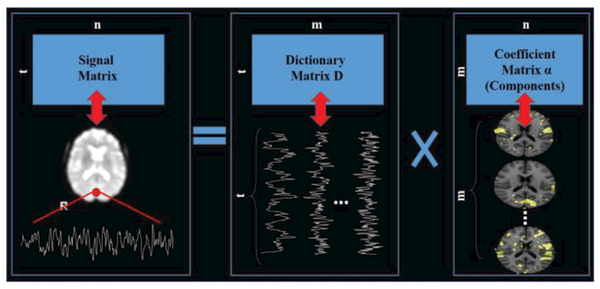
After preprocessing, dictionary learning and sparse coding techniques were exploited for functional brain networks reconstruction, as summarized in Fig. 1. The input for dictionary learning is a matrix $X\in {\Re }^{t\times n}$ with t (number of time points rows and n columns containing normalized fMRI signals from n brain voxels of an individual subject. The output contains one learned dictionary D and a sparse coefficient matrix $\alpha \in {\Re }^{m\times n}$, w.r.t, X =D × α + ε, where ε is the error term and m is the predefined dictionary size. Each row of the output coefficient matrix α was then mapped back to the brain volume space as a spatial map of functional brain network. According to [6], dictionary size was empirically set to for a comprehensive functional brain networks reconstruction. Each subject with 7 task-based and 1 resting-state fMRI data is labelled using 10 RSN templates, making the total number of RSNs for 68 subjects 68*80=5440. Since some subjects have missing task-based fMRI data or fMRI-derived brain networks, the final number of the RSNs is 5275. The labeling process using 2D image visualization is shown in Supplemental Fig. 1. Even though the use of the 2D image visualization will compromise the 3D pattern distribution in the manual distribution, using 48 informative slices 2D image is still more intuitive and faster than using the 3D overlap images. The reason is that experts need to examine the overlap information of the input map and the templates respectively, and generating the 3D images needs fine threshold tuning and would cost a huge amount of time for the whole labeling process (Supplemental Fig. 2). More importantly, our results showed that the mislabeled maps will be corrected by the proposed CNN structure. Thus 3D overlap visualization is only used when comparing the CNN prediction discrepancies with the original labels. All of the RSNs (5275 in total in the HCP Q1 dataset with manual labels of 1 RSNs are visualized at (http://hafni.cs.uga.edu/finalizednetworks_Resting.html. Due to the spatial resolution of 2mm, the initial voxel dimension of one volume map is 91×109×91.In order to reduce computational burden, all of the functional RNSs maps were down sampled from the resolution of 91×109×91 to 45×54×45.

Fig. 1.

Functional brain networks reconstruction using dictionary learning and sparse representation of whole-brain fMRI signals. Each row of the coefficient matrix α is mapped back to the volume space as a spatial map for carrying out the the classification task.

B. Computational Frameworks

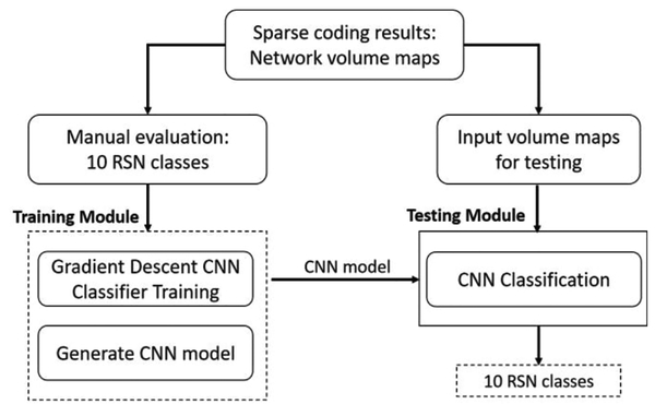
An fMRI oriented 3D CNN structure was designed for the problem of RSNs identification and recognition. The overall computational framework contains the two key steps, CNN training and testing (Fig. 2). Both training set and testing set were selected among the 5070 manually labelled RSNs. Specifically,80% of the labelled data were randomly selected as the training set, while the remaining 20% were treated as the testing set. Detailed information of the training and testing RSNs is summarized in Table 1. In particular, balanced amount of dataset of each label for the training set was maintained to achieve a balanced training performance for each label [34].

Fig. 2.

Overview of the computational steps in the 3D CNN framework. All the obtained maps from Fig. 1 are evaluated manually with 10 RSN labels. Then the whole dataset is divided into a training set and testing set. Training module uses the training set to train the weights of the constructed CNN structure and then is applied to the testing set the get the predicted labels.

Table I.

RSNS NUMBERS OF TRAINING SETS AND TESTING SETS FOR 3D CNN TRAINING AND TESTING.

	RSN1	RSN2	RSN3	RSN4	RSN5	RSN6	RSN7	RSN8	RSN9	RSN10	total
Training	377	373	380	361	384	380	354	373	382	390	3754
Testing	149	154	146	176	146	140	175	155	141	139	1521

C. 3D CNN Structure

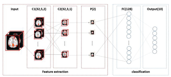
Prior studies have shown that a hierarchy of useful features can be learnt from CNN deep learning models. Such learning models can be trained with either supervised or unsupervised approaches. However, many previous CNN-related researches are 2D-centric [35], which might not be optimal for 3D volumetric image representation and could potentially overlook 3D structure information like in our application scenario of 3D RSNs recognition. In this work, we adopt and improve an effective fully 3D CNN framework [31] to train convolutional neural networks that aim to classify and recognize RSNs reconstructed by dictionary learning and sparse coding methods. This powerful 3D convolutional architecture can well incorporate 3D structure information as intrinsic features, and effectively model the variability of the RSNs volume maps for classification and recognition, as demonstrated in the result section. Besides, the deep-layered nature of CNNs can effectively extract more abstract feature representation of the input RSN maps with deeper layers. These promising characteristics of 3D CNN make it suitable and ideal for automatic, effective and accurate classification and recognition of these large numbers of FMRI derived functional brain networks. The proposed 3D CNN structure is summarized in Fig. 3. The detailed information of each layer and training procedure will be explained in the following sections, respectively.

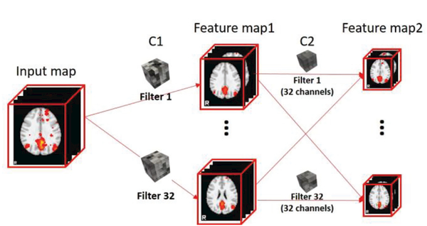
Fig. 3.

Overview of the 3D CNN structure. Input map and output of each feature extraction layer are visualized. C1 represents convolutional layer 1, which contains 32 types of kernels or filters of size Ȉ with a stride step 2; C2 represents convolutional layer 2, which contains 32 types of kernels of filters of size 3 with a stride step 2;C2 represents pooling layer with pooling kernel size of 2; FC represents fully connected layer, with 128 nodes in this layer; Output layer contains 10 nodes representing each class of the 10 RSNs labels.

Convolutional layers:

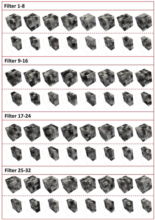
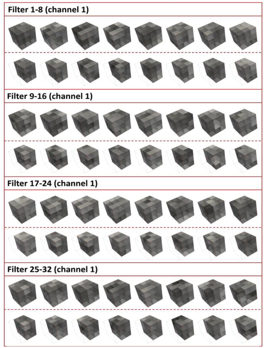
The convolutional layer of the CNN structure is denoted as C(f,d,s), where f is the number of filters or kernels, also the number of feature maps after filtering; d is the size of the 3D filter; s is the stride step. (ach convolutional layer is followed by a leaky rectified nonlinearity unit (ReLU) [36] with parameter 0.1, which is not shown in Fig. 3. for brevity. The initialization scheme of the convolutional layers was adopted from the methods in [27]. After the training stage, RSNs specific filters were obtained for all the convolutional layers, as shown in Fig. 4 and Fig. 5 for the purpose of visualization of filters in convolutional layer 1 and 2.

Fig. 4.

Visualization of the trained RSNs-specific filters for convolutional layer 1. This layer contains 32 different types of filters, each of which has a size of 5*5*5*32, with entire filters and clipped filters separated by a dashed line in the middle of each panel.

Fig. 5.

Visualization of the trained RSNs-specific filters for convolutional layer 2. This layer also contains 32 different types of filters, each of which has a size of 3*3*3*32 (32 input channels for this layers). Here, only the filters for the first channel of all the 32 are shown, with entire filters and clipped filters separated by a dashed line in the middle in each panel.

Notably, the input RSNs can be well represented using feature maps obtained by convolving with the well -trained filters. To demonstrate this point, an example of a default mode network (DMN) [37] as input is shown in Fig. 6 to illustrated the powerful feature extraction ability of the proposed 2 layered convolutional structure. Typically, DMN has 6 meaningful regions of interests (ROIs , which can be well captured through different perspectives after convolutional layers (due to limited number of slices selected for visualization, only 4 ROIs are displayed in feature map1 and feature map2 in Fig. 6), as shown in Fig. 6.

Fig. 6.

Extracted feature maps using trained CNN layers with DMN as an input example.

Pooling layer:

A pooling layer is connected to down sample the convoluted feature maps. This layer reduces the size of the input for the following classification layers, which substantially reduces redundant input information. Also, due to the translation-invariance properties of the pooling layer [38], the global shift resulted by preprocessing steps (such as image registration) and the intrinsic shape and size variability of RSNs from different brains can be significantly alleviated and accounted for. This is one of the major advantages of using 3D CNN for automatic and robust recognition of RSNs, compared to other methods reviewed in the introduction section. In this paper, a max pooling scheme with pooling size of 2 was adopted and it turned out to work well.

Fully connected layer and output layer:

These two layers are functioning as the classification/recognition component in the overall 3D CNN framework. With well-extracted features as input, 128 nodes of the fully connected layer can effectively perform the classification task. The output layer contains 10 nodes, each of which predicts the corresponding RSN label probability for each input map by adopting the SoftMax action function. CNN training: The neural network weights training was performed by the classic Stochastic Gradient Descent (SGD with momentum. The objective loss function to be optimized is the multinomial negative log-likelihood with a λ (set to 0.01) times the L2 norm of the network weights as regularization term, as shown in equation (1).

$$L(\theta )=-\frac{1}{m}{\displaystyle \sum }_{i=1}^m{\displaystyle \sum }_{j=1}^{k}1·\left\{y^i=j\right\}\log {\left({\theta }^T{x}^i\right)}_j+\lambda {\Vert \theta \Vert }_2$$ (1)

where m is the number of samples in one batch (empirically set to 32), and K is the number of the output classes (10 output RSN classes) and $\log {({\theta }^T{x}^i)}_j$ is the log-likelihood activation value of the j_th output node.The momentum parameter was set to 0.9. In this work, the widely-used dropout technique was adopted for each layer during the training process to reduce the overfitting problem that may be caused by large amount of weights to be trained and to reduce testing errors [22], [39].The convolutional layers were initialized using the similar scheme proposed in [27], and the dense layers were initialized with a Gaussian distribution with μ=0, σ = 0.01.Training was performed by utilizing GPU (NVidia Quadro M4000 8GB memory) for 80 epoches.During training, we choose the batch size to be 2048, and each training instance is a 47*56*47 3D volume. So the data usage is 0.94GB as the 32 bits float type, and the total usage of GPU memory during training is 1.17GB. For all the 3754 training RSNs samples, the total training time is less than 20 minutes. This scale of training time cost makes the proposed 3D CNN framework very suitable for future cognitive and clinical neuroscience applications.

III. Results

In this section, a variety of experiments and comparisons are conducted to evaluate the performance of the proposed 3D CNN framework. Traditional automated RSN identification method using overlap rate was performed in comparison to our proposed RSN identification framework using CNN structure. This overlap rate based method is very intuitive by using the calculated overlap rates between input network and RSN templates as the similarity metric. The overlap rate is calculated according to equation (2).

$$overlaprate={\displaystyle \sum _{K=1}^{\left|V\right|}\frac{\min (V_{k,}{W}_k)}{(V_k+W_K)/2}}$$ (2)

where V_K and W_k are the activation score of voxel k in RSN volume maps V and W, respectively. According to [14], row of the dictionary learning and sparse coding α matrix represents the spatial volumetric distributions that have references to certain dictionary atoms. Spatial activation score at each voxel is the normalized coefficient in the corresponding column of α matrix after dictionary learning and sparse coding. After pairwise overlap rate calculation between each RSN and the 10 templates, the template with the maximum overlap rate to the RSN was assignest with the template’s label to the RSN. Two additional widely-used classifiers, including the logistic regression and multi-class linear support vector machine (SVM), are also used for comparisons.

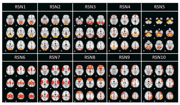
For 1521 testing RSN samples, based on the originally manually labelled RSNs, 94.61% accuracy was achieved by using the proposed 3D CNN framework. In contrast, only ˙85.93% accuracy was achieved by overlap rate, and 91.98% and 91.78% accuracies were achieved by the logistic regression and multi-class SVM respectively, which are all outperformed by our CNN classifier. Since spatial overlap rate is a widely-used way to evaluate the spatial maps, in the following discussion, we only compare the spatial overlap rate method with our proposed CNN methods. Among the 5.39% CNN-based error rate (82 testing errors) and 14.07% overlap-based error rate (214 testing errors), there were 4.4% (67 testing case errors) in common. Overall, CNN classification results significantly outperformed overlap-based results by round 10%. The promising results indicated the powerful spatial description ability of CNN. Through the detailed analysis and visualization of CNN classification error patterns in the following sub-sessions, we will further demonstrate that our designed CNN framework has the ability of accommodating major distributions of the training samples and ignoring outliers in the training samples, thus correcting the wrongly labelled RSNs due to the manual labelling mistakes. For the rest of the sub-sections, the 10 common RSNs templates derived from our HAFNI project [14] are visualized in Fig. 7 and will be used as a common spatial reference for evaluations and comparisons.

Fig. 7.

Visualization of 10 common RSNs templates derived in the HAFNI project. For each RSN, 9 most informative slices are displayed.

A. Correction of Wrongly Manually-Labeled RSNs by 3D CNN

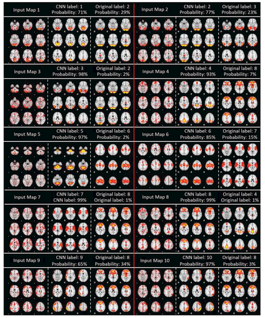
Among a large portion of CNN-based RSN classification errors (82 in total), there are actually testing cases that were originally wrongly labeled by experts. For each of these 10 RSNs we selected one representative example of CNN classification error for visualization in Fig. 8 to demonstrate the CNN’s ability of manual label correction. In this case, the real meaning of “wrong” CNN classification is that its prediction does not agree with the expert’s manual labeling. Therefore, if this scenario is double-checked and confirmed, CNN’s prediction can be used to correct the originally wrongly labeled RSNs by expert. As shown in Fig. 8, CNN classified labels appear to be more reasonable than the original manual labels, which has been confirmed by separate senior experts other than the original experts. In addition, quantitative measurement of the probability (the softmax values of the output layer of correct labeling by both CNN and original manual labeling is provided for each representative case on the top of each figure panel in Fig. 8. Among all the 82 testing cases with CNN’s “wrong” classifications, 63 of them are considered as CNN’s corrections of original wrongly-labeled RSNs (see Table 2. for detailed numbers for each of 10 RSN types), while still 15 of them are remained controversial. For the visualizations of all of 82 CNN prediction errors, please refer to http://hafni.cs.uga.edu//CNNClassification/errorCheckCNNerrorAll/index1.html.

Fig. 8.

Representative cases of CNN classification errors for 10 RSNs. CNN’s predicted labels (denoted as CNN label in the figure) appear to be more reasonable than the original manual labels by experts. Each panel has 3 columns, where the 1^st column is the input map, the 2^nd column is the RSN template with the CNN predicted label, and the 3^rd column is the RSN template with the original label. CNN probability is the output value of the softmax representing the confidence of the predictions.

Table II.

CNN corrections of original wrong labels for each of the 10 RSN types.

	RSN1	RSN2	RSN3	RSN4	RSN5	RSN6	RSN7	RSN8	RSN9	RSN10	total
Wrongly labelled	2	3	9	30	5	6	3	7	1	0	63

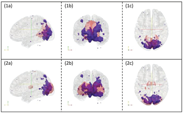
It is noted that the original expert manual labelling of 10 RSNs was based on 2D visualization of RSNs’ volume slices as shown in Fig. 8. In this study, to double-check and confirm the CNN’s corrections of those wrongly manually-labelled RSNs, we conducted a more informative 3D visualization of those RSNs using input map 1 in Fig. 8 together with RSN 1 and RSN 2 as illustration examples, as shown in Fig. 9. It is evident that the CNN’s predicted labels truly to be more reasonable than the original manual labels.

Fig. 9.

3D visualizations of input map 1 in figure 8 with RSN templates overlaid. Subfigure (1a), (1b) and (1c) are input maps (blue regions) with RSN1 overlaid (red regions). They are displayed with cross sections along the x, y and z axes respectively. Subfigure (2a), (2b) and (2c) are input maps (blue regions) with RSN2 overlaid (red regions). They are displayed with cross sections along the x, y and z axes respectively.

B. Overlap-based Classification Error Analysis

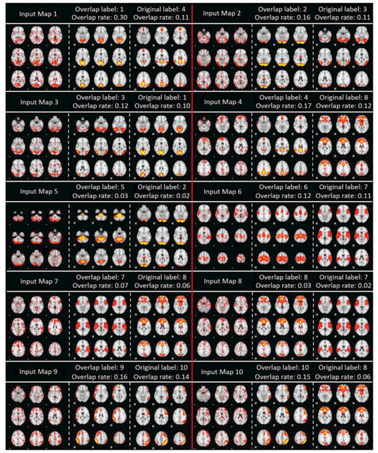
In comparison with 82 cases of CNN’s disagreements with original manual labels, overlap-based method has 214 disagreements with original manual labels. It turns out that overlap-based method shares common disagreements with original manual labels with the CNN method (to be detailed in section 3.3), and overlap-based method can be more reasonable than the original manual label in some cases. For example, in Fig. 1 , for RSN map 1, 3, 6, overlap-based prediction labels seem to be more reasonable. However, in many cases, manual labels are more reasonable. As shown in Fig. 1 , for RSN map 2, 3, , 1 , overlap-based method had made obviously less reasonable predictions. Among those 21 disagreements with original manual labels by overlap-based methods, ˙9 of them are believed to be truly wrong classification. In this sense, CNN method certainly significantly outperforms overlap-based method. All the visualizations of the 21 overlap-based predictions can be found on http://hafni.cs.uga.edu/CNNClassification/errorCheckOverlapAll/index1.html.

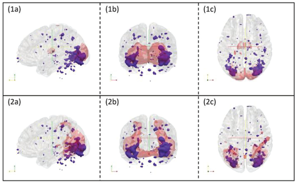
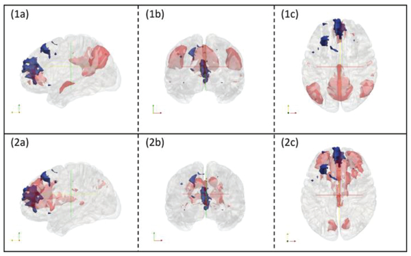
As examples, Fig. 11 confirms that for input map 2 in Fig. 10, overlap-based method really made wrong classification. This wrong classification might be caused by a variety of reasons, among which spatial registration, alignment error and noise sources could be a major issue; Fig. 12 confirms that for input map 4 in Fig. 10, overlap-based method made unreasonable classification. This type of wrong classification is due to the intrinsic heterogeneous activities of intermixed neurons in the same brain region or voxel [40].

Fig. 11.

3D visualizations of input map 2 in figure 10 with RSN templates overlaid. Subfigure (1a), (1b) and (1c) are input maps (blue regions) with overlap-based classification of RSN2 template overlaid (red regions). They are displayed with cross sections along the x, y and z axes respectively. Subfigure (2a), (2b) and (2c) are input maps (blue regions) with RSN3 overlaid (red regions). They are displayed with cross sections along the x, y and z axes respectively. RSN3 should be the category for this input map, but overlap-based method gave the wrong result as RSN2.

Fig. 10.

Representative cases of overlap-based classification results for 10 RSNs. Each panel has 3 columns, where the 1^st column is the input map, the 2^nd column is the RSN template with the overlap rate predicted label, and the 3^rd column is the RSN template with the original label. Overlap rate value calculated using equation (2) with the templates are shown correspondingly.

Fig. 12.

3D visualizations of input map 4 in figure 10 with RSN templates overlaid. Subfigure (1a), (1b) and (1c) are input maps (blue regions) with overlap-based classification of RSN template overlaid (red regions). They are displayed with cross sections along the x, y and z axes respectively. Subfigure (2a), (2b) and (2c) are input maps (blue regions) with RSN˙ overlaid (red regions). They are displayed with cross sections along the x, y and z axes respectively. Due to that the major activation regions reside in the prefrontal lobes, RSN˙ should be the category for this input map, but overlap-based method gave the wrong result.

C. Common Disagreements with Manual Labels by CNN and Overlap-based Method

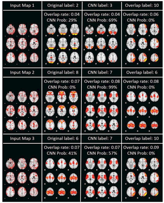
Our experiment results show that CNN and overlap-based method share 67 common disagreements with the original manual labels. Interestingly, all of these 67 RSN maps tend to be manually assigned with wrong labels. Among the 67 classifications, 64 of them were predicted with the same label using both CNN and overlap-based method. However, there are other 3 RSNs that have different annotations from manual labelling, CNN and overlap-based method, and these 3 RSNs and their different labels by three methods are visualized in Fig. 13. As we can see, among the 3 CNN labels, the RSN map 2 has the highest CNN prediction probability (99%), while the other two RSN maps have relatively low probabilities. From visual inspections, we really cannot tell which classes the input RSN map 1 and 3 should belong to. This problem might be caused by the relative low quality of the input RSN maps. Nevertheless, it is certain that input RSN map 2 should be assigned with label 7, which means the high prediction probability provided by CNN is quite reliable. For all the 67 common disagreements with the original manual labels, please refer to http://hafni.cs.uga.eduCNNClassification/errorCommon/index1.html

Fig. 13.

3 RSN classification discrepancies between CNN and overlap-based method in common prediction disagreement with the original manual labels. Each instance is shown using an entire row with 4 columns, with one input map, the RSN template of original label, CNN label and overlap label.

D. Differentiation between Highly Spatially Overlapped RSNs

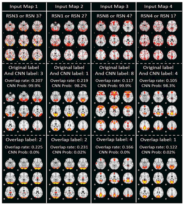
fMRI signal from each voxel reflects a highly heterogeneous mixture of functional activities of the entire neuronal assembly of multiple cell types in a voxel. In addition to the heterogeneity of neuronal activities, the convergent and divergent axonal projections in the brain and heterogeneous activities of intermixed neurons in the same brain region or voxel demonstrate that cortical microcircuits are not independent and segregated in space, but they rather overlap and interdigitate with each other [40]. Thus spatial overlap of functional networks including RSNs is a natural property of functional organization of the human brain [41]. In this paper, among the 10 RSNs specifically, template RSN2 and RSN3, RSN1 and RSN2, RSN4 and RSN8, RSN1 and RSN4 have relative high spatial overlap rates (0.1665, 0.1550, 0.1201 and 0.1062, respectively), which made the overlap-based method difficult to differentiate those pairs of highly overlapping RSN patterns. Four examples of such cases have been shown in Fig. 14 to demonstrate the advantages of CNN over overlap-based method when differentiating highly overlapped spatial patterns. More such examples can be found on the webpage showing CNN’s only disagreements with manual labels (http://hafni.cs.uga.edu/CNNClassification/errorCheckOnlyCNN/index1.html) and overlap-based only method’s disagreements with manual labels (http://hafni.cs.uga.edu/CNNClassification/errorCheckOnlyOverlap/index1.html)

Fig. 14.

Illustration of CNN and overlap-based method’s performance when differentiating input RSN maps of high spatial overlaps. Each column represents one instance with 3 rows: the input map, the RSN template with the CNN label and the overlap label. As shown by each instance, all the input maps have relatively high overlap rate with both of the templates (>=0.10), making the overlap rate hard to predict correctly. However, CNN makes the correct prediction regardless of the high overlap rates.

IV. Discussion and conclusion

The HAFNI framework has enabled connectome-scale reconstruction of reproducible and meaningful functional brain networks on large-scale populations such as the HCP datasets. However, an unsolved problem in the HAFNI framework is the automatic recognition of HAFNI maps such as RSNs in each individual brain. The major problem in previous methods is that they are not able to deal with the tremendous variability of various types of functional brain networks (e.g. size, shape and location) and the presence of various sources of noises. In this study, we have proposed and applied a fully automatic 3D CNN deep learning framework to identify and classify different types of functional brain networks with promising performance. Our experimental results showed a promising classification accuracy of 94.61% by improving approximately 10% compared to overlap-based method. Furthermore, in the result subsections, we conducted comprehensive analysis of the disagreement patterns of CNN labels with manual labels, as well as the overlap-based method’s labels. Our results demonstrated the superior performance of CNN in recognizing ambiguous RSNs, spatially overlapping RSNs, and misaligned RSNs. In general, our work provides a new deep learning approach for modeling functional connectomes based on FMRI data, particularly fMRI big data in the future.

Despite the great promise of the proposed CNN framework, however, there also exist challenges and limitations for the current CNN framework. First, the training sample preparation is a difficult issue for training the CNN networks. As we can see, manually labelled RSNs derived from our previous HAFNI project were used in this study, which entailed huge amount of time devoted to manually labeling dozens of thousands of functional network maps, among which thousands of them are RSNs. Also, manual labeling mistakes and inter-rater variability of labels are inevitable. Though our CNN framework already exhibits the promising property of correcting wrongly manually labeled RSNs, as shown in the result sections, a reliable and fully or semi- automated network labelling method should be explored in the near future to enlarge the training samples and improve the training accuracy. Also, since the correction ability is supported by the training set distribution modelling process and the outliers or the wrongly labelled data are still a minority, we plan to investigate what is the maximally allowed outlier portion in the training set in the future. Second, the problem of 10 RSN classifications was employed in this study for experiment setup, which was just a testbed and showcase for the efficiency of our CNN framework. In the future, we will develop and use larger scale training sample generation and build a CNN model for classifications and recognitions of many more types of functional networks such as hundreds of networks that were already revealed in our HAFNI project. Third, other advanced or sophisticated CNN structures, e.g., multi scale CNN [42] or truly deep CNN [23], [28], [43], will be explored in the near future. It is expected that these improved CNN structures will possess better ability of spatially representing 3D networks maps and thus will further generate better network classification results. Finally, we plan to adopt and apply these effective CNN frameworks on clinical fMRI datasets for the better understanding of altered brain networks in brain diseases such as Alzheimer’s disease and Autism. We envision that 3D CNN model will significantly advance current state-of-the-art fMRI data modeling approaches and pave the way for adopting fMRI into clinical management of brain disorders in the future.

REFERENCES

- [1].McKeown MJ et al. , “Analysis of fMRI data by blind separation into independent spatial components,” Hum. Brain Mapp, vol. 6, no. 3, pp. 16–188, Jan. 1998. [DOI] [PMC free article] [PubMed] [Google Scholar]
- [2].Beckmann CF and Smith SM, “Probabilistic independent component analysis for functional magnetic resonance imaging.,” IEEE Trans. Med. Imaging, vol. 23, no. 2, pp. 137–52, Feb. 2004. [DOI] [PubMed] [Google Scholar]
- [3].Rolfe SM et al. , “An independent component analysis based tool for exploring functional connections in the brain,” 2009, p. 725921. [Google Scholar]
- [4].De Martino F et al. , “Classification of fMRI independent components using IC-fingerprints and support vector machine classifiers,” Neuroimage, vol. 3 , no. 1, pp. 177–194, 2007. [DOI] [PubMed] [Google Scholar]
- [5].McKeown MJ, Hansen LK, and Sejnowsk TJ, “Independent component analysis of functional MRI: what is signal and what is noise?,” Curr. Opin. Neurobiol, vol. 13, no. 5, pp. 620–629, 2003. [DOI] [PMC free article] [PubMed] [Google Scholar]
- [6].Lv J et al. , “Sparse representation of whole-brain fMRI signals for identification of functional networks.,” Med. Image Anal, vol. 2 , no. 1, pp. 112–34, Feb. 2015. [DOI] [PubMed] [Google Scholar]
- [7].Lv J et al. , “Identifying functional networks via sparse coding of whole brain FMRI signals,” in 2013. 6th International IEEE/EMBS Conference on Neural Engineering (NER), 2 13, pp.788–781. [Google Scholar]
- [8].Lv J et al. , “Modeling Task FMRI Data via Supervised Stochastic Coordinate Coding,” Springer International Publishing, 2015, pp. 239–246. [Google Scholar]
- [9].Jiang X et al. , “Sparse representation of HC P grayordinate data reveals novel functional architecture of cerebral cortex,” Hum. Brain Mapp, vol. 36, no. 12, pp. 5301–5319, Dec. 2015. [DOI] [PMC free article] [PubMed] [Google Scholar]
- [10].Zhao S et al. , “Supervised Dictionary Learning for Inferring Concurrent Brain Networks,” IEEE Trans. Med. Imaging, vol. 34, no. 10, pp. 2036–2045, Oct. 2015. [DOI] [PubMed] [Google Scholar]
- [11].Lv J et al. , “Assessing effects of prenatal alcohol exposure using group wise sparse representation of fMRI data.,” Psychiatry Res, vol. 233, no. 2, pp. 254–68, Aug. 2015. [DOI] [PMC free article] [PubMed] [Google Scholar]
- [12].Zhang S, Li X, Lv J, Jiang X, Guo L, and Liu T, “Characterizing and differentiating task based and resting state fMRI signals via two-stage sparse representations,” Brain Imaging Behav, vol. 10, no. 1, pp. 21–32, Mar. 2016. [DOI] [PMC free article] [PubMed] [Google Scholar]
- [13].Mairal J, Bach F, Ponce J, and Sapiro G, “Online Learning for Matrix Factorization and Sparse Coding,” J. Mach. Learn. Res, vol. 11, pp. 19–60, Mar. 2010. [Google Scholar]
- [14].Lv J et al. , “Holistic atlases of functional networks and interactions reveal reciprocal organizational architecture of cortical function.,” IEEE Trans. Biomed. Eng, vol. 62, no.4, pp. 1120–31, Apr. 2015. [DOI] [PubMed] [Google Scholar]
- [15].Zhao Y et al. , “Connectome-scale group-wise consistent resting-state network analysis in autism spectrum disorder.,” NeuroImage. Clin, vol. 12, pp. 23–33, 2016. [DOI] [PMC free article] [PubMed] [Google Scholar]
- [16].Kennedy DP and Courchesne E, “Functional abnormalities of the default network during self- and other reflection in autism.,” Soc. Cogn. Affect. Neurosci, vol. 3, no. 2, pp. 177–90, Jun. 2008. [DOI] [PMC free article] [PubMed] [Google Scholar]
- [17].Zhu D et al. , “Connectome-scale assessments of structural and functional connectivity in MCI.,” Hum. Brain Mapp, vol. 35, no.7, pp. 2911–23, Jul. 2014. [DOI] [PMC free article] [PubMed] [Google Scholar]
- [18].Wang Y and Li T-Q, “Dimensionality of ICA in resting state fMRI investigated by feature optimized classification of independent components with SVM.,” Front. Hum. Neurosci, vol. 9, p. 259, 2015. [DOI] [PMC free article] [PubMed] [Google Scholar]
- [19].Bartels A and Zeki S, “Brain dynamics during natural viewing conditions—A new guide for mapping connectivity in vivo,” Neuroimage, vol. 2 , no. 2, pp. 339–349, 2005. [DOI] [PubMed] [Google Scholar]
- [20].Perlbarg V, Bellec P, Anton J-L, Pélégrini-Issac M, Doyon J, and Benali H, “CORSICA: correction of structured noise in fMRI by automatic identification of ICA components.,” Magn. Reson. Imaging, vol. 25, no. 1, pp. 35–46, Jan. 2007. [DOI] [PubMed] [Google Scholar]
- [21].Lecun Y, Eon Bottou L, Bengio Y, and Haaner P, “Gradient-Based Learning Applied to Document Recognition RS S90 Reduced set support vector method. SDNN Space displacement neural network. SVM Support vector method. TDNN Time delay neural network. V - SVM Virtual support vector method,” PROC. IEEE, 1998. [Google Scholar]
- [22].Krizhevsky A, Sutskever I, and Hinton GE, “ImageNet Classification with Deep Convolutional Neural Networks,” in NIPS, 2012, pp. 1097–1105. [Google Scholar]
- [23].Simonyan K and Zisserman A, “Very Deep Convolutional Networks for Large-Scale Image Recognition,” Sep. 2014. [Google Scholar]
- [24].Lawrence S, Giles CL, Tsoi Ah Chung, and Back AD, “Face recognition: a convolutional neural-network approach,” IEEE Trans. Neural Networks, vol. 8, no. 1, pp. 98–113, 1997. [DOI] [PubMed] [Google Scholar]
- [25].Karpathy A, Toderici G, Shetty S, Leung T, Sukthankar R, and Fei Fei L, “Large-scale Video Classification with Convolutional Neural Networks,” 2014, pp. 1725–1732. [Google Scholar]
- [26].Liu Nian, Han J, Zhang D, Wen Shifeng, and Liu T, “Predicting eye fixations using convolutional neural networks,” in 2015 IEEE Conference on Computer Vision and Pattern Recognition (CVPR), 2015, pp. 362–370. [Google Scholar]
- [27].He K, Zhang X, Ren S, and Sun J, “Delving Deep into Rectifiers: Surpassing Human Level Performance on ImageNet Classification,” Feb. 2015. [Google Scholar]
- [28].He K, Zhang X, Ren S, and Sun J, “Deep Residual Learning for Image Recognition,” Dec. 2015. [Google Scholar]
- [29].Ji S, Xu W, Yang M, and Yu K, “3D Convolutional Neural Networks for Human Action Recognition,” IEEE Trans. Pattern Anal. Mach. Intell, vol. 35, no. 1, pp. 221–231, Jan. 2013. [DOI] [PubMed] [Google Scholar]
- [30].Li R et al. , “Deep learning based imaging data completion for improved brain disease diagnosis.,” Med. Image Comput. Comput. Assist. Interv, vol. 17, no. Pt 3, pp. 305–12, 2014. [DOI] [PMC free article] [PubMed] [Google Scholar]
- [31].Maturana D and Scherer S, “VoxNet: A 3D Convolutional Neural Network for real time object recognition,” in 2015 IEEE/RSJ International Conference on Intelligent Robots and Systems (IROS), 2015, pp. 922–928. [Google Scholar]
- [32].March DM et al. , “Function in the human connectome: task fMRI and individual differences in behavior.,” Neuroimage, vol. 80, pp. 169–89, Oct. 2013. [DOI] [PMC free article] [PubMed] [Google Scholar]
- [33].Smith SM et al. , “Resting-state fMRI in the Human Connectome Project,” Neuroimage, vol. 80, pp. 144–168, 2013. [DOI] [PMC free article] [PubMed] [Google Scholar]
- [34].Mazurowski MA, Habas PA, Zurada JM, Lo JY, Baker JA, and Tourassi GD, “Training neural network classifiers for medical decision making: the effects of imbalanced datasets on classification performance.,” Neural Netw, vol. 21, no. 2–3, pp. 427–36, 2008 [DOI] [PMC free article] [PubMed] [Google Scholar]
- [35].Gupta S, Girshick R, Arbeláez P, and Malik J, “Learning Rich Features from RGB-D Images for Object Detection and Segmentation,” Jul. 2014.
- [36].Maas AL, Hannun AY, and Ng AY, “Rectifier Nonlinearities Improve Neural Network Acoustic Models,” ICML, 2013. [Google Scholar]
- [37].Smith SM et al. , “Correspondence of the brain’s functional architecture during activation and rest.,” Proc. Natl. Acad. Sci. U. S. A, vol. 106, no. 31, pp. 13040–5, Aug. 2009. [DOI] [PMC free article] [PubMed] [Google Scholar]
- [38].Scherer D, Müller A, and Behnke S, “Evaluation of Pooling Operations in Convolutional Architectures for Object Recognition,” Springer Berlin Heidelberg, 2010, pp. 92–101. [Google Scholar]
- [39].Bell RM and Koren Y, “Lessons from the Netflix prize challenge,” ACM SIGKDD Explor. Newsl, vol. 9, no. 2, p. 75, Dec. 2007. [Google Scholar]
- [40].Harris KD and Mrsic Flogel TD, “Cortical connectivity and sensory coding,” Nature, vol. 503, no. 7474, pp. 51–58, Nov. 2013. [DOI] [PubMed] [Google Scholar]
- [41].Xu J et al. , “Large-scale functional network overlap is a general property of brain functional organization: Reconciling inconsistent fMRI findings from general-linear-model-based analyses,” Neurosci. Biobehav. Rev, vol. 71, pp. 83–100, 2016. [DOI] [PMC free article] [PubMed] [Google Scholar]
- [42].Nian Liu XL, Han Junwei, Liu Tianming, “Learning to Predict Eye Fixations via Multiresolution Convolutional Neural Networks,” IEEE Trans. Neural Networks Learn. Syst, vol. Accepted, 2016. [DOI] [PubMed] [Google Scholar]
- [43].Szegedy C et al. , “Going Deeper With Convolutions,” in The IEEE Conference on Computer Vision and Pattern Recognition (CVPR), 2015, pp. 1–9. [Google Scholar]
Associated Data
This section collects any data citations, data availability statements, or supplementary materials included in this article.