A quantitative performance study of two automatic methods for the diagnosis of ovarian cancer

Highlights

• •We tackle the problem of early detection of ovariance cancer using longitudinal measurements of multiple biomarkers.
• •We compare two different paradigms: Bayesian methods and deep learning.
• •We provide evidence that using multiple biomarkers yields a performance boost as compared to the standard screening test using CA125 alone.

Abstract

We present a quantitative study of the performance of two automatic methods for the early detection of ovarian cancer that can exploit longitudinal measurements of multiple biomarkers. The study is carried out for a subset of the data collected in the UK Collaborative Trial of Ovarian Cancer Screening (UKCTOCS). We use statistical analysis techniques, such as the area under the Receiver Operating Characteristic (ROC) curve, for evaluating the performance of two techniques that aim at the classification of subjects as either healthy or suffering from the disease using time-series of multiple biomarkers as inputs. The first method relies on a Bayesian hierarchical model that establishes connections within a set of clinically interpretable parameters. The second technique is a purely discriminative method that employs a recurrent neural network (RNN) for the binary classification of the inputs. For the available dataset, the performance of the two detection schemes is similar (the area under ROC curve is 0.98 for the combination of three biomarkers) and the Bayesian approach has the advantage that its outputs (parameters estimates and their uncertainty) can be further analysed by a clinical expert.

1. Introduction

Ovarian cancer remains the fifth most common cause of cancer-related deaths among women, with more than 150,000 annual deceases worldwide. Most cases occur in post-menopausal women (75%), with an incidence of 40 per 100,000 per year in women aged over 50. The early detection of this disease increases 5-year survival significantly, from 3% in Stage IV to 90% in Stage I [1]. Therefore, it is important to design efficient methods for early detection.

The screening and initial procedures for the detection of ovarian cancer are often carried out by testing serum biomarkers that are known to correlate with the appearance of tumours. In particular, the serum biomarker Canger Antigen 125 (CA125) is the most commonly used oncomarker in the screening of ovarian cancer [2], [3], [4], [5]. However, other serum biomarkers have been reported to be associated with the development of ovarian cancer [6], [7], [8] and it has been recently suggested that they can be used in combination with CA125 [8], [9], [10], [11], [12], [13], [14]. The biomarker that has received more attention is the Human Epididymis Protein 4 (HE4), which has been used in the ROMA (Risk of Ovarian Malignancy Algorithm) to discriminate ovarian cancer from benign diseases [9], [15] as well as in different panels for the purpose of early detection [7], [10], [11]. In a study within the Prostate Lung Colorectal and Ovarian (PLCO) cancer screening trial [16], HE4 was the second best marker after CA125, with a sensitivity of 73% (95% confidence interval 0.60–0.86) compared to 86% (95% confidence interval 0.76–0.97) for CA125 [17], [18]. Another serum biomarker, glycodelin, has also shown promising performance in the detection of ovarian cancer [12], [19], [20].

Recently, time series data from multiple biomarkers, including CA125, HE4 and glycodelin, have been jointly analysed to determine whether the level of these markers changed significantly and coherently at specific time instants [6], associating this fact with the development of tumours. The focus in [6] was placed on the detection of change-points for different biomarkers, by estimating the probability of coincidences as well as the probability of the change-point of a given biomarker appearing (and being detected) earlier than others. As a consequence, it was suggested that the combined detection of change-points in several biomarkers could be exploited for early diagnosis of ovarian cancer. In this paper we address the quantitative study of this automatic diagnostic technique using statistical analysis tools.

In particular, we study the trade-off between sensitivity (proportion of correctly detected positives) and specificity (proportion of correctly detected negatives) of a detection procedure that relies on the Bayesian change-point (BCP) model described in [6] which, in turn, is a version of the model proposed originally in [21] for the ROCA (Risk of Ovarian Cancer Algorithm) scheme. The quantitative analysis is carried out for a subset of the data collected in the UK Collaborative Trial of Ovarian Cancer Screening (UKCTOCS) [22]. It involves time-series of CA125, HE4 and glycodelin for both healthy subjects (controls) and diagnosed patients (cases).

The decisions made by the BCP model involve estimating a number of parameters that admit a natural clinical interpretation. Although parsimony is always a desirable property to have in any model, accuracy (measured in terms of sensitivity and specificity) is here the ultimate goal. Hence, we also consider machine learning-based schemes which are often capable of modeling more complex mappings (between a set of measurements and the corresponding output) at the expense of some interpretability.

Deep learning (DL), and Recurrent Neural Networks (RNNs) in particular, have become important tools in classification tasks that involve the processing of ordered sequences of data [23]. Such methods have achieved state-of-the-art performance in applications such as handwriting [24], speech recognition [25] or image caption generation [26]. RNNS have also found many applications in the clinical field for tasks involving the classification of time series. In [27] a Long Short-Term Memory (LSTM) RNN is trained to classify diagnoses from pediatric intensive care unit (PICU) data. The same kind of data is fed to an RNN in [28] in order to predict mortality rates for patients in the intensive care unit. A Gate Recurrent Unit (GRU) is proposed in [29] for heart failure prediction. The authors of [30] use RNNs to assess the stress level of drivers from physiological signals coming from wearable sensors. In this work, we deploy a simple RNN for discriminating between women with ovarian cancer and healthy controls based on an ovarian cancer screening test that combines multiple biomarkers. The main challenge in applying DL in this context is the relatively small size of the dataset, which imposes some constraints on the kind of neural architectures that can be successfully trained without overfitting.

The ultimate goal in this paper is to carry out a comparison between these two different strategies (BCP and RNN) highlighting the advantages and disadvantages of both techniques. The study of both approaches, however, clearly shows that combining longitudinal time series of different biomarkers can improve the classification of pre-diagnosis samples regardless of the method.

The rest of this paper is organised as follows. Section 2 is devoted to the description of the dataset. Section 3 is devoted to a brief description of the Bayesian change-point method and the classification and statistical analysis carried out with it. In Section 4 the recurrent neural network technique is presented as well as the training procedure. The results obtained for both methods are presented and discussed in Section 5 and, finally, Section 6 is devoted to discussion and conclusions.

2. Data

The two methods have been applied to a dataset from the multimodal arm [6] of the UK Collaborative Trial of Ovarian Cancer Screening (UKCTOCS, number ISRCTN22488978; NCT00058032) [22], where women underwent annual screening tests using the blood tumour marker CA125. Biomarkers HE4 and glycodelin assays were additionally performed on stored serial samples from a subset of women in the multimodal arm diagnosed with ovarian cancer and controls. The dataset included 179 controls (healthy women) and 44 cases (diagnosed women): 35 cases of invasive epithelial ovarian cancer (iEOC), 3 cases of fallopian tube cancer and 6 cases of peritoneal cancer. Out of these 44 cases, 16 are early stage (International Federation of Ginecology and Obstetrics, FIGO [31], stages I and II) and 28 are late stage (FIGO stages III and IV). In terms of histology, there are 27 serous cancers, 2 papillary, 3 endometrioid, 2 clear cell, 3 carcinosarcoma, and 7 not specified cancers. Each control has 4 to 5 serial samples available (177 controls with 5 samples and 2 controls with 4 samples) and each case has 2 to 5 serial samples available (24 cases with 5 samples, 10 cases with 3 samples and 10 cases with 2 samples). For healthy women, the range of age is 50.3–78.8 years and the average age over all women and samples is 63.6 years. On the other hand, the range of ages for cases is 52.0–77.4 years and the average age over all women and samples is 65.5 years. A detailed classification of the women with cancer is shown in Table 1, indicating the range of ages and the average age of the different subgroups.

Table 1.

Classification of cases, showing the range of ages and the average age over the corresponding women and samples.

Histology	Stages	Number of women	Range of ages	Average age
Serous cancers	I–II	9	[52.0–69.0]	61.3
	III–IV	18	[54.9–76.7]	66.6
Papillary	I–II	1	[68.1–69.2]	68.6
	III–IV	1	[55.2–57.2]	56.2
Endometrioid	I–II	2	[60.3–64.3]	62.7
	III–IV	1	[67.6–68.7]	68.1
Clear cell	I–II	2	[57.0–77.4]	67.2
	III–IV	0	0	0
Carcinosarcoma	I–II	0	0	0
	III–IV	3	[60.0–67.2]	63.7
Not specified cancers	I–II	2	[72.7–74.2]	73.5
	III–IV	5	[62.5–73.0]	67.8

All serum samples were assayed for CA125, glycodelin and HE4 using a proprietary multiplexed immunoassay based on Luminex technology which was developed and run by Becton Dickinson.

It should be noted here that all the biomarker measurements have been modified via a logarithmic transformation, as detailed in [12], [21], in the form of Y = log(Z + 4), where Z is the value of a particular marker.

Traditionally, single-biomarker time-series have been employed for the screening of ovarian cancer patients, particularly CA125 data. Recently, a few studies [6], [12], [32], [33] have suggested that different biomarkers can be combined into multidimensional time-series and can lead to more accurate diagnosis. We explore this approach in the sequel.

3. Bayesian change-point method

3.1. Bayesian model

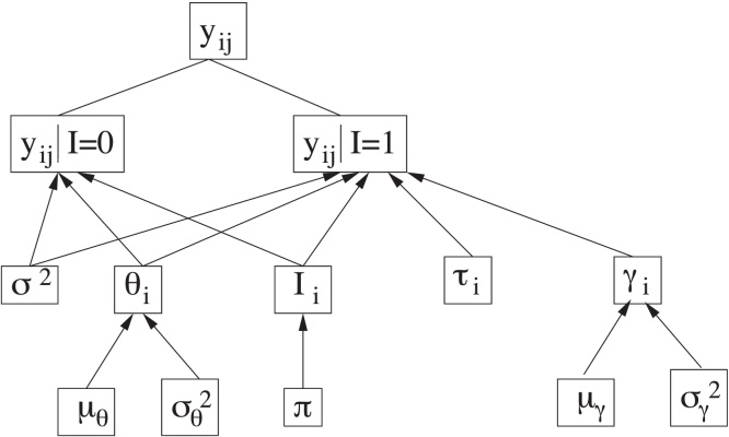
In order to analyse the available data, we adopt the Bayesian change-point model (BCP) described in [6], [21] and outlined in Fig. 1. Let y_ij denote the log-transformed measurement of the biomarker Z (where Z can be any of CA125, HE4 or glycodelin) for the ith woman in the study at age t_ij. The number of measurements for the ith subject is denoted k_i, so the time series consists of measurements collected at ages $t_{i1},\dots ,t_{{\mathrm{ik}}_i}$. The time t_ij of a measurement y_ij can depend on previous values $y_{{\mathrm{ij}}^{\prime }}$, j′ < j.

Fig. 1.

Scheme of the hierarchical Bayesian model.

Source: Fig. 1 from Ref. [6].

There are parameters in the model that are common to all women, namely those in the set $C=\{{\mu }_{\theta },{\mu }_{\gamma },{\sigma }_{\theta }^2,{\sigma }_{\gamma }^2,{\sigma }^2,\pi \}$, and parameters specific to each subject, namely S_i = {θ_i, I_i, τ_i, logγ_i}. A key parameter in the study to be carried out is the unobserved binary indicator I_i, which serves to determine whether the corresponding biomarker of the ith woman suffers or not a significative change in its behaviour. The indicator I_i for each woman is assumed to follow, a priori, a Bernoulli distribution with success probability π, where π represents the proportion of women for which we a priori expect a significant change in the time-evolution of the biomarker level, i.e., a change-point in the time series. We have chosen for the parameter π the prior distribution Beta(1.0, 1.0).

When the indicator of a given woman is I_i = 0 (expected for healthy women), all log-transformed measurements of this woman, y_ij (j = 1, …, k_i), are assumed to be modelled by a normal distribution with mean denoted E(y_ij|t_ij, I_i = 0) = θ_i and variance σ². This mean, θ_i, specific for each woman, is also assumed to follow a normal distribution with mean and variance denoted, respectively, as μ_θ and ${\sigma }_{\theta }^2$, common to all women. We have chosen the same prior distributions as in [6] for σ², μ_θ and ${\sigma }_{\theta }^2$. In particular, σ² ∼ IG(2.05, 0.1), ${\mu }_{\theta }\sim \mathcal{N}(2.75,1)$ and ${\sigma }_{\theta }^2\sim \mathrm{IG}(2.04,0.065)$, where $\mathcal{N}(a,b)$ denotes a normal distribution with mean a and variance b and IG(a, b) denotes the inverse gamma distribution with mean b/(a − 1) and variance b²/[(a − 1)²(a − 2)].

On the other hand, when the indicator of a given woman is I_i = 1 (expected for women with ovarian cancer), the corresponding measurements of this subject are assumed to be modelled by a normal distribution with mean represented by the piecewise linear function E(y_ij|t_ij, I_i = 1) = θ_i + γ_i(t_ij − τ_i)⁺ and variance σ² (the same as before). The notation (·)⁺ denotes the positive part of the expression between parentheses, γ_i represents the positive increase of the function that occurs after some time instant τ_i, referred as the change-point of the time series, and θ_i is modelled as explained above. As in [6], logγ_i is assumed to follow a normal distribution with mean and variance denoted, respectively, as μ_γ, ${\sigma }_{\gamma }^2$, common to all women. The same prior distributions as in [6] have also been chosen for μ_γ and ${\sigma }_{\gamma }^2$ and τ_i, namely ${\mu }_{\gamma }\sim \mathcal{N}(1.1,0.1)$, ${\sigma }_{\gamma }^2\sim \mathrm{IG}(2.2,0.12)$ and ${\tau }_i\sim \mathcal{T}\mathcal{N}(d_i-2,0.{75}^2,[d_i-5,d_i])$, where d_i denotes the age of patient i at the time of the last measurement and $\mathcal{T}\mathcal{N}(a,b,c)$ represents truncated normal distributions, with mean a, variance b and restricted to the interval c.

The posterior probability distributions for all unknown parameters of the model can be approximated using the Metropolis-within-Gibbs (MwG) sampling algorithm described in detail in [6]. This algorithm iteratively generates samples from the distribution of each parameter conditional on the current values of the other parameters. It can be shown that the resulting sequence of samples yields a Markov chain, and the stationary distribution of that Markov chain is the joint posterior probability distribution [34]. This is done with every biomarker, that is, CA125, HE4 and glycodelin.

3.2. Detection method

Unlike in [6], where the focus was placed on the change-point instant τ_i and its coherence across different biomarkers (i.e., whether the slope of different biomarkers series changed simultaneously or not), in this paper we propose to asses whether the ith subject has ovarian cancer or not based on the expected value of the indicator variable I_i given the available data.

Let m be the number of subjects in the dataset. In order to compute the expectation of I_i, i = 1, …, m, we run the MwG algorithm described in [6] to produce a chain of 10, 000 entries. Each entry of the chain contains one sample of each unknown parameter in the set $A={\bigcup }_{i=1}^m{S}_i\bigcup C$, which includes the common parameters in C and all subject-specific parameters. The first 5000 entries are removed (to ensure that the chain has converged) and the expected value of each I_i (i ∈ {1, …, m}) is estimated using the 5000 remaining entries in the chain, i.e., $E[I_i|\mathrm{data}]\approx \frac{1}{5000}{\sum }_{k=5000}^{10,000}{I}_i^{(k)}=:{\hat{I}}_i$, where $I_i^{(k)}$ is the kth sample of the ith indicator in the Markov chain. Detection can be carried out by comparing ${\hat{I}}_i$ to a threshold 0 < α < 1, in such a way that

• •if ${\hat{I}}_i<\alpha$ the ith subject is considered healthy, and a negative output is produced, and
• •if ${\hat{I}}_i>\alpha$ the disease is detected and a positive output is produced.

Some remarks are in order:

• •The detection threshold α can (and should) be optimised using the available data. In Section 5 we compute and plot the ROC curve that results from trying different values of α in the interval [0, 1] for the dataset described in Section 2. This curve can be used to select the value of α that yields suitable specificity (true negative rate) and sensitivity (true positive rate) values.
• •The BCP model and the estimator ${\hat{I}}_i$ can be used for “soft” detection. Intuitively, a value of ${\hat{I}}_i$ well above the selected α suggests a very confident positive (correspondingly, ${\hat{I}}_i<<\alpha$ points towards a clear negative), while a value of ${\hat{I}}_i$ close to α may trigger different tests or the inspection of that subject's data by an expert clinician.
• •The procedure can be naturally used on multiple biomarkers (and, indeed, we present such results in Section 5). When we compute the estimator ${\hat{I}}_i$ for several biomarkers we adopt the convention that the outcome is positive if ${\hat{I}}_i>\alpha$ for at least one biomarker, while it is negative if ${\hat{I}}_i<\alpha$ for all biomarkers. ROC curves (obtained by varying the threshold α) are displayed in Section 5 for the single-biomarker and multiple-biomarker cases.

4. Recurrent neural network

4.1. Network architecture

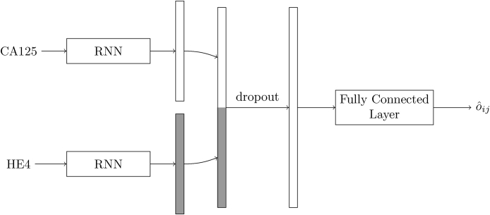
In a machine learning approach, we must decide whether a subject is healthy or not based on the value of (at most) three features, given by the measurements of the biomarkers (CA125, HE4, and glycodelin), and their corresponding time stamp. This is a small number of features and, when considering a deep learning approach, we should be careful to choose a network architecture that is simple enough as to avoid overfitting. With that in mind, we consider the most basic RNN followed by a dense layer, as shown in Fig. 2. For the ith subject, the input to the network is given by the sequence ${\text{x}}_{i1},{\text{x}}_{i2},\cdots ,{\text{x}}_{i{k}_i}$ where ${\text{x}}_{ij}={\left[t_{ij},y_{ij}\right]}^{\top }$ is a 2 × 1 column vector whose first element is the age of the subject, t_ij, and whose second element represents, as above, the log-transformed measurement of the biomarker Z (where Z can be any of CA125, HE4 or glycodelin) for the ith subject in the study at age t_ij. The hidden state of the network right before processing the jth input from the ith subject, x_ij, is given by the H × 1 (column) vector s_j−1, where H is the number of the hidden neurons. Then, the operation of the RNN is described by the equation

$${\text{s}}_j=f\left({\text{W}}_{\mathrm{ih}}{\text{x}}_{\mathrm{ij}}+{\text{b}}_{\mathrm{ih}}+{\text{W}}_{\mathrm{hh}}{\text{s}}_{j-1}\right)$$ (1)

where W_ih is the H × 2 input-hidden projection matrix, W_hh is the hidden layer (recurrent) kernel matrix of size H × H, b_ih is a H × 1 bias vector, and f(·) is an (element-wise) activation function. The latter is here the hyperbolic tangent, though other (usually non-linear) functions such as a Rectified Linear Unit (ReLU) or sigmoid function are also possible [23]. When the last sample for the ith subject, ${\text{x}}_{{\mathrm{ik}}_i}$, is fed to the RNN, the final output of the network for that subject is computed as

$${\hat{o}}_{{\mathrm{ik}}_i}=\sigma \left({\text{w}}_{\mathrm{ho}}^{\top }{\tilde{\text{s}}}_{k_i}+b_{\mathrm{ho}}\right)$$ (2)

where $\sigma (x)=1/\left(1+e^{-x}\right)$ is the sigmoid function, w_ho is the H × 1 hidden-output weights vector, ${\tilde{\text{s}}}_{k_i}$ is the state vector ${\text{s}}_{k_i}$ after dropout [23], and b_ho is the (scalar) output bias.

Fig. 2.

Network architecture for a single biomarker.

Matrices W_hh and W_ih, along with vectors b_ih and w_ho, and the scalar b_ho constitute the parameters to be learned by the neural network (NN). In order to estimate them, we use the cross-entropy loss function,

$$L=\frac{1}{N}\sum _{i=1}^N-\left(o_{i}log({\hat{o}}_{i{k}_i})+(1-o_i)log(1-{\hat{o}}_{i{k}_i})\right),$$ (3)

where N is the number of samples (subjects) seen during training and o_i is the true label (1 for cases, 0 for controls) for the ith subject. Notice that the RNN provides an output for every input but only the last one, ${\hat{o}}_{i{k}_i}$, is considered in the cost function. Minimization of the loss function is carried out by means of stochastic gradient descent (SGD) with dynamic learning rates updated according to the Adam algorithm [23].

When more than one biomarker is available, we use the above architecture as building block and process each one separately. Fig. 3 illustrates this for the combination of CA125 and HE4. The time series of every biomarker is summarised by the last state of an RNN, and the two resulting H × 1 vectors are concatenated to give an overall state that, after dropout, is processed by a fully connected layer. Extension to three (or more) markers is straightforward.

Fig. 3.

Network architecture for biomarkers CA125 and HE4.

4.2. Training, classification and statistical analysis

Rather than splitting the data into a training and test sets, and due to the small number of data, we evaluate the performance of the RNN using cross validation. This entails partitioning the dataset into K = 5 equal sized disjoint sets or folds, and in turn evaluate the performance on each one while training on the rest. Ultimately, this yields a prediction for every subject in the dataset, which allows for computing the usual performance metrics.

The above RNN architecture has two hyperparameters: the number of neurons in the hidden state, H, and the amount of dropout used for regularisation. Additionally, the training phase gives rise to yet another hyperparameter, which is the number of epochs. These three hyperparameters are selected by another (inner) level of cross-validation. Indeed, 10-fold cross-validation is used on every training set to compare the performance of the model for every possible combination of the values of the hyperparameters. The actual training is then performed using the best combination of hyperparameters (over the entire training set).

During training, the biomarker's measurements are normalised so that, across all the samples of all the subjects, the mean is 0 and the variance is 1. This is common practice in most machine learning algorithms, and it is meant to speed up optimisation. Notice that the empirical means and variances (one per feature) used for normalisation during training must be kept and applied on any subsequent sample that is to be classified (and, in particular, over the test set).

Regarding the initialization of the weights, different strategies are used for different layers of the network. In particular, W_hh is set to a random orthogonal matrix as proposed in [36], W_ih and w_ho are initialized using Glorot's scheme [37], and bias vector b_ih and scalar b_ho are set to zero.

5. Results

In this section we assess the performance of two schemes that we have described in Section 3 (BCP) and Section 4 (RNN), in terms of their sensitivity and specificity. These two metrics, for different values of the corresponding threshold, are illustrated by the Receiver Operating Characteristic (ROC) curve.

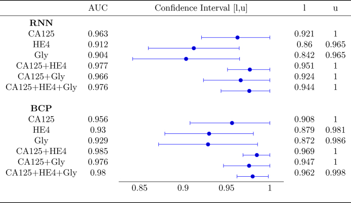
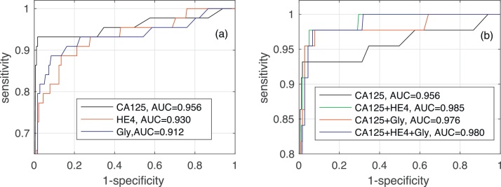
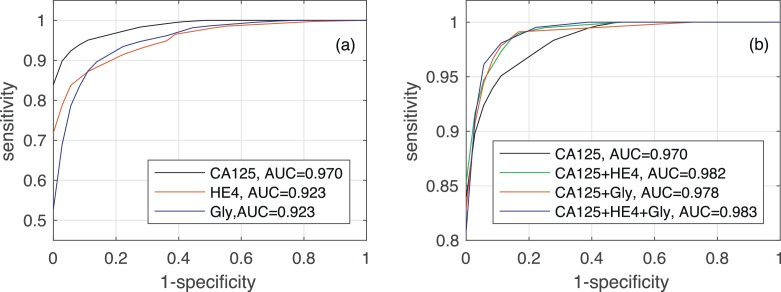
Fig. 4 shows the AUC along with the corresponding confidence interval for every individual biomarker, as well as every combination of biomarkers encompassing CA125. In both algorithms it is clear that, when considering a single biomarker, CA125 is the one yielding the best performance (a larger AUC in a narrower confidence interval). When using several biomarkers, the best results are obtained when combining CA125 with HE4. Specifically, in both algorithms the AUCs for “CA125+HE4” and “CA125+HE4+Gly” are ≈0.98. Fig. 5, Fig. 6 show, respectively, the ROC curves for the BCP and RNN schemes. In both cases, the plot on the left focuses on the results for a single biomarker, while the plot on the right depicts the curves for combinations of biomarkers (along with the curve of CA125 that serves as a reference).

Fig. 4.

Area Under the Curve with 95% confidence intervals.

Fig. 5.

ROC curves and area under ROC curve obtained by the Bayesian Change-point method for different biomarkers: (a) when considering a single biomarker (CA125, HE4 or glycodelin), (b) when considering different combinations of then three biomarkers.

Fig. 6.

ROC curves and area under ROC curve obtained by the Recurrent Neural Network for different biomarkers: (a) when considering a single biomarker (CA125, HE4 or glycodelin), (b) when considering different combinations of the three biomarkers.

The confidence intervals given in Fig. 4 suggest that the differences between the AUC within and across algorithms are not statistically significant. Specifically, when comparing both schemes (the one based on RNNs and the one based on BCP) for a standalone biomarker or combination of biomarkers, the estimated AUCs are very close and the corresponding confidence intervals overlap to a great extent. Hence, it is hard to say one algorithm performs better than the other. On the other hand, when focusing on a certain algorithm, although using the three biomarkers increases the AUC and narrows down the 95% confidence interval, there is still some overlap when the latter is compared with the confidence intervals for individual biomarkers.

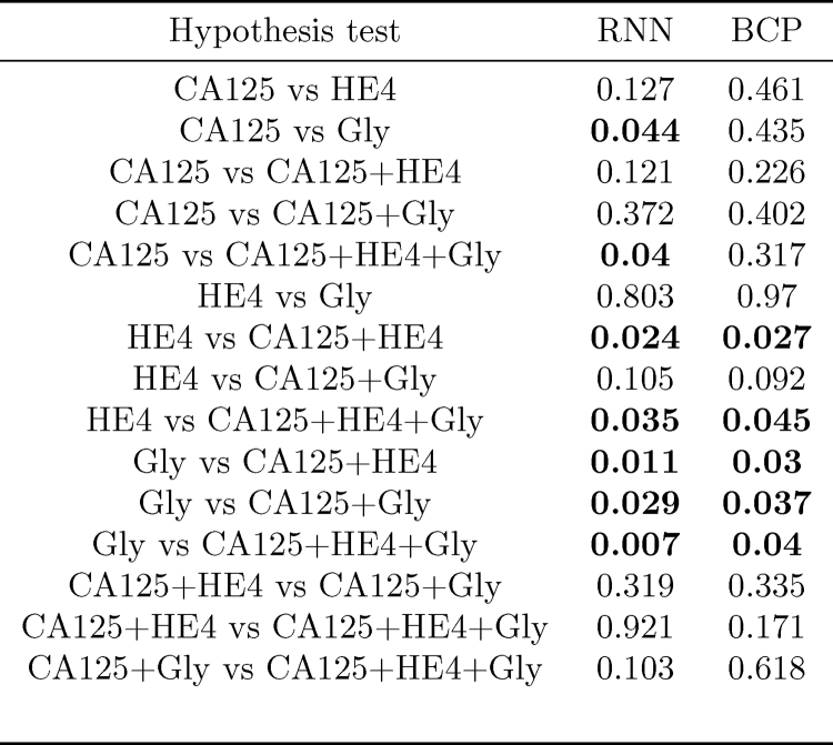
In order to assess whether, for a given algorithm, the differences between AUCs for different combinations of biomarkers are statistically significant, we have computed the p-value of hypothesis tests comparing, pairwise, every possible combination of biomarkers. Notice that here we are slightly abusing notation, and we are also referring to a single biomarker, e.g., “CA125”, as a combination. The results are shown in Fig. 7. Those tests in which the null hypothesis (“the compared AUCs are equal”) is rejected at a 0.05 significance level are highlighted in bold font. Some remarks are in order

• •In both algorithms, the AUC attained using the three biomarkers is different (better) from that achieved using only HE4 or only Gly; additionally, in the RNN-based algorithm, it is also the case that using all the biomarkers yields an improved AUC as compared to using only CA125.
• •In both algorithms the AUC using only Gly is different from that using any of the two-marker combinations; in the RNN algorithm the hypothesis that the AUC using only Gly is the same as that using only CA125 is also rejected.
• •In both algorithms, we must also reject the hypothesis that the results for HE4 only are equal to those obtained using “CA125+HE4” combination.

Fig. 7.

p-Values obtained for the hypothesis tests assessing whether the AUCs attained by different combinations of biomarkers are different (in both the RNN- and BCP-based methods).

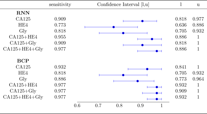
For the problem at hand, one of the most important performance metrics is the sensitivity. In order to compare effectiveness of BCP- and RNN-based schemes for this metric, we set the corresponding decision threshold of each algorithm at a value such that a minimum specificity of 90% is attained, and evaluate the sensitivity afterwards. The results are shown in Figure 8.

Fig. 8.

Sensitivity for a 90% specificity.

When a single biomarker is used, the sensitivity of the BCP algorithm is slightly higher than that exhibited by the RNN in each of the three cases (CA125, HE4, and Gly), although the corresponding confidence intervals overlap pairwise, and hence the differences are not statistically significant. When using combination of biomarkers, both algorithms show a noticeable increase in the sensitivity. Specifically, when considering the three biomarkers, both the RNN and the BCP algorithm exhibit a sensitivity of around 0.98, whereas when only CA125 is exploited, the sensitivity attained by the RNN algorithm is ≈0.91 and that achieved by the BCP-based scheme is ≈0.93. In both algorithms, there is overlap between the confidence intervals for CA125 and CA125+HE4+Gly, but it is clear that using the combination the confidence interval is significantly narrower. Hence, it could be argued that both algorithms benefit from using all the three biomarkers.

6. Discussion and conclusions

We have explored two different approaches to tackle the problem of ovarian cancer detection from a sequence of longitudinal measurements of several biomarkers. The first approach relies on a Bayesian hierarchical model whose fundamental assumption is that measurements taken from case subjects exhibit a changepoint in one or several biomarkers. The second approach is a purely discriminative machine learning algorithm based on the use of RNNs, a kind of artificial neural network specially suited for the processing of ordered sequences of data.

Our experimental results (relying on real data) show that, regardless of the method, CA125 is the single biomarker yielding the best performance, as measured by either the AUC or the sensitivity attained for a fixed specificity. When using several biomarkers, both algorithms get a performance boost, although the latter is not always statistically significant. For instance, 95% confidence level hypothesis tests suggest that the joint use of CA125, HE4 and glycodelin biomarkers increases the performance of both methods as compared to using either HE4 or glycodelin alone. However, only for the RNN-based scheme, the combination of the three biomarkers seems to improve the AUC obtained by CA125 alone. In any case, both methods exhibit nearly the same performance. Similar conclusions can be drawn when looking at the sensitivity of the algorithms for a fixed specificity at 90%. In such a case, the confidence interval for the sensitivity obtained using CA125 alone, on one hand, and the three biomarkers, on the other hand, overlap. Hence we cannot rule out the hypothesis that both sensitivities are equal. However, when using CA125, HE4 and glycodelin, the estimated sensitivity is noticeably higher and, moreover, the corresponding confidence interval is markedly narrower.

Since the performances of the two approaches are ultimately comparable when every available biomarker is used, other considerations must be taken into account when choosing one over the other. If interpretability is a concern, the parameters estimated by the BCP algorithm have a physical intuitive interpretation, whereas the weights in a neural network (NN) are usually much harder to interpret. On the other hand, RNNs are able to integrate different markers more naturally. In connection with this, RNNs might also be able to perform some kind of feature selection by way of weighting more heavily a certain biomarker (accounting for previously seen values) whereas in the BCP scheme, every biomarker is considered equally important.

RNNs, and NNs in general, usually need a large amount of training data in order to obtain a model that achieves good generalization capabilities. In order to avoid overfitting, regularization techniques, such as dropout, can be used when the dataset is small, but it is not always straightforward how or where to apply them. On the contrary, generative models like BCP make the most of the available data while accounting for the uncertainty given by the prior.

Regarding the RNN approach, future works should use a larger dataset which will allow to exploit the full potential of deep learning in the problem at hand. Also, many other NN architectures are possible, but exploring them would demand a paper of its own.

References

- 1.http://cancerresearchuk
- 2.Skates S.J., Menon U., MacDonald N., Rosenthal A.N., Oram D.H., Knapp R.C., Jacobs I.J. Calculation of the risk of ovarian cancer from serial CA-125 values for preclinical detection in postmenopausal women. J. Clin. Oncol. 2003;21:206–211. doi: 10.1200/JCO.2003.02.955. [DOI] [PubMed] [Google Scholar]
- 3.Jacobs I., Menon U. Progress and challenges in screening for early detection of ovarian cancer. Molec. Cell. Proteomics. 2004;3:355–366. doi: 10.1074/mcp.R400006-MCP200. [DOI] [PubMed] [Google Scholar]
- 4.Bosse K., Rhiem K., Kerstin B., Wappenschmidt M., Hellmich M., Madeja M., Ortmann P., Mallmann R., Schmutzler Screening for ovarian cancer by transvaginal ultrasound and serum CA125 measurement in women with a familial predisposition: a prospective cohort study. Gynecol. Oncol. 2006;103:1077–1082. doi: 10.1016/j.ygyno.2006.06.032. [DOI] [PubMed] [Google Scholar]
- 5.Blyuss O., Burnell M., Ryan A., Gentry-Maharaj A., Mariño I.P., Kalsi J., Manchanda R., Timms J.F., Parmar M., Skates S.J., Jacobs I., Zaikin A., Menon U. Comparison of longitudinal CA125 algorithms as a first line screen for ovarian cancer in the general population. Clin. Cancer Res. 2018 doi: 10.1158/1078-0432.CCR-18-0208. [DOI] [PMC free article] [PubMed] [Google Scholar]
- 6.Mariño I.P., Blyuss O., Ryan A., Gentry-Maharaj A., Timms J.F., Dawnay A., Kalsi J., Jacobs I., Menon U., Zaikin A. Change-point of multiple biomarkers in women with ovarian cancer. Biomed. Signal Proc. and Control. 2017;33:169–177. [Google Scholar]
- 7.Moore R.G., McMeekin D.S., Brown A.K., DiSilvestro P., Miller M.C. A novel multiple marker bioassay utilizing HE4 and CA125 for the prediction of ovarian cancer in patients with a pelvic mass. Gynecol. Oncol. 2009;112:40–46. doi: 10.1016/j.ygyno.2008.08.031. [DOI] [PMC free article] [PubMed] [Google Scholar]
- 8.Karlsen M.A., Høgdall E.V., Christensen I.J., Borgfeldt C., Kalapotharakos G., Zdrazilova-Dubska L., Chovanec J., Lok C.A., Stiekema A., Mutz-Dehbalaie I., Rosenthal A.N., Moore E.K., Schodin B.A., Sumpaico W.W., Sundfeldt K., Kristjansdottir B., Zapardiel I., Høgdall C.K. A novel diagnostic index combining HE4, CA125 and age may improve triage of women with suspected ovarian cancer – an international multicenter study in women with an ovarian mass. Gynecol. Oncol. 2015;138:640–646. doi: 10.1016/j.ygyno.2015.06.021. [DOI] [PubMed] [Google Scholar]
- 9.Van Gorp T., Cadron I., Despierre E. HE4 and CA125 as a diagnostic test in ovarian cancer: prospective validation of the Risk of Ovarian Malignancy Algorithm. Br. J. Cancer. 2011;104:863–870. doi: 10.1038/sj.bjc.6606092. [DOI] [PMC free article] [PubMed] [Google Scholar]
- 10.Ghasemi N., Ghobadzadeh S., Zahraei M. HE4 combined with CA125: favorable screening tool for ovarian cancer. Med. Oncol. 2014;31 doi: 10.1007/s12032-013-0808-0. article 808. [DOI] [PubMed] [Google Scholar]
- 11.Anderson G.L., McIntosh M., Wu L. Assessing lead time of selected ovarian cancer biomarkers: a nested case–control study. J. Natl. Cancer Inst. 2010;102:26–38. doi: 10.1093/jnci/djp438. [DOI] [PMC free article] [PubMed] [Google Scholar]
- 12.Blyuss O., Gentry-Maharaj A., Fourkala E.-O., Ryan A., Zaikin A., Menon U., Jacobs I., Timms J.F. Serial patterns of ovarian cancer biomarkers in a prediagnosis longitudinal dataset. BioMed. Res. Int. 2015;2015:681416. doi: 10.1155/2015/681416. [DOI] [PMC free article] [PubMed] [Google Scholar]
- 13.Zhao T., Hu W. CA125 and HE4: measurement tools for ovarian cancer. Gynecol. Obst. Invest. 2016;81:430–435. doi: 10.1159/000442288. [DOI] [PubMed] [Google Scholar]
- 14.Guo J., Yu J., Song X., Mi H. Serum CA125, CA199 and CEA combined detection for epithelial ovarian cancer diagnosis: a meta-analysis. Open Med. 2017;12:131–137. doi: 10.1515/med-2017-0020. [DOI] [PMC free article] [PubMed] [Google Scholar]
- 15.Montagnana M., Danese E., Ruzzenente O. The ROMA (Risk of Ovarian Malignancy Algorithm) for estimating the risk of epithelial ovarian cancer in women presenting with pelvic mass: is it really useful? Clin. Chem. Lab. Med. 2011;49:521–525. doi: 10.1515/CCLM.2011.075. [DOI] [PubMed] [Google Scholar]
- 16.Buys S.S., Partridge E., Black A. Effect of screening on ovarian cancer mortality: the Prostate, Lung, Colorectal and Ovarian (PLCO) cancer screening randomized controlled trial. J. Am. Med. Assoc. 2011;305:2295–2302. doi: 10.1001/jama.2011.766. [DOI] [PubMed] [Google Scholar]
- 17.Moore R.G., Brown A.K., Miller M.C., Skates S., Allard W.J., Verch T., Steinhoff M., Messerlian G., DiSilvestro P., Granai C.O., Bast R.C., Jr. The use of multiple novel tumor biomarkers for the detection of ovarian carcinoma in patients with a pelvic mass. Gynecol. Oncol. 2008;108:402–408. doi: 10.1016/j.ygyno.2007.10.017. [DOI] [PubMed] [Google Scholar]
- 18.Cramer D.W., Bast R.C., Jr., Berg C.D., Diamandis E.P., Godwin A.K., Hartge P., Lokshin A.E., Lu K.H., McIntosh M.W., Mor G., Patriotis C., Pinsky P.F., Thornquist M.D., Scholler N., Skates S.J., Sluss P.M., Srivastava S., Ward D.C., Zhang Z., Zhu C.S., Urban N. Ovarian cancer biomarker performance in prostate, lung, colorectal, and ovarian cancer screening trial specimens. Cancer Prevent. Res. 2011;4(3):365–374. doi: 10.1158/1940-6207.CAPR-10-0195. [DOI] [PMC free article] [PubMed] [Google Scholar]
- 19.Bischof A., Briese V., Richter D.-U., Bergemann C., Friese K., Jeschke U. Measurement of glycodelin A in fluids of benign ovarian cysts, borderline tumours and malignant ovarian cancer. Anticancer Res. 2005;25:1639–1644. [PubMed] [Google Scholar]
- 20.Havrilesky L.J., Whitehead C.M., Rubatt J.M. Evaluation of biomarker panels for early stage ovarian cancer detection and monitoring for disease recurrence. Gynecol. Oncol. 2008;110:374–382. doi: 10.1016/j.ygyno.2008.04.041. [DOI] [PubMed] [Google Scholar]
- 21.Skates S.J., Pauler D.K., Jacobs I.J. Screening based on the risk of cancer calculation from Bayesian hierarchical change-point and mixture models of longitudinal markers. J. Am. Stat. Assoc. 2001;96:429–439. [Google Scholar]
- 22.UKCTOCS . 2003. International Standard Randomised Controlled Trial, number ISRCTN22488978; NCT00058032.https://clinicaltrials.gov/ [Google Scholar]
- 23.Goodfellow I., Bengio Y., Courville A. MIT Press; 2016. Deep Learning. [Google Scholar]
- 24.Graves A., Liwicki M., Bunke H., Schmidhuber J., Fernández S. Unconstrained on-line handwriting recognition with recurrent neural networks. Adv. Neural Inf. Process. Syst. 2008:577–584. [Google Scholar]
- 25.Graves A., Mohamed A.-R., Hinton G. Speech recognition with deep recurrent neural networks, IEEE International Conference on Acoustics. Speech Signal Process. 2013:6645–6649. [Google Scholar]
- 26.Vinyals O., Toshev A., Bengio S., Erhan D. Show and tell: a neural image caption generator. Proceedings of the IEEE conference on Computer Vision and Pattern Recognition. 2015:3156–3164. [Google Scholar]
- 27.Lipton Z.C., Kale D.C., Elkan C., Wetzell R. 2015. Learning to Diagnose with LSTM Recurrent Neural Networks. arXiv preprint arXiv:1511.03677. [Google Scholar]
- 28.Aczon M., Ledbetter D., Ho L., Gunny A., Flynn A., Williams J., Wetzel R. 2017. Dynamic Mortality Risk Predictions in Pediatric Critical Care Using Recurrent Neural Networks. arXiv preprint arXiv:1701.06675. [Google Scholar]
- 29.Choi E., Schuetz A., Stewart W.F., Sun J. Using recurrent neural network models for early detection of heart failure onset. J. Am. Med. Inf. Assoc. 2016;24:361–370. doi: 10.1093/jamia/ocw112. [DOI] [PMC free article] [PubMed] [Google Scholar]
- 30.Singh R.R., Conjeti S., Banerjee R. A comparative evaluation of neural network classifiers for stress level analysis of automotive drivers using physiological signals. Biomed. Signal Proc. Control. 2013;8:740–754. [Google Scholar]
- 31.FIGO (International Federation of Gynecology and Obstetrics). http://www.figo.org.
- 32.Rastogi M., Gupta S., Sachan M. Biomarkers towards ovarian cancer diagnostics: present and future prospects. Braz. Arch. Biol. Technol. 2016;59 [Google Scholar]
- 33.Ueland F.R. A perspective on ovarian cancer biomarkers: past, present and yet-to-come. Diagnostics. 2017;7:14. doi: 10.3390/diagnostics7010014. [DOI] [PMC free article] [PubMed] [Google Scholar]
- 34.Roberts G.O., Rosenthal J.S. Harris recurrence of Metropolis-within-Gibbs and trans-dimensional Markov chains. Ann. Appl. Prob. 2006;16:2123–2139. [Google Scholar]
- 36.Saxe A.M., McClelland J.L., Ganguli S. 2013. Exact Solutions to the Nonlinear Dynamics of Learning in Deep Linear Neural Networks. arXiv preprint arXiv:1312.6120. [Google Scholar]
- 37.Glorot X., Bengio Y. Understanding the difficulty of training deep feedforward neural networks. Proceedings of the Thirteenth International Conference on Artificial Intelligence and Statistics. 2010:249–256. [Google Scholar]