Development and Validation of a Deep Neural Network Model for Prediction of Postoperative In-Hospital Mortality

Abstract

Background

We tested the hypothesis that deep neural networks trained on intraoperative features can predict postoperative in-hospital mortality.

Methods

The data used to train and validate the algorithm consists of 59,985 patients with 87 features extracted at the end of surgery. Feed-forward networks with a logistic output were trained using stochastic gradient descent with momentum. The deep neural networks were trained on 80% of the data, with 20% reserved for testing. We assessed improvement of the deep neural network by adding American Society of Anesthesiologists Physical Status Classification and robustness of the deep neural network to a reduced feature set. The networks were then compared to Physical Status, logistic regression, and other published clinical scores including the Surgical Apgar, PreOperative Score to Predict PostOperative Mortality, Risk Quantification Index, and the Risk Stratification Index.

Results

In-hospital mortality in the training and test sets were 0.81% and 0.73%. The deep neural network with a reduced feature set and Physical Status classification had the highest area under the receiver operating characteristics curve, 0.91 (95% CI, 0.88 – 0.93). The highest logistic regression area under the curve was found with a reduced feature set and ASA status (0.90, 95% CI. 0.87 – 0.93). The Risk Stratification Index had the highest area under the receiver operating characteristics curve, at 0.97 (95% CI, 0.94 – 0.99).

Conclusion

Deep neural networks can predict in-hospital mortality based on automatically extractable intraoperative data, but are not (yet) superior to existing methods.

Introduction

About 230 million surgeries are performed annually worldwide.¹ While the postoperative mortality is low, less than 2%, about 12% of all patients -the high-risk surgery group- account for 80% of postoperative deaths.^2,3 To assist in guiding clinical decisions and prioritization of care, several perioperative clinical and administrative risk scores have been proposed.

The goal of perioperative clinical risk scores is to help guide care in individual patients by planning clinical management and allocating resources. The goal of perioperative administrative risk scores (based on diagnoses and procedures) is to help compare hospitals. In the perioperative setting, frequently used risk scores include the American Society of Anesthesiologists Physical Status Classification (ASA, a preoperative score) and the Surgical Apgar score.^4,5 The ASA score was developed in 1963 and remains widely used.⁴ Its main limitation is that it is subjective, it presents with high inter- and intra-rater variability, it cannot be automated, and it relies on clinicians’ experience. The Surgical Apgar score (an intraoperative score) uses three variables: estimated blood loss, lowest mean arterial pressure, and lowest heart rate during surgery to predict major postoperative complications.⁵ Favored for its simplicity, the Surgical Apgar score presents with area under the receiver operating characteristics curve (AUC) ranging from 0.6 to 0.8 for major complications or death with a correlation varying with subspecialty.^6–9 In addition, the Surgical Apgar score has been shown to not substantially improve mortality risk stratification when combined with preoperative scores.⁹ In response to these limitations, there has been work to create more objective and accurate scores. The most popular method used to develop new scoring systems is based on logistic regression, such as the PreOperative Score to Predict Postoperative Mortality (POSPOM).¹⁰ In order to make these scores accessible in clinical practice, the logistic regression coefficients are normalized to easily summed values to be interpreted as a score rather than the direct logistic regression output. Besides the above mentioned clinical risk scores, other recent perioperative administrative risk scores are the Risk Stratification Index (RSI) (published initially in 2010¹¹ and validated in 2017 on nearly 40 Million patients¹²) and the Risk Quantification Index (RQI)¹³.

In recent years, and although they are not new¹¹, neural networks and deep neural networks, known as “deep learning”, have been used to tackle a variety of problems, ranging from computer vision^12–17, gaming^18–20, high-energy physics^21,22, chemistry^23–25, and biology^26–28. While there have been studies using other machine learning methods for clinical applications such as predicting cardiorespiratory instability^29,30 and 30-day readmission^31,32, the use of deep neural networks (DNN) in medicine is relatively limited.^33–36

In this manuscript, we present the development and validation of a deep neural network (DNN) model based upon intraoperative clinical features, to predict postoperative in-hospital mortality in patients undergoing surgery under general anesthesia. Its performance is presented together with other published clinical risk scores and administrative risk scores, as well as a logistic regression model using the same intraoperative features as the DNN. The DNNs were also assessed for leveraging preoperative information by the addition of ASA and POSPOM as features.

Materials and Methods

This manuscript follows the “Guidelines for Developing and Reporting Machine Learning Predictive Models in Biomedical Research: A Multidisciplinary View”³⁷.

Electronic Medical Record (EMR) Data Extraction

All data for this study were extracted from the Perioperative Data Warehouse (PDW), a custom built robust data warehouse containing all patients who have undergone surgery at UCLA since the implementation of the electronic medical record (EMR) (EPIC Systems, Madison WI) on March 17^th, 2013. The construction of the PDW has been previously described³⁸. Briefly the PDW has a two-stage design. In the first stage data are extracted from EPIC’s Clarity database into 26 tables organized around three distinct concepts: patients, surgical procedures and health system encounters. These data are then used to populate a series of 800 distinct measures and metrics such as procedure duration, readmissions, admission International Statistical Classification of Diseases (ICD) codes, and others. All data used for this study were obtained from this data warehouse and IRB approval (IRB#15-000518) has been obtained for this retrospective review.

A list of all surgical cases performed between March 17, 2013 and July 16, 2016 were extracted from the PDW. The UCLA Health System includes two inpatient medical centers as well as three ambulatory surgical centers, however only cases performed in one of the two-inpatient hospitals (including operating room and “off-site” locations) under general anesthesia were included in this analysis. Cases on patients younger than 18 years of age or older than 89 years of age were excluded. In the event that more than one procedure was performed during a given health system encounter only the first case was included.

Model Endpoint Definition

The occurrence of an in-hospital mortality was extracted as a binary event [0, 1] based upon either the presence of a “mortality date” in the EMR between surgery time and discharge or a discharge disposition of expired combined with a note associated with the death (i.e. death summary, death note). The definition of in-hospital mortality was independent of length of stay in the hospital.

Model Input Features

Each surgical record corresponded to a unique hospital admission and contained 87 features calculated or extracted at the end of surgery (Table 1). These features were considered to be potentially predictive of in-hospital mortality by clinicians’ consensus (I.H., M.C., E.G.) and included descriptive intraoperative vital signs, such as minimum and maximum blood pressure values; summary of drugs and fluids interventions such as total blood infused and total vasopressin administered; as well as patient anesthesia descriptions such as presence of an arterial line and type of anesthesia (all features are detailed in Table 1).

Table 1.

Eighty seven features used in models with description and applied maximum possible values as defined by domain experts. The 45 features used in the reduced feature set are indicated with an*.

Feature Name(s)	Description	# Features; # Features in Reduced Feature Set	Maximum Possible Absolute Value (if applicable)
COLLOID_ML*	Total Colloid Transfused (ml)	1; 1	-
CRYSTALLOID_ML*	Total Crystalloid Transfused (ml)	1; 1	-
DBP MAX*, MIN*, AVG, MED, STD	Maximum, Minimum, Average, Median, and Standard Deviation Diastolic Blood Pressure for the case (mmHg)	5; 2	150
DBP_10min MAX, MIN, AVG, MED, STD	Maximum, Minimum, Average, Median, and Standard Deviation Diastolic Blood Pressure for the last 10 minutes of the case (mmHg)	5; 0	150
EBL*	Total Estimated Blood Loss (ml)	1; 1	-
EPHEDRINE BOLUS*	Total bolus dose of Ephedrine (mg) during the case	1; 1	-
EPINEPHRINE BOLUS*, END RATE*, MAX RATE*	Total bolus dose (mcg), End of case infusion rate (mcg/kg/min), and Highest infusion rate (mcg/kg/min) of Epinephrine during the case	3; 3	-
ESMOLOL BOLUS*, END RATE*, MAX RATE*	Total bolus dose (mg), End of case infusion rate (mcg/kg/min), and Highest Infusion rate (mcg/kg/min) of Esmolol during the case	3; 3	-
HR MAX*, MIN*, AVG, MED, STD	Maximum, Minimum, Average, Median, and Standard Deviation Heart Rate (bpm) for the case	5; 2	180
HR_10min MAX, MIN, AVG, MED, STD	Maximum, Minimum, Average, Median, and Standard Deviation Heart Rate (bpm) for the last 10 minutes of the case	5; 0	180
INVASIVE_LINE_YN*	Invasive Central venous, arterial, or Pulmonary Arterial Line used for the case (Yes/No)	1; 1	-
MAP MAX*, MIN*, AVG, MED, STD	Maximum, Minimum, Average, Median, and Standard Deviation Mean Blood Pressure (mmHg) for the case	5; 2	300
MAP_10min MAX, MIN, AVG, MED, STD	Maximum, Minimum, Average, Median, and Standard Deviation Mean Blood Pressure (mmHg) for the last 10 minutes of the case	5; 0	300
DES MAX*	Maximum Minimum alveolar concentration of desflurane during the case (note this is not age adjusted)	1; 1	12
GLUCOSE MAX*, MIN*	Maximum and Minimum plasma Glucose concentration for the Case (mg/dl)	2; 2	400
ISO MAX*	Maximum Minimum alveolar concentration of isoflurane during the case (note this is not age adjusted)	1; 1	12
SEVO MAX*	Maximum Minimum alveolar concentration of sevoflurane during the case (note this is not age adjusted)	1; 1	10
MILRINONE END RATE*, MAX RATE*	End of case Infusion Rate and Highest Infusion rate of Milrinone during the case (mcg/kg/min)	2; 2	-
HGB MIN*	Minimum Hemoglobin concentration (g/dl) during the case	1; 1	15
MINUTES MAP < 50	Cumulative minutes with mean arterial pressure <50 mmHg (min)	1; 0	-
MINUTES MAP < 60	Cumulative minutes with mean arterial pressure < 60 mmHg (min)	1; 0	-
NICARDIPINE END RATE*, MAX RATE*	End of case infusion Rate and Highest Infusion Rate of Nicardipine during the case (mg/hr)	2; 2	-
NITRIC_OXIDE_YN*	Nitric Oxide Used for the Case (Yes/No)	1; 1	-
NITROGLYCERIN BOLUS*, END RATE*, MAX RATE*	Total bolus dose (mcg), End of case infusion rate (mcg/min), and Highest Infusion rate (mcg/min) of Nitroglycerin during the case	3; 3	-
NITROPRUSSIDE END RATE*, MAX RATE*	End of case infusion Rate and Highest Infusion Rate of Nitroprusside (mcg/kg/min) during the case	2; 2	-
PHENYLEPHRINE BOLUS*, END RATE*, MAX RATE*	Total bolus dose (mcg), End of case infusion rate (mcg/min), and Highest Infusion rate (mcg/min) of Phenylephrine during the case	3; 3	-
SBP MAX*, MIN*, AVG, MED, STD	Maximum, Minimum, Average, Median, and Standard Deviation Systolic blood pressure (mmHg) for the case	5; 2	300
SBP_10min MAX, MIN, AVG, MED, STD	Maximum, Minimum, Average, Median, and Standard Deviation Systolic blood pressure (mmHg) for the last 10 minutes of the case	5; 0	300
SpO2 MAX*, MIN*, AVG, MED, STD	Maximum, Minimum, Average, Median, and Standard Deviation SpO2 (%) for the case	5; 2	100
SpO2_10min MAX, MIN, AVG, MED, STD	Maximum, Minimum, Average, Median, and Standard Deviation SpO2 (%) for the last 10 minutes of the case	5; 0	100
UOP*	Total Urine Output (ml)	1; 1	-
VASOPRESSIN BOLUS*, END RATE*, MAX RATE*	Total bolus dose (units), End of case infusion rate (units/hr), and Highest Infusion rate (units/hr) of Vasopressin during the case	3; 3	-
XFUSION_RBC_ML*	Total Red Blood Cells Transfused (ml)	1; 1	-
	Total # Features	87; 45

Data Preprocessing

Prior to model development, missing values were filled with the mean value for the respective feature. In addition, to account for observations where the value is clinically out of range, values greater than a clinically normal maximum were set to a maximum possible value (Table 1). These out of range values were due to the data artifact in the raw EMR data. For example, a systolic blood pressure of 400 mmHg is not clinically possible, however, it may be recognized as the maximum systolic blood pressure for the case during EMR extraction. The data was then randomly divided into training (80%) and test (20%) data sets, with equal % occurrence of in-hospital mortality. Training data was rescaled to have a mean of 0 and standard deviation of 1 per feature. Test data was rescaled with the training data mean and standard deviation.

Development of the Model

In this work, we were interested in classifying patients at risk of in-hospital mortality using deep neural networks (DNNs), also referred to as deep learning. During development of DNNs, there are many unknown model parameters that need to be optimized by the DNN during training. These model parameters are first initialized and then optimized to decrease the error of the model’s output to correctly classify in-hospital mortality. This error is referred to as a loss function. The type of DNN used in this study is a feedforward network with fully connected layers and a logistic output. “Fully connected” refers to the fact that all neurons between two adjacent layers are fully pairwise connected. A logistic output was chosen so that the output of the model could be interpreted as probability of in-hospital mortality [0-1]. To develop a DNN, it is important to fine-tune the hyperparameters as well as the architecture. We utilized stochastic gradient descent (SGD) with momentums [0.8, 0.85, 0.9, 0.95, 0.99] and initial learning rates [0.01, 0.1, 0.5], and a batch size of 200. We also assessed DNN architectures of 1 to 5 hidden layers with 10 – 300 neurons per layer, and rectified linear unit (ReLU) and hyperbolic tangent (tanh) activation functions. The loss function was cross entropy. We utilized five-fold cross validation with the training set (80%) to select the best hyperparameters and architecture based on mean cross validation performance. These best hyperparameters and architecture were then used to train a model on the entire training set (80%) prior to testing final model performance on the separate test set (20%).

i Overfitting

In addition, overfitting was a major concern in the development of our model. While ~50,000 patients is large for clinical data, it is small relative to datasets typically found in deep learning tasks such as vision and speech recognition where millions of samples are available. Thus, regularization was critical. To address this, we utilized three methods: 1) early stopping, 2) L2 weight decay, and 3) dropout. Early stopping is the halting of model training when the loss of a separate early stopping validation set starts to increase compared to the training loss, indicating overfitting. This early stopping validation set was taken as a random 20% of the training set, and a patience of 10 epochs was utilized. L2 weight decay is a method of limiting the size of the weight of every parameter. The standard L2 weight penalty involves adding an extra term to the loss function that penalizes the squared weights, keeping the weights small unless the error derivative is big. We utilized an L2 weight penalty of 0.0001. Dropout is a method where neurons are removed from the network with a specified probability, to prevent co-adapting of the neurons.^39–41 Dropout was applied to all layers with a probability of 0.5.

ii Data Augmentation

The goal of training was to optimize model parameters to decrease classification error of in-hospital mortality. However, the actual percent of occurrence of in-hospital mortality in the data was low and thus the data was skewed. The % occurrence of mortality in the training dataset was < 1%. To help with this skewed distribution, training data was augmented by taking only the observations positive for in-hospital mortality and adding Gaussian noise. This was performed by adding a random number taken from a Gaussian distribution with a standard deviation of 0.0001 to each feature’s value. This essentially duplicated the in-hospital mortality observations with a slight perturbation. The in-hospital mortality observations in the training data set were augmented using this method to approximately 45% occurrence prior to training. During cross validation, this meant that only training folds were augmented. The validation fold was not augmented.

Feature Reduction and Preoperative Feature Experiments

Experiments to assess the impact of 1) reducing the number of features from the clinician chosen 87 to 45 features, and 2) adding ASA and POSPOM as a feature were also conducted. The reduced 45 feature set was created by excluding all “derived” features, specifically average, median, standard deviation, and last 10 minutes of the surgical case features (Table 1).

After choosing the best performing DNN architecture and hyperparameters with the complete 87 features data set, five additional DNNs were each trained with the following:

1. the addition of ASA as a model feature (88 features)

2. the addition of POSPOM as a model feature (88 features)

3. a reduced model feature set (45 features)

4. the addition of ASA to the reduced feature set (46 features).

5. the addition of POSPOM to the reduced feature set (46 features).

Model Performance

All model performances were assessed on 20% of the data held out from training as a test set. Model performance was compared to ASA, Surgical Apgar, RQI, RSI, POSPOM, and a standard logistic regression model using the same combination of features as in the DNN. ASA was extracted from the UCLA preoperative assessment record. Surgical Apgar was calculated using Gawande et al.⁵ RQI could not be calculated using the downloadable R package from Cleveland Clinic’s website <http://my.clevelandclinic.org/departments/anesthesiology/depts/outcomes-research> due to technical issues with the R version, and so RQI log probability and score were calculated from equations provided in Sigakis et al.⁴² Uncalibrated RSI was calculated using coefficients provided by the original authors (Appendix 1).⁴³ To calculate RSI, all International Statistical Classification of Diseases, 9^th revision (ICD-9) diagnosis codes for each patient were matched with an RSI coefficient and the coefficients were then summed. POSPOM scores were extracted from the PDW, where they were calculated as described by Le Manach et al.¹⁰ Each of the diseases described by Le Manach et al.¹⁰ were extracted as a binary endpoint from the admission ICD codes for the relevant hospital admission. In addition to assigning points based on patient co-morbidities the POSPOM also assigns points for the type of surgery performed. These points were assigned based on the primary surgical service for the given procedure.

i Area Under the Receiver Operating Characteristics (ROC) Curves

Model performance was assessed using Area Under the ROC Curve (AUC) and 95% confidence intervals for AUC were calculated using bootstrapping with 1,000 samples.

ii Choosing a Threshold

The F1 score, sensitivity, and specificity were calculated for different thresholds for the DNN models, logistic regression model, ASA, and POSPOM. The F1 score is a measure of precision and recall, ranging from 0 to 1. It is calculated as $F1=2\ast \frac{\mathit{precision}\ast \mathit{recall}}{\mathit{precision}+\mathit{recall}}$ , where precision is (true positives/predicted true) and recall is equivalent to sensitivity. Two different threshold methods were assessed: 1) a threshold that optimized the observed in-hospital mortality rate and 2) a threshold based on the highest F1 score. The number of true positives, true negatives, false positives, and false negatives were then assessed for each threshold to assess differences in the number of patients correctly predicted by each model.

iii Calibration

Calibration was performed to account for the use of data augmentation on the training data set to be used during training of the DNN. This data augmentation served to balance classes in the training data set to approximately 45% mortality vs the true distribution of mortality (<1%). This extreme augmentation of the training data set classes skewed predicted probabilities to be higher than the expected probability based on the true distribution of mortality (<1%). Therefore, we performed calibration after finalizing the model. Calibration was performed only on the test data set. Calibration of the DNN predicted probability output was performed using the following equation:

$$\mathit{Calibrated}\mathit{Predicted}\mathit{Probability}=\frac{1}{1+\left(\frac{1}{\mathit{Predicted}\mathit{Probability}}-1\right)\frac{P\left(0\right)}{P\left(1\right)}}$$

, where $P\left(1\right)= \frac{\# \mathit{Observed} \mathit{Mortality} in \mathit{Test} }{\# \mathit{Test} \mathit{Patients}}=\frac{87}{11997}$ and $P\left(0\right)= 1-P\left(1\right)$. This calibration formula was used to maintain the rank of predicted probabilities, and thus not changing any model performance metrics (AUC, sensitivity, specificity, or F1 score).

In addition, calibration plots and Brier scores were used to assess calibration of predictions.

iv Feature Importance

To assess which features are the most predictive in the DNN, we performed a feature ablation analysis. This analysis consisted of removing model features grouped by type of clinical feature, and then re-training a DNN with the same final architecture as well as hyperparameters on the remaining features. The change in AUC with the removal of each feature was then assessed to evaluate the importance of each group of features. To assess which features are the most predictive in the logistic regression model, we assessed which features corresponded to the largest weights.

All DNN models were developed and applied using Keras.⁴⁴ Logistic regression models and performance metrics were calculated with scikit-learn.⁴⁵

Results

Patient characteristics

The data consisted of 59,985 surgical records total. Patient demographics and characteristics of the training and test data sets are summarized in Table 2. The in-hospital mortality rate of both the training and test set is less than 1%. The presence of invasive lines is also similar for both sets (26.5% in training; 26.7% in test). The most prevalent ASA is 3 at 49.9% for both sets.

Table 2.

Training and test data set patient characteristics reported as number patients (%) or mean ± standard deviation. HCUP code description and distribution is shown only for those representing >1% of the train data set.

	Train	Test
# of Patients	47,988	11,997
# of Patients with In Hospital Mortality (%)	389 (0.81%)	87 (0.73%)
Age (years)	56 ± 17	56 ± 18
Estimated Blood loss (cc)	95 ± 540	94 ± 410
Presence of Arterial Line (%)	8585 (17.9%)	2135 (18.0%)
Presence of pulmonary artery Line (%)	1641 (3.4%)	430 (3.6%)
Presence of Central Line (%)	2444 (5.1%)	635 (5.3%)
ASA score (%)
1	3023 (6.3%)	762 (6.4%)
2	17930 (37.4%)	4477 (37.3%)
3	23960 (49.9%)	5986 (49.9%)
4	2911 (6.1%)	735 (6.1%)
5	144 (0.3%)	30 (0.3%)
6	4 (0.01%)	0 (0%)
HCUP Code Description (%)
UPPER GASTROINTESTINAL ENDOSCOPY, BIOPSY	3864 (8.05%)	965 (8%)
COLONOSCOPY AND BIOPSY	1693 (3.53%)	388 (3.2%)
LAMINECTOMY, EXCISION INTERVERTEBRAL DISC	1029 (2.14%)	287 (2.4%)
OTHER THERAPEUTIC PROCEDURES, HEMIC AND LYMPHATIC SYSTEM	1013 (2.11%)	247 (2.1%)
OTHER OR THERAPEUTIC PROCEDURES ON RESPIRATORY SYSTEM	985 (2.05%)	254 (2.1%)
INCISION AND EXCISION OF CNS	942 (1.96%)	255 (2.1%)
OTHER OR PROCEDURES ON VESSELS OTHER THAN HEAD AND NECK	932 (1.94%)	207 (1.7%)
OTHER THERAPEUTIC ENDOCRINE PROCEDURES	904 (1.88%)	258 (2.2%)
HIP REPLACEMENT, TOTAL AND PARTIAL	792 (1.65%)	186 (1.6%)
ARTHROPLASTY KNEE	768 (1.6%)	193 (1.6%)
OTHER OR THERAPEUTIC NERVOUS SYSTEM PROCEDURES	750 (1.56%)	181 (1.5%)
THYROIDECTOMY, PARTIAL OR COMPLETE	737 (1.54%)	172 (1.4%)
SPINAL FUSION	735 (1.53%)	150 (1.3%)
OTHER OR THERAPEUTIC PROCEDURES ON BONE	722 (1.5%)	195 (1.6%)
CONVERSION OF CARDIAC RHYTHM	720 (1.5%)	184 (1.5%)
HEART VALVE PROCEDURES	715 (1.49%)	186 (1.6%)
CHOLECYSTECTOMY AND COMMON DUCT EXPLORATION	700 (1.46%)	216 (1.8%)
ENDOSCOPIC RETROGRADE CANNULATION OF PANCREAS (ERCP)	663 (1.38%)	155 (1.3%)
KIDNEY TRANSPLANT	659 (1.37%)	194 (1.6%)
OTHER OR THERAPEUTIC PROCEDURES ON NOSE, MOUTH AND PHARYNX	653 (1.36%)	173 (1.4%)
OTHER HERNIA REPAIR	652 (1.36%)	178 (1.5%)
HYSTERECTOMY, ABDOMINAL AND VAGINAL	641 (1.34%)	155 (1.3%)
APPENDECTOMY	634 (1.32%)	147 (1.2%)
OTHER THERAPEUTIC PROCEDURES ON MUSCLES AND TENDONS	629 (1.31%)	154 (1.3%)
COLORECTAL RESECTION	609 (1.27%)	127 (1.1%)
INSERTION, REVISION, REPLACEMENT, REMOVAL OF CARDIAC PACEMAKER OR CARDIOVERTER/DEFIBRILLATOR	601 (1.25%)	128 (1.1%)
ABORTION (TERMINATION OF PREGNANCY)	587 (1.22%)	162 (1.4%)
TREATMENT, FRACTURE OR DISLOCATION OF HIP AND FEMUR	570 (1.19%)	155 (1.3%)
OTHER OR GASTROINTESTINAL THERAPEUTIC PROCEDURES	569 (1.19%)	124 (1%)
OPEN PROSTATECTOMY	554 (1.15%)	140 (1.2%)
DIAGNOSTIC BRONCHOSCOPY AND BIOPSY OF BRONCHUS	550 (1.15%)	131 (1.1%)
NEPHRECTOMY, PARTIAL OR COMPLETE	526 (1.1%)	124 (1%)

Development of the Model

The final DNN architecture consists of four hidden layers of 300 neurons per layer with rectified linear unit (ReLu) activations and a logistic output (Figure 1). The DNN was trained with dropout probability of 0.5 between all layers, L2 weight decay of 0.0001, and a learning rate of 0.01 and momentum of 0.9.

Figure 1.

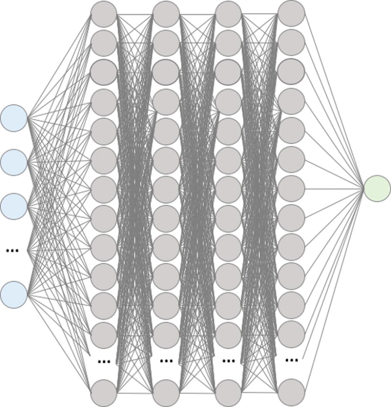
Summary visualization of the deep neural network. Input layer (blue) of features feed into the first hidden layer of 300 neurons with ReLU activations (grey). All the activations of neurons in the first hidden layer are fed into each of the neurons in the second, then all the of the second are fed into the third, and finally all of the third are fed into the fourth. All the activations of the neurons in the fourth hidden layer are then fed into a logistic output layer to produce a probability for in-hospital mortality between 0 and 1.

Model Performance

All performance metrics reported below refer to the test data set (n = 11,997).

i. Area Under the ROC Curves

ROC curves and AUC results are shown in Figure 2 and Table 3. All logistic regression models (LR) and all DNNs had higher AUCs than POSPOM (0.74 (95% CI, 0.68 – 0.79)) and Surgical Apgar (0.58 (95% CI, 0.52 – 0.64)) for predicting in-hospital mortality (Figure 2, Table 3). All DNNs had higher AUCs than LRs for each combination of features except for the reduced feature set with POSPOM (LR 0.90 (95% CI, 0.86 – 0.93) vs DNN 0.90 (95% CI, 0.87 – 0.93)). In addition, reducing the feature set from 87 to 45 features did not reduce the DNN model AUC performance and the addition of ASA and POSPOM as features modestly improved the AUCs of both the full and reduced feature set DNN models. The highest DNN AUC result was the DNN with reduced feature set and ASA (0.91 (95% CI, 0.88 – 0.93)). The highest risk score AUC was RSI (0.97 (95% CI, 0.94 – 0.99)) and the highest LR AUCs were the LR with reduced feature set and ASA (0.90 (95% CI, 0.87 – 0.93)) and the LR with reduced feature set and POSPOM (0.90 (95% CI, 0.86 – 0.93)).

Figure 2.

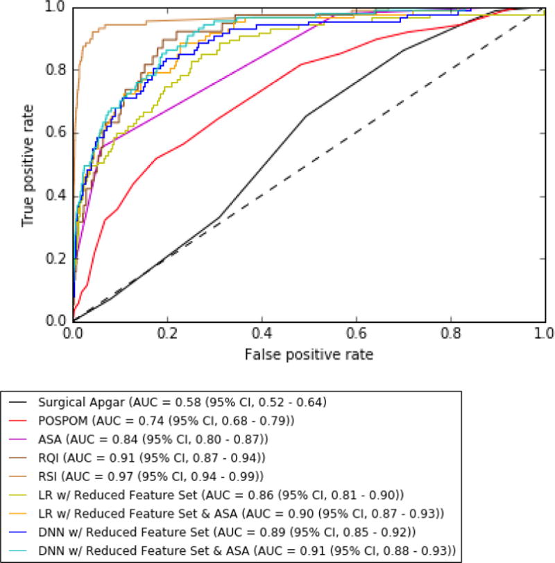
Receiver Operating Characteristic (ROC) Curves to predict postoperative in-hospital mortality

Table 3. Area Under the ROC curve results with 95% confidence intervals for the test set (n = 11,997).

Best AUCs for logistic regression and DNN are in bold.

Clinical Risk Score	AUC (95% CI)
Surgical Apgar	0.58 (0.52 – 0.64)
POSPOM	0.74 (0.68 – 0.79)
ASA	0.84 (0.80 – 0.87)
RQI Score*	0.91 (0.87 – 0.94)
RSI Uncalibrated**	0.97 (0.94 – 0.99)

	AUC (95% CI)
Model	With All 87 features	With ASA (88 features)	With POSPOM (88 features)	With Reduced Feature Set (45 features)	With Reduced Feature Set & ASA (46 features)	With Reduced Feature Set & POSPOM (46 features)
Logistic Regression	0.86 (0.81 – 0.90)	0.89 (0.86 – 0.92)	0.89 (0.85 – 0.93)	0.86 (0.81 – 0.90)	0.90 (0.87 – 0.93)	0.90 (0.86 – 0.93)
DNN	0.88 (0.85 – 0.91)	0.90 (0.87 – 0.93)	0.91 (0.87 – 0.95)	0.89 (0.85 – 0.92)	0.91 (0.88 – 0.93)	0.90 (0.87 – 0.93)

It should be noted that

^*RQI was calculated on 5,591 test patients (38 mortality) and

^**RSI Uncalibrated was calculated on 11,939 test patients (86 mortality)

AUC: Area under the curve; POSPOM: Preoperative Score to Predict Postoperative Mortality; RQI: Risk Quantification Index; RSI: Risk Stratification Index; DNN: Deep neural network.

ii. Choosing a Threshold

For comparison of F1 scores, sensitivity and specificity at different thresholds, DNN with original 87 features (DNN), DNN with a reduced feature set and POSPOM (DNN_rfsPOSPOM), and DNN with a reduced feature set and ASA (DNN_rfsASA) are compared to ASA, POSPOM, logistic regression with original 87 features (LR), logistic regression with a reduced feature set and POSPOM (LR_rfsPOSPOM), and logistic regression with a reduced feature set and ASA (LR_rfsASA) (Table 4). To compare the number of correctly predicted patients by the DNNs at different thresholds, a table of the number of correctly and incorrectly classified patients is shown for all the above models at different thresholds for all test patients (n=11,997) (Table 5).

Table 4.

% of observed mortality patients correctly identified, F1 Score, sensitivity, and specificity performance of ASA; POSPOM; logistic regression model and DNN model with 87 features; logistic regression model and DNN model with reduced feature set and ASA; and logistic regression model and DNN model with reduced feature set and POSPOM at different thresholds. Results for best thresholds chosen by 1) highest % of observed mortality and 2) highest F1 score.

ASA					POSPOM
Threshold	# Obs. Mort. (%)	F1 (95% CI)	Sens. (95% CI)	Spec. (95% CI)	Threshold	# Obs. Mort. (%)	F1 (95% CI)	Sens. (95% CI)	Spec. (95% CI)
3	85 (97.7%)	0.02 (0.02 – 0.03)	0.98 (0.94 – 1)	0.44 (0.43 – 0.45)	10	81 (93.1%)	0.02 (0.01 – 0.02)	0.93 (0.87 – 0.98)	0.23 (0.22 – 0.24)
5	14 (16.1%)	0.24 (0.14 – 0.35)	0.16 (0.09 – 0.25)	1 (1 – 1)	20	31 (35.6%)	0.05 (0.03 – 0.07)	0.36 (0.25 – 0.47)	0.91 (0.90 – 0.91)
Logistic Regression with 87 features					DNN with 87 features
Threshold	# Obs. Mort. (%)	F1 (95% CI)	Sens. (95% CI)	Spec. (95% CI)	Threshold	# Obs. Mort. (%)	F1 (95% CI)	Sens. (95% CI)	Spec. (95% CI)
0.00015	86 (98.9%)	0.01 (0.01 – 0.02)	0.99 (0.96 – 1)	0.003 (0.002 – 0.004)	0.05	86 (98.9%)	0.02 (0.01 – 0.02)	0.99 (0.96 – 1)	0.20 (0.20 -0.21)
0.1	28 (32.2%)	0.24 (0.16 – 0.30)	0.32 (0.22 – 0.42)	0.99 (0.99 – 0.99)	0.3	35 (40.2%)	0.23 (0.17 – 0.30)	0.40 (0.30 – 0.51)	0.99 (0.98 – 0.99)
Logistic Regression with Reduced Feature Set & ASA					DNN with Reduced Feature Set & ASA
Threshold	# Obs. Mort. (%)	F1 (95% CI)	Sens. (95% CI)	Spec. (95% CI)	Threshold	# Obs. Mort. (%)	F1 (95% CI)	Sens. (95% CI)	Spec. (95% CI)
0.0034	84 (96.6%)	0.04 (0.03 – 0.05)	0.97 (0.92 – 1)	0.64 (0.63 – 0.65)	0.22	84 (96.6%)	0.04 (0.03 – 0.05)	0.97 (0.92 – 1)	0.64 (0.64 – 0.65)
0.1	30 (34.5%)	0.26 (0.18 – 0.33)	0.34 (0.24 – 0.44)	0.99 (0.99 – 0.99)	0.4	15 (17.2%)	0.22 (0.12- 0.30)	0.17 (0.09 – 0.25)	1 (1 – 1)
Logistic Regression with Reduced Feature Set & POSPOM					DNN with Reduced Feature Set & POSPOM
Threshold	# Obs. Mort. (%)	F1 (95% CI)	Sens. (95% CI)	Spec. (95% CI)	Threshold	# Obs. Mort. (%)	F1 (95% CI)	Sens. (95% CI)	Spec. (95% CI)
0.002	85 (97.7%)	0.03 (0.02 – 0.03)	0.98 (0.94 – 1)	0.48 (0.48 – 0.49)	0.2	84 (96.6%)	0.04 (0.03 – 0.04)	0.97 (0.92 -1)	0.63 (0.63 – 0.64)
0.1	26 (29.9%)	0.22 (0.15 – 0.29)	0.30 (0.20 – 0.39)	0.99 (0.99 – 0.99)	0.3	40 (46%)	0.18 (0.13 – 0.22)	0.46 (0.36 – 0.56)	0.97 (0.97 – 0.98)

POSPOM: Preoperative Score to Predict Postoperative Mortality; CI: Confidence Interval; DNN: Deep neural network.

Table 5.

The number of correctly and incorrectly classified patients for ASA; POSPOM; logistic regression model and DNN model with 87 features; logistic regression model and DNN model with reduced feature set and ASA; and logistic regression model and DNN model with reduced feature set and POSPOM at different thresholds. Results for best thresholds chosen by 1) highest % of observed mortality and 2) highest F1 score.

ASA					POSPOM
Threshold	# True Negative	# False Positive	# False Negative	# True Positive	Threshold	# True Negative	# False Positive	# False Negative	# True Positive
3	5,244	6,666	2	85	10	2,741	9,169	6	81
5	11,894	16	73	14	20	10,782	1,128	56	31
Logistic Regression with 87 features					DNN with 87 features
Threshold	# True Negative	# False Positive	# False Negative	# True Positive	Threshold	# True Negative	# False Positive	# False Negative	# True Positive
0.00015	37	11,873	1	86	0.05	2,414	9,496	1	86
0.1	11,788	122	59	28	0.3	11,734	176	52	35
Logistic Regression with Reduced Feature Set & ASA					DNN with Reduced Feature Set & ASA
Threshold	# True Negative	# False Positive	# False Negative	# True Positive	Threshold	# True Negative	# False Positive	# False Negative	# True Positive
0.0034	7,578	4,332	3	84	0.22	7,669	4,241	3	84
0.1	11,795	115	57	30	0.4	11,875	35	72	15
Logistic Regression with Reduced Feature Set & POSPOM					DNN with Reduced Feature Set & POSPOM
Threshold	# True Negative	# False Positive	# False Negative	# True Positive	Threshold	# True Negative	# False Positive	# False Negative	# True Positive
0.002	5,772	6,138	2	85	0.2	7,550	4,360	3	84
0.1	11,790	120	61	26	0.4	11,897	12	82	5

POSPOM: Preoperative Score to Predict Postoperative Mortality; DNN: Deep neural network.

If we choose a threshold that optimizes the observed in-hospital mortality rate, the thresholds (% observed mortality) for POSPOM, ASA, and LR, LR_rfsPOSPOM, LR_rfsASA are 10 (93.1%), 3 (97.7%), 0.00015 (98.9%), 0.002 (97.7%), and 0.0034 (96.66%), respectively (Table 4). The thresholds for DNN, DNN_rfsPOSPOM and DNN_rfsASA are 0.05 (98.9%), 0.2 (96.6%) and 0.22 (96.6%), respectively. At these thresholds, POSPOM, ASA, LR, LR_rfsPOSPOM, LR_rfsASA, DNN, DNN_rfsPOSPOM and DNN_rfsASA, all have high and comparable sensitivities. The DNN with the highest AUC DNN_rfsASA had a sensitivity of 0.97 (95% CI, 0.92 – 1) and specificity of 0.64 (95% CI, 0.64 – 0.65) and the LR with the highest AUC LR_rfsASA had a sensitivity of 0.97 (95% CI, 0.92 – 1) and specificity of 0.64 (95% CI, 0.63 – 0.65). However, all DNNs reduced false positives while maintaining the same or similar number of false negatives (Table 5). DNN with all 87 original features decreased the number of false positives compared to LR from 11,873 to 9,169 patients. DNN_rfsASA decreased the number of false positives compared to LR_rfsASA from 4,332 patients to 4,241 patients; and compared to POSPOM and ASA from 9,169 patients and 6,666 patients, respectively.

If we choose a threshold that optimizes precision and recall via the F1 score, the thresholds for POSPOM, ASA, LR, LR_rfsPOSPOM, and LR_rfsASA are higher at 20, 5, 0,1, 0.1, and 0.1, respectively (Table 4). All the thresholds for DNN, DNN_rfsPOSPOM, and DNN_rfsASA also increased to 0.3, 0.4, and 0.3, respectively. The highest F1 scores were comparable for ASA, LR_rfsASA, and DNN_rfsASA at 0.24 (95% CI, 0.14 – 0.35), 0.26 (95% CI, 0.18 – 0.33) and 0.22 (95% CI, 0.12 – 0.30). However, DNN_rfsASA had a lower number of false positives at 35 patients compared to LR_rfsASA 115 patients (Table 5).

iii. Calibration

For comparison of calibration, Brier scores and calibration plots were assessed for LR, DNN_rfsASA, and calibrated DNN_rfsASA. DNN_rfsASA had the worst Brier score of 0.0352, and LR had the best score of 0.0065 (Figure 3). However, the calibrated DNN_rfsASA had a comparable Brier score of 0.0071. Calibration of DNN_rfsASA shifted the best thresholds for observed mortality optimization and F1 optimization from 0.2 and 0.4 to 0.0018 and 0.0048, respectively.

Figure 3.

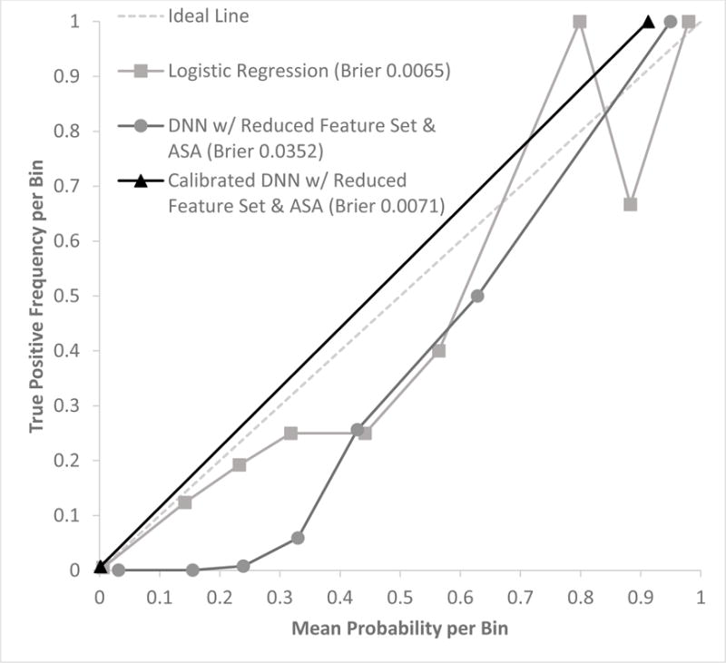
Calibration plot with mean predicted probability vs true positive frequency (# true positives/# samples) per probability value bins in the test data set (n = 11,997) for logistic regression, deep neural network (DNN) with reduced feature set and ASA, and calibrated DNN with reduced feature set and ASA. Bins of predicted probability were at intervals of 0.1: [0 to 0.1), [0.1 to 0.2), …, [0.9 to 1.0).

iv. Feature Importance

To assess feature importance in the DNN, we assessed the decrease in AUC for the removal of groups of features from the best DNN (DNN_rfsasa) (Table 6, Figure 4). For the analysis, 13 groups were used (Age, Anesthesia, ASA, Input, Blood Pressure, Output, Vasopressor, Vasodilator, Labs, Heart Rate, Invasive Line, Inotrope, and Pulse Oximetry). To assess feature importance, we assessed the weights for the logistic regression model (LR_rfsASA) (Figure 5). The top 5 DNN features groups were: labs, ASA, anesthesia, blood pressure, and vasopressor administration. The top LR feature was ASA. In addition, similar to the DNN, vasopressin administration, hemoglobin, presence of arterial or pulmonary arterial line, and sevoflurane administration are found in the top 10 weights.

Table 6.

Table summarizing the features removed with each group during each step of the feature ablation analysis for the DNN. Feature names are defined in Table 1.

Group Type	Feature Removed In Group
Age	AGE
Anesthesia	MAX_ISO
Anesthesia	MAX_SEVO
Anesthesia	MAX_DES
Anesthesia	NITRIC_OXIDE_YN
ASA	ASA_SCORE
Blood Pressure	MAX_DBP
Blood Pressure	MIN_DBP
Blood Pressure	MAX_MAP
Blood Pressure	MIN_MAP
Blood Pressure	MAX_SBP
Blood Pressure	MIN_SBP
Heart Rate	MAX_HR
Heart Rate	MIN_HR
Inotrope	MILRINONE_CURRENT_RATE_MCG_KG_MIN
Inotrope	MILRINONE_MAX_RATE_MCG_KG_MIN
Input	XFUSION_RBC_ML
Input	COLLOID_ML
Input	CRYSTALLOID_ML
Invasive Line	CVC_ANES_YN
Invasive Line	PA_LINE_YN
Invasive Line	ART_LINE_YN
Labs	BASELINE_GFR
Labs	MAX_GLUCOSE
Labs	MIN_GLUCOSE
Labs	MIN_HB
Labs	CURRENT_HB
Labs	STARTING_HB
Output	EBL
Output	UOP
Pulse Oximetry	MAX_PULSE_OX
Pulse Oximetry	MIN_PULSE_OX
Vasodilator	ESMOLOL_CURRENT_RATE_MCG_KG_MIN
Vasodilator	ESMOLOL_MAX_RATE_MCG_KG_MIN
Vasodilator	NICARDIPINE_CURRENT_RATE_MG_HR
Vasodilator	NICARDIPINE_MAX_RATE_MG_HR
Vasodilator	NITROGLYCERIN_CURRENT_RATE_MCG_MIN
Vasodilator	NITROGLYCERIN_MAX_RATE_MCG_MIN
Vasodilator	NITROPRUSSIDE_CURRENT_RATE_MCG_KG_MIN
Vasodilator	NITROPRUSSIDE_MAX_RATE_MCG_KG_MIN
Vasopressor	EPINEPHRINE_CURRENT_RATE_MCG_KG_MIN
Vasopressor	EPINEPHRINE_MAX_RATE_MCG_KG_MIN
Vasopressor	PHENYLEPHRINE_CURRENT_RATE_MCG_MIN
Vasopressor	PHENYLEPHRINE_MAX_RATE_MCG_MIN
Vasopressor	VASO_CURRENT_RATE_UNITS_HR
Vasopressor	VASOPRESSIN_MAX_RATE_UNITS_HR

Figure 4.

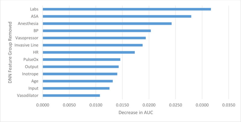
Decrease in AUC performance for each feature group removed during feature ablation analysis for deep neural network with reduced feature set and ASA

Figure 5.

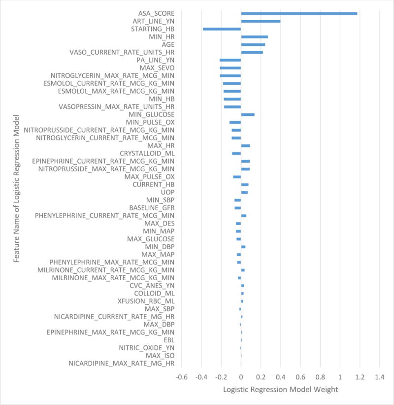
Logistic regression model weight assigned to each feature in the logistic regression model with reduced feature set and ASA.

We have developed a website application that performs predictions for DNN_rfsASA and DNN_rfs on a given data set. The application as well as downloadable model package are available at <risknet.ics.uci.edu>.

Discussion

The results in this study demonstrate that deep neural networks (DNN) can be utilized to predict in-hospital mortality based on automatically extractable and objective intraoperative data. In addition, these predictions are further improved via the addition of preoperative information, as summarized in a patient’s ASA score or POSPOM. The AUC of the “best” DNN model with a reduced feature set and ASA (DNN_rfsASA) also outperformed Surgical Apgar, POSPOM, and ASA. Optimizing thresholds to capture the most observed mortality patients, in other words optimizing for sensitivity, DNN_rfsASA has higher sensitivity than POSPOM, but comparable to ASA, LR_rfsASA, and LR_rfsPOSPOM. This may make sense as ASA is a feature in this DNN model. Most notably, however, is that DNN_rfsASA reduces the number of false positives compared to POSPOM and ASA by 54% and 36%, respectively. DNN_rfsASA also reduced the number of false positives to the most comparably performing logistic regression model LR_rfsASA by 2%. In addition, it should be noted that for each feature set combination (all 87 features, 87 features with ASA, 87 features with POSPOM, reduced features, reduced features with ASA, and reduced features with POSPOM), the DNN slightly outperformed logistic regression, with the exception of the reduced feature set with POSPOM. However, the addition of POSPOM is adding a logistic regression model output as a feature to another logistic regression model, which can be thought of as adding 1 hidden layer to a neural network with a logistic output. While the AUC of logistic regression with the same reduced feature set and ASA (LR_rfsASA) was not significantly lower than DNN_rfsASA, the DNN with all 87 original features outperformed logistic regression with the same 87 features in AUC and significantly decreased the number of false positives by 2,377 patients (20%). This suggests that without careful feature selection to reduce the number of features as well adding preoperative information, logistic regression did not perform comparably to a DNN. Logistic regression can be thought of as a neural network with no hidden layers. When preserving complexity, such as not performing careful feature selection or more rigorous preprocessing, neural networks with many hidden layers are able to perform well and in some cases better than logistic regression.

Due to such a low incidence of true positives (n=87), the numbers for false negatives are hard to compare in this very small mortality population. This small number of mortality patients also affects the interpretation of the calibration results. Extensive data augmentation was used in training the DNN on balanced classes, resulting in predicted probabilities that were shifted up. The DNN’s predicted probability was calibrated to the expected probability of mortality (<1%), and all predicted probabilities were then shifted down well below 0.01 to reflect the % occurrence of in-hospital mortality, while maintaining all performance metrics. After calibration, the calibrated DNN_rfsASA resulted in a better Brier score that was also closer to that of logistic regression, and the optimal mortality threshold for DNN_rfsASA was shifted down from 0.2 to 0.0018, a more reasonable threshold considering the low % occurrence of mortality. For direct comparison in the calibration plot, the same probability bins at intervals of 0.1 were chosen for the DNN_rfsASA calibrated and uncalibrated as well as LR. A limitation of the calibration plot is that it is highly dependent on the choice of bins. This limitation is reflected in the resulting calibration plot for the calibrated DNN_rfsASA, where 86 mortality patients were predicted in the bin [0 to 0.1) and 1 patient was predicted in the bin [0.9 to 1). Thus, the interpretation of these results is limited to the number of true positives that exist.

While the Risk Quantification Index (RQI) had a high and comparable AUC to the DNN_rfsASA, it could only be calculated on 47% of the test patients due to a feature of RQI, specifically the Procedural Severity Score (PSS), which was available for only a limited number of CPT codes. The Risk Stratification Index (RSI) had the highest AUC at 0.97 and unlike RQI, could be calculated on a vast majority of the patients. RSI requires ICD 9 procedural and diagnosis codes. There is are important distinctions to be made between a risk score based on clinical data (ASA, Surgical Apgar, POSPOM, and the logistic regression and DNN models reported here) versus administrative data (RSI, RQI). The first is that present-on-admission diagnoses and planned procedures, i.e. ICD 9 and 10 codes, are theoretically available preoperatively. But in practice, the coding is done after discharge and therefore is not actually available preoperatively to guide clinical care. This makes scores such as RSI appropriate for its intended purpose, comparing hospitals, but not for individual patient care. Finally, point-of-care clinical data contains more information about specific patients than models based only on diagnoses and procedure codes, and therefore should be more specific and useful for guiding the care of individual patients. These distinctions should not be seen as “one is better than another” so much as a matter of selecting the right model for particular purposes.

Perhaps the most attractive feature of this mortality model, is that it provides a fully automated and highly accurate way to estimate the mortality risk of the patient at the end of surgery. All of the data contained in the risk score are easily obtained from the EMR and could be automatically loaded into a model. While the ASA score is subjective, presents with high inter- and intra-rater variability, and does require input from the anesthesiologist into the EMR, this input is common practice as a part of pre-operative assessment. In addition, we have also trained a DNN model using the POSPOM score with comparable performance metrics. Thus, if the clinical need is to be completely objective, the DNN_rfsPOSPOM model would be the most automatic and objective, as POSPOM is based on the presence of key patient co-morbidities and could be automatically obtained from the EMR.

The input into this mortality model is based heavily on intraoperative data available at the end of surgery. There are 45 intraoperative features in the reduced feature set and 1 preoperative feature was added accordingly to leverage preoperative information. The ability of the intraoperative-only mortality models (DNN and DNN with reduced feature set) to maintain high performance with no addition of preoperative features further supports the idea that intraoperative events and management may have a significant effect on post-operative outcomes.

By definition, any screening score will have to tradeoff between sensitivity (capturing all patients with the condition) and specificity (not capturing those who do not have the condition). As a result, clinically, we generally discuss the number needed to treat – the number of “false positives” that must be treated to capture one true positive. Our DNN model not only had the highest AUC, but also reduces the number of false positives – thereby reducing the number needed to treat. Given the current transitions towards value based care, this has some appeal. Another key advantage of a DNN model is its ability to account for the relationships between various clinical factors. For example, in a logistic regression model excess estimated blood loss might be assigned a certain weight and hypotension a different one, thus assigning a linear relationship between hypotension and blood loss. On the other hand, a DNN model could account for the differences and linear or nonlinear associations of hypotension in a minimal blood loss vs significant blood loss case. While a feature could be created to reflect this relationship of hypotension and blood loss and used as an input into a logistic regression model, a DNN model avoids this need for careful feature extraction and is able to create these features on its own. Eventually, integration of DNN models into electronic medical records could result in more accurate risk scores generated automatically per patient, thereby providing real time assistance in the triaging of patients.

Study limitations

There are several limitations to this study. Perhaps most significantly, this study is from a single center and of a somewhat limited sample size. As mentioned above, deep learning models in other fields have included millions of samples. In order to address this limitation and avoid overfitting, we chose a limited number of features and implemented regularization training techniques commonly used in deep learning. In addition, there were only 87 mortality patients in the test data set. Thus, it is possible that the results generated here are not fully generalizable to other institutions and will need to be validated on other data sets.

Conclusion

To the best of our knowledge, this study is the first to demonstrate the ability to use deep learning to predict postoperative in-hospital mortality based on intraoperative EMR data. The deep learning model presented in this study is robust, shows improved or comparable discrimination to other risk scores, and is able to be calculated automatically at the end of surgery and does not rely on any administrative inputs.

Summary Statement.

The results of this study demonstrate that deep neural networks can be utilized to predict in-hospital mortality based on automatically extractable and objective intraoperative data. In addition, these predictions are further improved via the addition of preoperative information, as summarized in a patient’s ASA score or POSPOM. The AUC of the “best” DNN model with a reduced feature set and ASA (DNN_rfsASA) also outperformed Surgical Apgar, POSPOM, ASA, and logistic regression.

References

- 1.Weiser TG, Regenbogen SE, Thompson KD, Haynes AB, Lipsitz SR, Berry WR, Gawande AA. An estimation of the global volume of surgery: a modelling strategy based on available data. The Lancet. 2008;372:139–144. doi: 10.1016/S0140-6736(08)60878-8. [DOI] [PubMed] [Google Scholar]
- 2.Pearse RM, Harrison DA, James P, Watson D, Hinds C, Rhodes A, Grounds MR, Bennett DE. Identification and characterisation of the high-risk surgical population in the United Kingdom. Critical Care. 2006;10:1–6. doi: 10.1186/cc4928. [DOI] [PMC free article] [PubMed] [Google Scholar]
- 3.Pearse RM, Moreno RP, Bauer P, Pelosi P, Metnitz P, Spies C, Vallet B, Vincent J-L, Hoeft A, Rhodes A, Group for the groups of the o, the of Anaesthesiology E Mortality after surgery in Europe: a 7 day cohort study. The Lancet. 2012;380:1059–1065. doi: 10.1016/S0140-6736(12)61148-9. [DOI] [PMC free article] [PubMed] [Google Scholar]
- 4.American Society of Anesthesiologists ASoAASoA. New classification of physical status. Anesthesiology. 1963 [Google Scholar]
- 5.Gawande AA, Kwaan MR, Regenbogen SE, Lipsitz SA, Zinner MJ. An Apgar Score for Surgery. Journal of the American College of Surgeons. 2007;204:201–208. doi: 10.1016/j.jamcollsurg.2006.11.011. [DOI] [PubMed] [Google Scholar]
- 6.Reynolds PQ, Sanders NW, Schildcrout JS, Mercaldo ND, Jacques PJ. Expansion of the Surgical Apgar Score across All Surgical Subspecialties as a Means to Predict Postoperative Mortality. Anesthesiology. 2011;114:1305. doi: 10.1097/ALN.0b013e318219d734. [DOI] [PubMed] [Google Scholar]
- 7.Haynes AB, Regenbogen SE, Weiser TG, Lipsitz SR, Dziekan G, Berry WR, Gawande AA. Surgical outcome measurement for a global patient population: Validation of the Surgical Apgar Score in 8 countries. Surgery. 2011;149:519–524. doi: 10.1016/j.surg.2010.10.019. [DOI] [PubMed] [Google Scholar]
- 8.Regenbogen SE, Ehrenfeld JM, Lipsitz SR, Greenberg CC, Hutter MM, Gawande AA. Utility of the Surgical Apgar Score: Validation in 4119 Patients. Archives of Surgery. 2009;144:30–36. doi: 10.1001/archsurg.2008.504. [DOI] [PubMed] [Google Scholar]
- 9.Terekhov MA, Ehrenfeld JM, Wanderer JP. Preoperative Surgical Risk Predictions Are Not Meaningfully Improved by Including the Surgical Apgar Score. Anesthesiology. 2015;123:1059–1066. doi: 10.1097/ALN.0000000000000858. [DOI] [PubMed] [Google Scholar]
- 10.Manach Y, Collins G, Rodseth R, Bihan-Benjamin C, Biccard B, Riou B, Devereaux PJ, Landais P. Preoperative Score to Predict Postoperative Mortality (POSPOM) Anesthesiology. 2016;124:570–579. doi: 10.1097/ALN.0000000000000972. [DOI] [PubMed] [Google Scholar]
- 11.Schmidhuber J. Neural Networks. Reviews. 2015;61:85–117. doi: 10.1016/j.neunet.2014.09.003. [DOI] [PubMed] [Google Scholar]
- 12.Le Cun Y, Boser B, Denker JS, Henderson D, Howard RE, Hubbard W, Jackel LD. Handwritten Digit Recognition with a Back-Propagation Network. Morgan Kaufmann. 1990 [Google Scholar]
- 13.Baldi P, Chauvin Y. Neural Networks for Fingerprint Recognition. Neural Computation. 1993;5 [Google Scholar]
- 14.Krizhevsky, Sutskever, Hinton E. ImageNet classification with deep convolutional neural networks. Advances in neural information processing systems. 2012 [Google Scholar]
- 15.Szegedy C, Liu W, Jia Y, Sermanet P, Reed S, Anguelov D, Erhan D, Vanhoucke V, Rabinovich A. Going deeper with convolutions. Proceedings of the IEEE Conference on Computer Vision and Pattern Recognition. 2015 [Google Scholar]
- 16.Srivastava K, Greff, Schmidhuber J. Training very deep networks. Advances in Neural Information Processing Systems. 2015 [Google Scholar]
- 17.He K, Zhang X, Ren S, Sun J. Deep Residual Learning for Image Recognition. IEEE Conference on Computer Vision and Pattern Recognition. 2016 [Google Scholar]
- 18.Wu L, Baldi P. Learning to play Go using recursive neural networks. Neural Networks. 2008;21:1392–1400. doi: 10.1016/j.neunet.2008.02.002. [DOI] [PubMed] [Google Scholar]
- 19.Wu L, Baldi P. A scalable machine learning approach to GO. Advances in Neural Information Processing Systems. 2007;19 [Google Scholar]
- 20.Silver D, Huang A, Maddison CJ, Guez A, Sifre L, van den Driessche G, Schrittwieser J, Antonoglou I, Panneershelvam V, Lanctot M, Dieleman S, Grewe D, Nham J, Kalchbrenner N, Sutskever I, Lillicrap T, Leach M, Kavukcuoglu K, Graepel T, Hassabis D. Mastering the game of Go with deep neural networks and tree search. Nature. 2016;529:484–489. doi: 10.1038/nature16961. [DOI] [PubMed] [Google Scholar]
- 21.Baldi P, Sadowski P, Whiteson D. Searching for exotic particles in high-energy physics with deep learning. Nature Communications. 2014;5 doi: 10.1038/ncomms5308. [DOI] [PubMed] [Google Scholar]
- 22.Sadowski PJ, Collado J, Whiteson D, Baldi P. Deep Learning, Dark Knowledge, and Dark Matter. Journal of Machine Learning Research, Workshop and Conference Proceedings. 2015;42 [Google Scholar]
- 23.Kayala MA, Azencott C-A, Chen JH, Baldi P. Learning to Predict Chemical Reactions. Journal of Chemical Information and Modeling. 2011;51:2209–2222. doi: 10.1021/ci200207y. [DOI] [PMC free article] [PubMed] [Google Scholar]
- 24.Kayala MA, Baldi P. ReactionPredictor: Prediction of Complex Chemical Reactions at the Mechanistic Level Using Machine Learning. Journal of Chemical Information and Modeling. 2012;52:2526–2540. doi: 10.1021/ci3003039. [DOI] [PubMed] [Google Scholar]
- 25.Lusci A, Pollastri G, Baldi P. Deep Architectures and Deep Learning in Chemoinformatics: The Prediction of Aqueous Solubility for Drug-Like Molecules. Journal of Chemical Information and Modeling. 2013;53:1563–1575. doi: 10.1021/ci400187y. [DOI] [PMC free article] [PubMed] [Google Scholar]
- 26.Lena P, Nagata K, Baldi P. Deep architectures for protein contact map prediction. Bioinformatics. 2012;28:2449–2457. doi: 10.1093/bioinformatics/bts475. [DOI] [PMC free article] [PubMed] [Google Scholar]
- 27.Baldi P, Pollastri G. The principled design of large-scale recursive neural network architectures–dag-rnns and the protein structure prediction problem. Journal of Machine Learning Research. 2003;4 [Google Scholar]
- 28.Zhou J, Troyanskaya OG. Predicting effects of noncoding variants with deep learning-based sequence model. Nature Methods. 2015;12:931–934. doi: 10.1038/nmeth.3547. [DOI] [PMC free article] [PubMed] [Google Scholar]
- 29.Guillame-Bert M, Dubrawski A, Wang D, Hravnak M, Clermont G, Pinsky MR. Learning temporal rules to forecast instability in continuously monitored patients. Journal of the American Medical Informatics Association: JAMIA. 2016;24:47–53. doi: 10.1093/jamia/ocw048. [DOI] [PMC free article] [PubMed] [Google Scholar]
- 30.Chen L, Dubrawski A, Clermont G, Hravnak M, Pinsky M. Modelling Risk of Cardio-Respiratory Instability as a Heterogeneous Process. AMIA Annual Symposium Proceedings. 2015 [PMC free article] [PubMed] [Google Scholar]
- 31.Frizzell JD, Liang L, Schulte PJ, Yancy CW, Heidenreich PA, Hernandez AF, Bhatt DL, Fonarow GC, Laskey WK. Prediction of 30-Day All-Cause Readmissions in Patients Hospitalized for Heart Failure: Comparison of Machine Learning and Other Statistical Approaches. JAMA Cardiology. 2016 doi: 10.1001/jamacardio.2016.3956. [DOI] [PubMed] [Google Scholar]
- 32.Shadmi E, Flaks-Manov N, Hoshen M, Goldman O, Bitterman H, Balicer RD. Predicting 30-Day Readmissions With Preadmission Electronic Health Record Data. Medical Care. 2015;53:283. doi: 10.1097/MLR.0000000000000315. [DOI] [PubMed] [Google Scholar]
- 33.Nguyen, Tran, Wickramasinghe Deepr: A Convolutional Net for Medical Records. doi: 10.1109/JBHI.2016.2633963. arXiv 2016; 1607.07519v1. [DOI] [PubMed] [Google Scholar]
- 34.Lipton Z, Kale D, Elkan C, Wetzel R. Learning to Diagnose with LSTM Recurrent Neural Networks. International Conference on Learning Representations. 2016 [Google Scholar]
- 35.Razavian N, Sontag D. TEMPORAL CONVOLUTIONAL NEURAL NETWORKS FOR DIAGNOSIS FROM LAB TESTS. arXiv 2016; 1511.07938v4. [Google Scholar]
- 36.Gulshan V, Peng L, Coram M, Stumpe MC, Wu D, Narayanaswamy A, Venugopalan S, Widner K, Madams T, Cuadros J, Kim R, Raman R, Nelson PC, Mega JL, Webster DR. Development and Validation of a Deep Learning Algorithm for Detection of Diabetic Retinopathy in Retinal Fundus Photographs. JAMA. 2016;316:2402–2410. doi: 10.1001/jama.2016.17216. [DOI] [PubMed] [Google Scholar]
- 37.Luo W, Phung D, Tran T, Gupta S, Rana S, Karmakar C, Shilton A, Yearwood J, Dimitrova N, Ho TB, Venkatesh S, Berk M. Guidelines for Developing and Reporting Machine Learning Predictive Models in Biomedical Research: A Multidisciplinary View. J Med Internet Res. 2016;18:e323. doi: 10.2196/jmir.5870. [DOI] [PMC free article] [PubMed] [Google Scholar]
- 38.Hofer IS, Gabel E, Pfeffer M, Mahbouba M, Mahajan A. A Systematic Approach to Creation of a Perioperative Data Warehouse. Anesth Analg. 2016;122:1880–4. doi: 10.1213/ANE.0000000000001201. [DOI] [PubMed] [Google Scholar]
- 39.Baldi P, Sadowski P. The dropout learning algorithm. Artificial Intelligence. 2014;210:78–122. doi: 10.1016/j.artint.2014.02.004. [DOI] [PMC free article] [PubMed] [Google Scholar]
- 40.Srivastava N. Dropout: A Simple Way to Prevent Neural Networks from Overfitting. Journal of Machine Learning Research. 2014;15 [Google Scholar]
- 41.Hinton GE, Srivastava N, Krizhevsky A. Improving neural networks by preventing co-adaptation of feature detectors. 2012 arXiv:1207.0580. [Google Scholar]
- 42.Sigakis MJG, Bittner EA, Wanderer JP. Validation of a Risk Stratification Index and Risk Quantification Index for Predicting Patient Outcomes: In-hospital Mortality, 30-day Mortality, 1-year Mortality, and Length-of-stay. Anesthesiology. 2013;119:525. doi: 10.1097/ALN.0b013e31829ce6e6. [DOI] [PubMed] [Google Scholar]
- 43.Sessler DI, Sigl JC, Manberg PJ, Kelley SD, Schubert A, Chamoun NG. Broadly Applicable Risk Stratification System for Predicting Duration of Hospitalization and Mortality. Anesthesiology. 2010;113:1026. doi: 10.1097/ALN.0b013e3181f79a8d. [DOI] [PubMed] [Google Scholar]
- 44.Chollet F. Keras. 2015 < https://github.com/fchollet/keras>. GitHub.
- 45.Pedregosa F, Varoquaux G, Gramfort A, Michel V, Thirion B, Grisel O, Blondel M, Prettenhofer P, Weiss R, Dubourg V. Scikit-learn: Machine learning in Python. Journal of Machine Learning Research. 2011;12 [Google Scholar]
Associated Data
This section collects any data citations, data availability statements, or supplementary materials included in this article.