

Abstract
Accurate segmentation of specific organ from computed tomography (CT) scans is a basic and crucial task for accurate diagnosis and treatment. To avoid time-consuming manual optimization and to help physicians distinguish diseases, an automatic organ segmentation framework is presented. The framework utilized convolution neural networks (CNN) to classify pixels. To reduce the redundant inputs, the simple linear iterative clustering (SLIC) of super-pixels and the support vector machine (SVM) classifier are introduced. To establish the perfect boundary of organs in one-pixel-level, the pixels need to be classified step-by-step. First, the SLIC is used to cut an image into grids and extract respective digital signatures. Next, the signature is classified by the SVM, and the rough edges are acquired. Finally, a precise boundary is obtained by the CNN, which is based on patches around each pixel-point. The framework is applied to abdominal CT scans of livers and high-resolution computed tomography (HRCT) scans of lungs. The experimental CT scans are derived from two public datasets (Sliver 07 and a Chinese local dataset). Experimental results show that the proposed method can precisely and efficiently detect the organs. This method consumes 38 s/slice for liver segmentation. The Dice coefficient of the liver segmentation results reaches to 97.43%. For lung segmentation, the Dice coefficient is 97.93%. This finding demonstrates that the proposed framework is a favorable method for lung segmentation of HRCT scans.
Keywords: Organ segmentation, Super-pixels, CNN, SVM classifier, CT scans
Introduction
CT is one of the most significant medical imaging technologies to assess the human body. Human CT scans contain abundant information, such as complex soft-tissues and vascular and multiple organs, including the liver, kidney, gallbladder, lung, and spleen. For computer-aided diagnosis, segmentation for the region of interest (ROI) in CT images is a key precondition. Therefore, seeking a generic method that can replace manual segmentation is urgent.
Several state-of-the-art algorithms, including thresholding, region-based methods, and graph cut, have been proposed to assist organ segmentation. Thresholding is one of the simplest and the most classical methods for segmenting images that are light objects on dark backgrounds. For example, Moltz [1] combined a threshold-based approach with morphological processing and achieved the accurate segmentation of liver tumors. Compared with other strategies, thresholding involved fewer calculations, but it does not account for the spatial characteristics, since it is sensitive to noise.
Region growing [2] is a typical application of region-based methods. This application is a procedure that clusters all the pixels into sub-regions according to a predefined criterion. For example, Devi K G [3] used a 3D regional growth method to distinguish between the kidneys, spleen, and three other organs. However, region growing is a method that depends on the seed region selection. Researchers usually select the seed points to improve the quality of segmentation. An adaptive regional growth method that learns the homogenous criteria from characteristics of the region was presented by [4]. However, the efficiency depends on the homogeneity of the tissue. Under-segmentation will occur when the target is inhomogeneous.
The core of graph cuts represents the image to an undirected weighted graph. Oda M [5] applied graph cut to four-organ segmentation. Graph cut is not always automatic, since it needs users to carefully select seed points labeled as the “object” and “background” [6].
Several machine learning-based attempts [7–9] have also been applied to the domain. Existing work in multi-organs segmentation can be roughly divided into registration-based and classification-based methods [10]. Several classification-based methods [11–13] used traditional classifiers to extract appearance features. Researchers in the field of medical imaging investigate the potential of deep learning in medical images acquired with CT, MRI, and PET [14]. Deep learning (DL) has shown promising accuracy as an automatic segmentation algorithm. Meanwhile, certain specific DL frameworks are primarily being performed for classification [15–17], objects detection (lesions, organs) [18–21], and segmentation [22, 23]. CNN [24] is an effective branch of deep artificial neural networks. Kayalibay [25] achieved effective segmentation of hand and brain MRIs using the CNN-based method. Employing a similar approach, Cha K [26] segmented the bladder, and Zou Y [27] segmented several digestive organs.
In CNN-based semantic segmentation tasks, the patch-based method transforms segmentation into pixel-wise classification. The strategy improved segmentation with more precise outputs. However, in spite of the high classification accuracy, the traditional CNN cannot avoid poor results, which caused by huge input data. In other words, reducing data redundancy can promote segmentation. A novel CNN framework that provides substantial improvements using super-pixels and a support vector machines (SVM) is presented in this paper.
Abdominal CTs can reflect multiple organs; however, abdominal CTs can image only a part of the lung bases, and they cannot be used to detect most lung diseases due to the incomplete reflection. At present, a most common clinical tactic to detect lung disease is HRCT. HRCT enhances parameters to maximize the spatial resolution at the time of imaging. HRCT can clearly reflect lung tissue and is regarded as the first option for the diagnosis of pulmonary diffuse lesions.
For the two types of CT images, we emphasize determining the contours and then extracting entire regions of organs. The presented framework was verified using liver and lung segmentation with desirable outputs.
The next section provides details of the dataset and methods. The section after that describes the experimental results and the evaluation. Finally, we discuss and conclude the results.
Materials and Methods
Experimental Environment
The whole experiment was performed on a PC with Linux Ubuntu 14.04 LST 64-bit operating system with an Intel i3 3.6 GHz CPU (Intel Core i3-4160), 16 GB of memory and an NVIDIA GeForce GTX 960 graphics card. The CNN was trained and tested using the CAFFE deep learning library [28]. The algorithms (including the super-pixel and post-processes) are conducted on MATLAB 2016a software. Since LIBSVM is one of the most widely used SVM libraries of [29], the involved SVM classifier is based on LIBSVM 3.14.
Materials
The experimental data are comprised of two parts: the liver dataset and the lung dataset.
The liver data comes from the public dataset Sliver 07 [30]. The dataset consists of abdominal CT scans from 20 anesthetized patients (more than 5500 liver slices) and regional annotations. The CT scans are in grayscale with 512 × 512 pixels.
The lung data are gathered from the open Chinese dataset TIANCHI Medical AI Challenge [31]. The dataset is composed of 13 HRCT scans. The sum of CT images reaches to 5000 slices, and the CT slices are all in grayscale with 512 × 512 pixels. The corresponding ground truths of all lung slices are marked by a specific group of 4 radiologists. The radiologists are all clinicians working at the First Hospital of Jilin University, China, and their experience levels are detailed as follows: Radiologist1 is a chief physician with 24 years of experience. Radiologist2 is an attending doctor with 13 years of experience. Radiologist3 is an attending doctor with 6 years of experience. Finally, Radiologist4 is a physician with 3 years of experience. The process of annotation is divided into two steps. In the initial blinded-read phase, each radiologist independently reviewed each CT slice and marked the lung region. In the subsequent unblinded-read phase, each radiologist independently reviewed their own marks along with the anonymous marks of the three other radiologists to render a final opinion.
Finally, we processed the two dataset via the “leave-one-patient-out” cross-validation tactic to divide the original dataset into a training set and a testing set.
Methods
We intend to classify each pixel of the CT images via CNN. To reduce the input, the super-pixel and SVM classifier are introduced. Organ segmentation is executed in following manner. First, CT slices are decomposed into a set of disjointed super-pixels by the SLIC. Next, calculation is performed on each super-pixel region and a multi-elemental array is formed. The digital signature of the array contains divided mathematical criteria of the SLIC. These signatures represent the characteristics of different organs in abdominal CT images. Even if the selected organ is by itself, more information can be obtained from the figures. Compared to the ground truth, the selected super-pixels are divided into three parts: all-organ area (labeled as 1), mixed area (labeled as 0), and non-organ area (labeled as − 1). Then, ample labeled vectors are put into SVM classifier to train a model. Through the trained SVM model, all super-pixel blocks in the CT images could be automatically classified. The SVM reduces the computational efforts and identifies the initial liver boundary [32].
Consequently, we utilize the CNN to refine the rough edges. We treat a single pixel on an edge as the center and cut a specific sized patch around it. Next, the patches are fed into CNN, and a training model is obtained. The CNN model can achieve pixel-wise assorting and smooth the rough edges. To date, the desirable contours of organs in CT images have already been extracted through above procedure. Finally, the output from the CNN is post-processed. In this phase, several kinds of morphological treatments are manipulated to complete the outputs. Certain interrupted edges are connected by close operation. Next, the closed areas are filled. The erosion operation is employed to eliminate thin protrusions and tiny isolated areas to obtain the final results. The above master steps can be viewed in the flow diagram in Fig. 1.
Fig. 1.

Flow diagram of the main steps
SLIC
Within a super-pixel, pixels have similar colors, textures, and intensities [33]. SLIC [34] has been proven as a fast and effective method to generate super-pixels. SLIC proceeds in the following steps.
-
Step 1.
Initializing the seed points. The sole parameter of the SLIC algorithm is K, which indicates the desired amount of the equally sized super-pixels. Assuming that the image includes a total of N pixels, then the size of each super-pixel grid is N/K. The approximate size of grids is
| 1 |
-
Step 2.
Assignment. Once each pixel i is related to the nearest cluster center; there is a step to update the center by adjusting the mean [l,a,b,x,y]T vector, where l means light, and a and b represent the color changing trends. In the CIELAB color space, the information involving color is represented by the vector [l,a,b]T, while the pixel’s position is located by the vector [x,y]T.
-
Step 3.
Distance measurement. According to the presented vector, it is necessary to normalize color proximity and spatial proximity using the formulas
| 2 |
| 3 |
To combine the two distances into a single measure, the formula is defined as
| 4 |
where S represents the interval between grids, and m is the balanced parameter used to weigh the proportions of color information and spatial information in this measurement. Finally, a separate number was assigned to each cluster on the basis of the computed distance.
-
Step 4.
Connection. Disjointed pixels were redistributed to nearby super-pixels to enhance the connectivity.
Figure 2b shows the segmentation result when the parameter K equals 200. Super-pixel grids can be divided into three categories: all-organ areas (labeled as 1), non-organ areas (labeled as − 1), and mixed areas (labeled as 0). Figure 2b exhibits the label assignment.
Fig. 2.

a Original image. b Illustration image with labeled super-pixel when K = 200
In the CIELAB color space, the pixels in the same super-pixel grid share similar digital signatures including color and spatial information, which are represented by a mean vector [l,a,b,x,y]T. However, in grayscale images, the expression of [l,a,b]T would be invalid. We employ the mean and variance of grayscale values in each super-pixel grid to indicate the fluctuation of grayscale color. Therefore, the mathematical trait is re-denoted by the vector [x,y,m,v]T, in which m and v are the mean and variance respectively.
The selection of the parameter K can be pivotal, since it directly determines the number of vectors. A small size cannot provide a sufficient signature, and an overly large size will increase complexity and cause over-fitting. With respect to the accuracy of the SVM on the liver dataset, we assess it with a K range of 200–2000 with an interval of 200. The accuracy trend is shown in Fig. 3. We notice that the accuracy steadily increases between K = 200 and K = 1000, and then slightly fluctuates from K = 1200 to K = 2000. Therefore, we carry out another detailed comparison from K = 1200 to K = 2000 with an interval of 100. The second accuracy trend is displayed in Fig. 4. It is obvious that the optimal selection is when K = 1500. An exemplary output of SLIC is shown in Fig. 5.
Fig. 3.

Rough line chart of selection of K
Fig. 4.

Detailed line chart of the selection of K
Fig. 5.

a Liver segmentation result of SLIC when K = 1500. b Lung segmentation result of SLIC when K = 1500
SVM Classifier
SVM is a statistically robust learning method based on structural risk minimization [35]. When solving small-sample, non-linear, and multi-dimensional data in our experiment, the SVM classifier displays unique advantages.
As the name implies, the SVM classifier demands vectors. The extracted features adapt to this requirement. The target of the SVM is to find an optimal solution to the hyper-plane and separate the data among 3 classes (1, 0, and − 1). Each training data instance consists of a (pi, qi) pair, and we defined the pair as
| 5 |
| 6 |
where i represents the i-th vector, and N is the total number of vectors.
For the given pairs, selecting the appropriate parameters for LIBSVM would directly affects the accuracy. First, parameter s = 0 represents the classification mode. Since the scale of the extracted features is not large, it is unnecessary to reflect the limited features to a high dimensional space. Therefore, the kernel function is set to RBF and parameter t is 2. Parameter v = n represents the n-fold cross-validation tactic and we adopt v = n = 10. For classification, the four elements play equal roles so that w = 1.
Otherwise, the precision depends on the site of gamma (parameter g) and cost (parameter c). To locate the appropriate parameters of c and g, a piece of brief code about parameter optimization is introduced. The details are exhibited in Algorithm 1.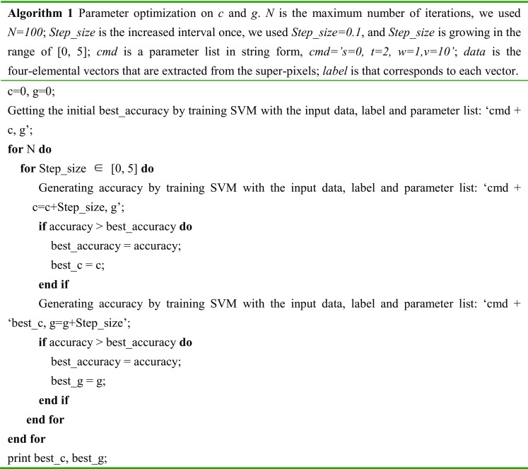
Algorithm 1 realizes the best accuracy when g = 1.2, c = 2.7.
Using the optimal combination of selected parameters, the SVM separates the super-pixels of the testing scans into 3 classes: all-organ area (labeled as 1), mixed area (labeled as 0), and non-organ area (labeled as − 1). Finally, among the target of edges collection, only the grids labeled as 0 are reserved for the further refinement.
CNN
CNN is a popular branch of deep learning. In 2012, Alex Krizhevsky [36] proposed a classical CNN model, which was called AlexNet by the scholars in this field.
AlexNet consists of five convolutional layers (Conv1~Conv5), three max-pooling layers (Pool1, Pool2, and Pool5) and three fully connected layers (Fc1–Fc3). We adopt the original structure, loss function, optimizer, and most parameters except for the num-output of the traditional AlexNet. The parameter num-output represents the numbers in each layer. Num-output should be adjusted so that the model can be better adapted to the input. The details of the resetting are shown in Table 1, and the revised structure is exhibited in Fig. 6.
Table 1.
Parameters of the proposed CNN
| Layer | Kernel | Stride | Pad | Output size |
|---|---|---|---|---|
| Data | – | – | – | 99 × 99 |
| Conv1 | 11 | 4 | 0 | 23 × 23 × 64 |
| Pool1 | 8 | 1 | 0 | 16 × 16 × 64 |
| Conv2 | 5 | 1 | 2 | 16 × 16 × 128 |
| Pool2 | 4 | 2 | 0 | 7 × 7 × 128 |
| Conv3 | 3 | 1 | 1 | 7 × 7 × 256 |
| Conv4 | 3 | 1 | 0 | 5 × 5 × 256 |
| Conv5 | 3 | 1 | 1 | 5 × 5 × 200 |
| Pool5 | 3 | 2 | 0 | 2 × 2 × 200 |
| Fc1 | – | – | – | 2 × 2 × 128 |
| Fc2 | – | – | – | 2 × 2 × 32 |
| Fc3 | – | – | – | 2 × 2 × 2 |
Fig. 6.

Structure of the proposed CNN
To improve the performance of the architecture, we need to collect a large amount of pixels to make it more powerful and intelligent. Therefore, splitting out patches of the detected edges is an ideal solution. The AlexNet captures information from patches, simplifies the sources, and exports feature maps layer by layer. The size of a patch directly influences the “receive filed” of the aftermost feature map.
In the framework of CAFFE, the length of the “receive filed” in each layer can be calculated as
| 7 |
For the input of 512 × 512 pixels, each super-pixel contains approximately 175 pixels when K = 1500. Since the CNN is performed based on super-pixels, the final “receive filed” should be smaller than the average area of the super-pixels. In other words, the maximum of the length is pixels. The other correspondence can be found in Table 2.
Table 2.
Correspondence between the size of patch and the area of final “receive filed”
| The size of patch (pixels) | The area of receive filed (pixels2) | The size of patch (pixels) | The area of receive filed (pixels2) | The size of patch (pixels) | The area of receive filed (pixels2) |
|---|---|---|---|---|---|
| 275 | 13 × 13 | 195 | 8 × 8 | 115 | 3 × 3 |
| 259 | 12 × 12 | 179 | 7 × 7 | 99 | 2 × 2 |
| 243 | 11 × 11 | 163 | 6 × 6 | 83 | 1 × 1 |
| 227 | 10 × 10 | 147 | 5 × 5 | ||
| 211 | 9 × 9 | 131 | 4 × 4 | – | – |
With respect to the accuracy of CNN on the liver dataset, we try every sized of patch mentioned in Table 2. The accuracy is shown in Fig. 7.
Fig. 7.

Line chart of the selection of the patch size
After repeated experiments, the patches whose size is 99 pixels are located at the highest rate of accuracy. The square patches are cut from the original CT images with a size of 99 × 99 pixels2. It is a reasonable size, since there need to be enough big regions for the CNN to distinguish boundaries and ensure it is the target boundary. These patches are centered at every point on the boundary, which is selected by the mixed super-pixels in the section Materials and Methods-SVM. Some patches are given in Fig. 8.
Fig. 8.

a–e Illustrations of extracted patches
We used an untrained CNN with the above structure of AlexNet structure. The patches are trained on CAFFE with randomly initial weights. Based on the trained model, the points on the rough boundary are sorted into two kinds: points of organ region (labeled as 1) or points of background region (labeled as 0). When all the organ regions are maintained, smooth edges are effectively obtained.
Post-process
The presented segmentation method is emphasized on contour extracted. However, there are some flaws in the obtained boundary, including slight interruption and tiny errors in predicted regions, as shown in Fig. 9. Therefore, we applied some morphological operations to correct for the deviation.
Fig. 9.

An example of the flaws
The open operation is used to remove isolated regions, and the close operation is used to connect breakpoints on the border. Finally, we acquire closure on the contour. Then, the inner area is filled and the segmentation result is obtained (Fig. 10d).
Fig. 10.

a Original image, b rough liver boundary from SVM, c liver boundary from CNN, d liver segmentation result from the presented framework, e liver segmentation result from patch-based CNN only, and f liver ground-truth image
Evaluation Metrics
Dice’s similarity coefficient [37] can directly reflect the similarity between the segmentation result and the ground truth. It is considered as a most common metric when evaluating the accuracy of the segmentation algorithm. It can be calculated as
| 8 |
Evaluation Metrics on Liver Dataset
The mean Dice of the final results reaches to 97.43% on the liver dataset.
However, in order to highlight different aspects of segmentation quality and acquire a comprehensive assessment, a variety of different measures should be employed. According to the literature [38], a scoring system is proposed for liver segmentation.
The score is defined as
| 9 |
| 10 |
where ϕ represents final score, ϕi is the score computed for each individual output slice, εi is the actual value of the corresponding metric for each output slice, and is the mean of all outputs.
The described scoring system was employed with the following five error measures: volumetric overlap error (VOE) [39], relative volume difference (RVD), average symmetric surface distance (ASD), maximum symmetric surface distance (MSD), and root mean square symmetric surface distance (RMSD). Theses metrics are defined by the expressions
| 11 |
| 12 |
| 13 |
| 14 |
| 15 |
where A represents the segmentation results, and B represents the ground truth. B1 represents the boundary of the result, B2 represents the boundary of the ground truth, S(A) represents the area of the resulting image, and S(B) represents the area of the ground truth.
Among these metrics, VOE is 0 for a perfect segmentation and 1 if segmentation and reference do not overlap at all. RVD reveals whether a method tends to over-segment or under-segment, where a value of 0 means that both volumes are identical. RMSD is sensitive to outliers and returns the true maximum error. For RMSD, ASD, and MSD, 0 represents a perfect segmentation.
Results
Result on Liver Dataset
The accuracy of the SVM is enhanced by the parameter adjustment in Table 3.
Table 3.
Parameters setting of LIBSVM
| Parameters | s | t | g | c | w | v |
|---|---|---|---|---|---|---|
| Value | 0 | 2 | 1.2 | 2.7 | 1 | 10 |
The accuracy of the SVM classifier on the liver testing set reaches 93.41 ± 0.59%. The accuracy of CNN is 89.33 ± 1.12%. An example of the results is shown in Fig. 10.
From Fig. 10, it is intuitive to observe that the results are very close to the true case. The results show that the pre-processing of the super-pixel and SVM promotes segmentation. Figure 10e is an output of the same CNN model, but the testing patches are cut from all pixels of the original CT image. Though accuracy of the trained CNN does not change, the false predictions are increased actually with the large-scale input. The comparison demonstrates that the pre-processing effectively reduces input redundancy.
Result on Lung Dataset
The accuracy of the SVM classifier on the lung testing set is 92.9 ± 0.83%. The accuracy of the CNN reaches 91.8 ± 1.37%. An example of the results of lung segmentation is shown in Fig. 11.
Fig. 11.

a Original image, b rough lung boundary from SVM, c lung boundary from CNN, d lung segmentation result from the presented framework, and e lung ground-truth image
From the lung segmentation result of Fig. 11, we can conclude that the presented framework can maintain the integral and symmetrical of the segmentation for both the left lung and the right lung.
Evaluation
Evaluation on Liver Dataset
For the same datasets, the proposed framework is comparable to the state-of-art methods. Table 4 displays a further comparison among the other methods.
Table 4.
Liver segmentation results comparison
| Method | Runtime (s/slice) | VOE (%) | RVD (mm) | ASD (mm) | MSD (mm) | RMSD (mm) | Score | |
|---|---|---|---|---|---|---|---|---|
| Ref. [40] | 135 | 5.35 | − 0.17 | 0.84 | 19.58 | 1.78 | 80.3 | |
| Ref. [41] | 90 | 5.42 | 1.75 | 0.79 | 33.55 | 1.87 | 76.2 | |
| Ref. [42] | 285 | 6.24 | 1.18 | 1.03 | 18.82 | 2.11 | 77.9 | |
| Ref. [43] | 120–180 | 4.58 | 1.08 | 0.68 | 16.88 | 1.45 | 83.4 | |
| Ref. [44] | 27 | 7.87 | 1.31 | 1.29 | 23.56 | 2.50 | 71.4 | |
| Ref. [45] | 24–184 | 5.90 | 2.70 | 0.91 | 18.94 | 1.88 | 77.8 | |
| Ours | 38 | 6.17 | 1.33 | 1.48 | 17.80 | 2.19 | 78.1 |
The above methods were all performed using the same dataset as ours. [40, 41, 45] adopted traditional methods. [42–44] proposed methods based on DL. Table 3 summarizes that the presented framework is better with lower time consumption. Compared to [44, 45], the proposed method improves accuracy. Compared to [40–43], in the case of similar scores, the proposed method reduces the processing time.
To test the segmentation performance for different liver shapes, we divide the testing set into 10 subsets. Each subset shares a similar form or liver size. The scale of each subset is unequal, and the number of slices ranges from 87 to 411. Instances of liver regions in some subsets are shown in Fig. 12. Table 4 records the performances in subsets 1–10.
Fig. 12.

a An example slice with the ground truth in subset 2, b an example slice with the ground truth in subset 3, c an example slice with the ground truth in subset 6, and d an example slice with the ground truth in subset 7
In Table 5, the average areas liver is a metric used to measure the relative liver size of different subsets. Table 5 also shows the fluctuation of the six measurements by average and variance. The value of mean Dice is 97.1%, with the other five metrics being reasonable. It reveals that the method is steady and can well adapt to various liver forms.
Table 5.
Results for livers of different sizes
| Number | Average liver areas (pixels/slice) | Dice (%) | VOE (%) | RVD (%) | ASD (mm) | MSD (mm) | RMSD (mm) |
|---|---|---|---|---|---|---|---|
| 1 | 10,137 | 96.5 | 6.61 | − 2.48 | 1.40 | 17.34 | 2.55 |
| 2 | 13,071 | 96.2 | 6.67 | − 1.25 | 1.19 | 16.21 | 2.37 |
| 3 | 22,672 | 97.9 | 5.93 | 2.00 | 1.04 | 16.29 | 2.21 |
| 4 | 22,955 | 98.3 | 5.68 | − 0.72 | 1.13 | 15.67 | 2.14 |
| 5 | 26,685 | 96.8 | 6.31 | 1.78 | 1.06 | 16.99 | 2.48 |
| 6 | 33,017 | 97.3 | 5.97 | − 1.89 | 1.22 | 16.45 | 2.25 |
| 7 | 47,535 | 98.2 | 5.03 | 1.33 | 0.71 | 15.93 | 1.89 |
| 8 | 47,860 | 96.3 | 6.86 | 1.79 | 1.47 | 16.19 | 2.37 |
| 9 | 49,533 | 96.9 | 6.02 | − 1.38 | 1.15 | 16.71 | 2.41 |
| 10 | 55,095 | 97.0 | 5.21 | 1.13 | 1.27 | 16.24 | 1.99 |
| Average Variance |
– – |
97.1 0.76 |
6.03 0.61 |
0.03 1.73 |
1.16 0.21 |
16.40 0.49 |
2.27 0.21 |
Evaluation on Lung Dataset
We applied a novel segmentation framework on a lung dataset. According to formula (8), the mean Dice of the final results reaches 97.93%. Processing a slice requires 40 s.
Most existing studies on lung segmentation are performed on local datasets. To avoid unfair comparisons, we provide with a rough contrast [46] and [47] adopt traditional methods. The mean Dice of [46] is 98.62%, and the mean Dice of [47] is 93.7% [48] proposes a method based on DL and obtains a mean Dice of 98.5%. From there results, we can conclude that the presented framework works well on both abdominal CTs and HRCTs.
Discussion
In clinical applications, automatic segmentation methods that can detect multiple targets would be convenient for medical staff and benefit patients. The presented framework is accomplished-based liver and lung segmentations from CT scans.
We verified the framework on two different CT forms, the abdominal CT and the HRCT. In abdominal CT images, the discrimination between the liver and surrounding tissues are usually unclear due to low resolution, and the shapes and locations of livers are not always regular. Nonetheless, the HRCT is a CT imaging method with enhanced resolution. The desirable output of our method is a testimony to the flexibility for both high and low resolutions. In procedure of liver segmentation, the Dice coefficient reaches 97.43%. Table 4 demonstrates that the performance of the presented framework is comparable to other single-purpose methods. For the exploration of segmentation performances for different liver shapes, Table 5 proves that our method is robust.
We also made an attempt to segment lungs for HRCT using the proposed framework. All related parameter settings are the same with liver segmentation. The mean Dice of the final results reaches 97.93%. From the output shown in Fig. 11d, the morphology of the obtained lungs is complete and symmetrical. A precise and efficient method of lung segmentation is significant to the diagnosis of pectoral disease. Lung segmentation is a crucial first step for the consequential detection of many pectoral diseases, such as pulmonary nodules and diffuse pneumonia, and the method can play a role in this regard. All the parameters in the presented framework are adjusted on the liver dataset. We except to fine-tune the framework and make it more fitting to the lung segmentation in the future. It could contribute to the higher accuracy on lung segmentation.
In addition, the structure of DL determines the running time reduction. The time consumed by the liver segmentation is 38 s/slice. For the left and right lungs segmentation, it takes 40 s/slice.
Conclusions
This paper presents a CNN-based framework for multiple organs (liver and lung) segmentation from abdominal CT and HRCT scans. The CNN is improved by the super-pixel (SLIC) and SVM classifiers, which help reduce computational costs. The framework performs a desirable segmentation on the datasets that include livers and lungs. Overall, the processing time is cut, while precise segmentation results are obtained. In the future, we are committed to testing this framework on other kinds of organs. Improvement of accuracy and efficiency is also expected. We are looking forward to placing framework into clinical diagnosis that can benefit patients.
Funding information
The research is supported by the China Science and Technology Program (2015DFA11180) and the Foundation of Jilin Development and Reform Commission (2015Y034-5).
Contributor Information
Xiaoming Liu, Email: liuxm16@mails.jlu.edu.cn.
Shuxu Guo, Email: guosx@jlu.edu.cn.
Bingtao Yang, Email: yangbt16@mails.jlu.edu.cn.
Shuzhi Ma, Email: 981289164@qq.com.
Huimao Zhang, Email: huimaozhanglinda@163.com.
Jing Li, Email: 1055407760@qq.com.
Changjian Sun, Email: scjjlu@gmail.com.
Lanyi Jin, Email: jinly15@mails.jlu.edu.cn.
Xueyan Li, Phone: +86 0431-85168123, Email: leexy@jlu.edu.cn.
Qi Yang, Email: yangqi_tt@163.com.
Yu Fu, Email: fuyu-1985@163.com.
References
- 1.Moltz J H, Bornemann L, Dicken V: Segmentation of Liver Metastases in CT Scans by Adaptive Thresholding and Morphological Processing. International Conference on Medical Image Computing and Computer-Assisted InterventionInterventionComputer-Assisted Intervention, p. 195–222, 2008
- 2.Chang YL, Li X. Adaptive image region-growing. IEEE Transactions on Image Processing. 1994;3(6):868–872. doi: 10.1109/83.336259. [DOI] [PubMed] [Google Scholar]
- 3.Devi KG, Radhakrishnan R. Segmentation of multiple organ from abdominal CT images using 3D region growing and gradient vector flow. International Journal of Applied Engineering Research. 2014;9(24):30023–30041. [Google Scholar]
- 4.Toennies RPAKD. Segmentation of Medical Images Using Adaptive Region Growing. Proceedings of SPIE Medical Imaging. 2001;43(22):1337–1346. [Google Scholar]
- 5.Oda M, Nakaoka T, Kitasaka T: Organ segmentation from 3d abdominal CT images based on atlas selection and graph cut. International Conference on Abdominal Imaging. Computational and Clinical Applications, p. 181–188, 2012
- 6.Luo S, Li X, Li J. Review on the Methods of Automatic Liver Segmentation from Abdominal Images. Journal of Computer & Communications. 2014;02(2):1–7. doi: 10.4236/jcc.2014.22001. [DOI] [Google Scholar]
- 7.Jones JL, Xie X, Essa E. Combining region-based and imprecise boundary-based cues for interactive medical image segmentation. International Journal for Numerical Methods in Biomedical Engineering. 2014;30(12):1649–1666. doi: 10.1002/cnm.2693. [DOI] [PubMed] [Google Scholar]
- 8.Taha AA, Hanbury A. Metrics for evaluating 3D medical image segmentation: analysis, selection, and tool. BMC Medical Imaging. 2015;15(1):29. doi: 10.1186/s12880-015-0068-x. [DOI] [PMC free article] [PubMed] [Google Scholar]
- 9.Zhou S, Wang J, Zhang S. Active contour model based on local and global intensity information for medical image segmentation. Neurocomputing. 2016;186(C):107–118. doi: 10.1016/j.neucom.2015.12.073. [DOI] [Google Scholar]
- 10.Zografos V, Valentinitsch A, Rempfler M: Hierarchical multi-organ segmentation without registration in 3D abdominal CT images. International Conference on Medical Image Computing and Computer-Assisted Intervention, p. 37–46, 2016
- 11.Cuingnet R, Prevost R, Lesage D: Automatic detection and segmentation of kidneys in 3D CT images using random forests. International Conference on Medical Image Computing and Computer-Assisted Intervention, p. 66–74, 2012 [DOI] [PubMed]
- 12.Muhammad Moazam F, Remagnino P, Andreas H. An ensemble classification-based approach applied to retinal blood vessel segmentation. IEEE transactions on bio-medical engineering. 2012;59(9):2538–2548. doi: 10.1109/TBME.2012.2205687. [DOI] [PubMed] [Google Scholar]
- 13.Lombaert H, Zikic D, Criminisi A: Laplacian Forests: semantic image segmentation by guided bagging. International Conference on Medical Image Computing and Computer-Assisted Intervention, p. 496–504, 2014 [DOI] [PubMed]
- 14.Shen D, Wu G, Suk HI. Deep Learning in Medical Image Analysis. Annual Review of Biomedical Engineering. 2017;19:221. doi: 10.1146/annurev-bioeng-071516-044442. [DOI] [PMC free article] [PubMed] [Google Scholar]
- 15.Shen W, Zhou M, Yang F: Multi-scale Convolutional Neural Networks for Lung Nodule Classification. International Conference on Information Processing in Medical Imaging, p. 588–99, 2015 [DOI] [PubMed]
- 16.Nie D, Zhang H, Adeli E: 3D Deep Learning for Multi-modal Imaging-Guided Survival Time Prediction of Brain Tumor Patients. International Conference on Medical Image Computing and Computer-Assisted Intervention, p. 212–220, 2016 [DOI] [PMC free article] [PubMed]
- 17.Gerazov B, C.R.C., Deep learning for tumour classification in homogeneous breast tissue in medical microwave imaging. IEEE Eurocon 2017 - International Conference on Smart Technologies, 2017: p. 564–569
- 18.Shin HC, Orton MR, Collins DJ. Stacked autoencoders for unsupervised feature learning and multiple organ detection in a pilot study using 4D patient data. IEEE Transactions on Pattern Analysis & Machine Intelligence. 2013;35(8):1930–1943. doi: 10.1109/TPAMI.2012.277. [DOI] [PubMed] [Google Scholar]
- 19.XU Kele, ZHU Li, WANG Ruixing, LIU Chang, ZHAO Yi. SU-F-J-04: Automated Detection of Diabetic Retinopathy Using Deep Convolutional Neural Networks. Medical Physics. 2016;43(6Part8):3406–3406. doi: 10.1118/1.4955912. [DOI] [Google Scholar]
- 20.Kooi T, Litgens G, Van Ginneken B. Large scale deep learning for computer aided detection of mammographic lesions. Medical Image Analysis. 2017;35:303–312. doi: 10.1016/j.media.2016.07.007. [DOI] [PubMed] [Google Scholar]
- 21.Sevastopolsky A. Optic disc and cup segmentation methods for glaucoma detection with modification of U-Net convolutional neural network. Pattern Recognition and Image Analysis. 2017;27:618–624. doi: 10.1134/S1054661817030269. [DOI] [Google Scholar]
- 22.Mansoor A, Cerrolaza JJ, Perez G: Marginal Shape Deep Learning: Applications to Pediatric Lung Field Segmentation. The International Society for Optical Engineering, p. 10133, 2017 [DOI] [PMC free article] [PubMed]
- 23.Sun Changjian, Guo Shuxu, Zhang Huimao, Li Jing, Chen Meimei, Ma Shuzhi, Jin Lanyi, Liu Xiaoming, Li Xueyan, Qian Xiaohua. Automatic segmentation of liver tumors from multiphase contrast-enhanced CT images based on FCNs. Artificial Intelligence in Medicine. 2017;83:58–66. doi: 10.1016/j.artmed.2017.03.008. [DOI] [PubMed] [Google Scholar]
- 24.Lecun Y., Bottou L., Bengio Y., Haffner P. Gradient-based learning applied to document recognition. Proceedings of the IEEE. 1998;86(11):2278–2324. doi: 10.1109/5.726791. [DOI] [Google Scholar]
- 25.Kayalibay B, Jensen G, Smagt P V D: CNN-based Segmentation of Medical Imaging Data. arXiv e-print (arXiv:1701.03056), 2017
- 26.Cha K, Hadjiiski L, Chan H P: Deep-Learning-based Bladder Segmentation in CT Urography. Radiological Society of North America, 2015
- 27.Zou Y, Li L, Wang Y: Classifying digestive organs in wireless capsule endoscopy images based on deep convolutional neural network. IEEE International Conference on Digital Signal Processing, p. 1274–1278, 2015
- 28.Jia Y, Shelhamer E, Donahue J: Caffe: Convolutional Architecture for Fast Feature Embedding. ACM International Conference on Multimedia, p. 675–678, 2014
- 29.Chang Chih-Chung, Lin Chih-Jen. LIBSVM. ACM Transactions on Intelligent Systems and Technology. 2011;2(3):1–27. doi: 10.1145/1961189.1961199. [DOI] [Google Scholar]
- 30.Heimann T., van Ginneken B., Styner M.A., Arzhaeva Y., Aurich V., Bauer C., Beck A., Becker C., Beichel R., Bekes G., Bello F., Binnig G., Bischof H., Bornik A., Cashman P., Ying Chi, Cordova A., Dawant B.M., Fidrich M., Furst J.D., Furukawa D., Grenacher L., Hornegger J., Kainmuller D., Kitney R.I., Kobatake H., Lamecker H., Lange T., Jeongjin Lee, Lennon B., Rui Li, Senhu Li, Meinzer H.-P., Nemeth G., Raicu D.S., Rau A.-M., van Rikxoort E.M., Rousson M., Rusko L., Saddi K.A., Schmidt G., Seghers D., Shimizu A., Slagmolen P., Sorantin E., Soza G., Susomboon R., Waite J.M., Wimmer A., Wolf I. Comparison and Evaluation of Methods for Liver Segmentation From CT Datasets. IEEE Transactions on Medical Imaging. 2009;28(8):1251–1265. doi: 10.1109/TMI.2009.2013851. [DOI] [PubMed] [Google Scholar]
- 31.https://tianchi.aliyun.com/competition/. Accessed April 2017
- 32.Lim Seong-Jae, Jeong Yong-Yeon, Ho Yo-Sung. Automatic liver segmentation for volume measurement in CT Images. Journal of Visual Communication and Image Representation. 2006;17(4):860–875. doi: 10.1016/j.jvcir.2005.07.001. [DOI] [Google Scholar]
- 33.Farag A, Lu L, Roth HR. A bottom-up approach for pancreas segmentation using cascaded superpixels and (deep) image patch labeling. IEEE Transactions on Image Processing. 2015;26(1):386–399. doi: 10.1109/TIP.2016.2624198. [DOI] [PubMed] [Google Scholar]
- 34.Achanta R, Shaji A, Smith K. SLIC Superpixels Compared to State-of-the-Art Superpixel Methods. IEEE Transactions on Pattern Analysis & Machine Intelligence. 2012;34(11):2274–2282. doi: 10.1109/TPAMI.2012.120. [DOI] [PubMed] [Google Scholar]
- 35.Vapnik VN: Statistical Learning Theory. Wiley, 1998
- 36.Krizhevsky A, Sutskever I, Hinton GE: ImageNet classification with deep convolutional neural networks.International Conference on Neural Information Processing Systems, p. 1097–1105, 2012
- 37.Dice LR. Measures of the amount of ecologic association between species. Ecology. 1945;26(3):297–302. doi: 10.2307/1932409. [DOI] [Google Scholar]
- 38.Heimann T, van Ginneken B, Styner MA. Comparison and evaluation of methods for liver segmentation from CT datasets. IEEE Transactions on Medical Imaging. 2009;28(8):1251–1265. doi: 10.1109/TMI.2009.2013851. [DOI] [PubMed] [Google Scholar]
- 39.Ruskó L, Bekes G, Fidrich M. Automatic segmentation of the liver from multi- and single-phase contrast-enhanced CT images. Medical Image Analysis. 2009;13(6):871–882. doi: 10.1016/j.media.2009.07.009. [DOI] [PubMed] [Google Scholar]
- 40.Hu P, Wu F, Peng J. Automatic 3D liver segmentation based on deep learning and globally optimized surface evolution. Physics in Medicine & Biology. 2016;61(24):8676. doi: 10.1088/1361-6560/61/24/8676. [DOI] [PubMed] [Google Scholar]
- 41.Dou Q, Chen H, Jin Y: 3D deeply supervised network for automatic liver segmentation from CT volumes. International Conference on Medical Image Computing and Computer-Assisted Intervention, p. 149–157, 2016
- 42.Li G, Chen X, Shi F. Automatic liver segmentation based on shape constraints and deformable graph cut in CT images. IEEE Transactions on Image Processing. 2015;24(12):5315. doi: 10.1109/TIP.2015.2481326. [DOI] [PubMed] [Google Scholar]
- 43.Peng J, Hu P, Lu F. 3D liver segmentation using multiple region appearances and graph cuts. Medical Physics. 2015;42(12):6840–6852. doi: 10.1118/1.4934834. [DOI] [PubMed] [Google Scholar]
- 44.Wu W, Zhou Z, Wu S. Automatic liver segmentation on volumetric CT images using supervoxel-based graph cuts. Computational & Mathematical Methods in Medicine. 2016;2016:9093721. doi: 10.1155/2016/9093721. [DOI] [PMC free article] [PubMed] [Google Scholar]
- 45.Lu F, Wu F, Hu P. Automatic 3D liver location and segmentation via convolutional neural network and graph cut. International Journal of Computer Assisted Radiology & Surgery. 2017;12(2):171. doi: 10.1007/s11548-016-1467-3. [DOI] [PubMed] [Google Scholar]
- 46.Pulagam AR. K.G.B., Ede V K Automated lung segmentation from HRCT scans with diffuse parenchymal lung diseases. Journal of Digital Imaging. 2016;29(4):507–519. doi: 10.1007/s10278-016-9875-z. [DOI] [PMC free article] [PubMed] [Google Scholar]
- 47.Doganay E, Kart L, Özcelik HK. A robust lung segmentation algorithm using fuzzy C-means method from HRCT scans. European Respiratory Journal. 2016;48(suppl 60):PA750. [Google Scholar]
- 48.Harrison A P, Xu Z., George K: Progressive and Multi-path Holistically Nested Neural Networks for Pathological Lung Segmentation from CT Images. International Conference on Medical Image Computing and Computer-Assisted Intervention, p. 621–629, 2017