Reduced Urban Heat Island intensity under warmer conditions

Abstract

The Urban Heat Island (UHI), the tendency for urban areas to be hotter than rural regions, represents a significant health concern in summer as urban populations are exposed to elevated temperatures. A number of studies suggest that the UHI increases during warmer conditions, however there has been no investigation of this for a large ensemble of cities. Here we compare urban and rural temperatures in 54 US cities for 2000-2015 and show that the intensity of the urban heat island, measured here as the differences in daily-minimum or daily-maximum temperatures between urban and rural stations or ΔT, in fact tends to decrease with increasing temperature in most cities (38/54). This holds when investigating daily variability, heat extremes, and variability across climate zones and is primarily driven by changes in rural areas. We relate this change to large-scale or synoptic weather conditions, and find that the lowest ΔT nights occur during moist weather conditions. We also find that warming cities have not experienced an increasing urban heat island effect.

Introduction

Urbanization is one of the most significant ways in which humans alter surface climate (Kalnay & Cai 2003), causing cities to be warmer than surrounding rural areas. This phenomenon is called the Urban Heat Island (UHI) and represents a significant health concern in summer as urban populations are exposed to elevated temperatures (Luber & McGeehin 2008) that have known impacts on morbidity and mortality (WMO 2014). Projected economic losses from urban heating have been calculated as high as $10 trillion USD worldwide by 2100 (Estrada, Tol & Botzen 2017). However, the cause of urban heating may differ as a function of background climate (Zhao, Lee, Smith & Oleson 2014), season (Arnfield 2003), or time of day (Peng, Piao, Ciais, Friedlingstein, Ottle, Bréon, Nan, Zhou & Myneni 2011). This poses a challenge to adaptation, mitigation, and resiliency efforts (Stone, Vargo & Habeeb 2012) and it hinders extrapolating analysis from one city to another. A US-wide analysis showed that cooling interventions are possible (Georgescu, Morefield, Bierwagen & Weaver 2014) but implementation requires detailed cost-benefit analysis (Aerts, Botzen, Emanuel, Lin, de Moel & Michel-Kerjan 2014) to evaluate potential solutions such as green or white roofs and street trees (Li, Bou-Zeid & Oppenheimer 2014, Sharma, Conry, Fernando, Hamlet, Hellmann & Chen 2016, Coffee, Parzen, Wagstaff & Lewis 2010).

These health concerns and economic costs make it important to know how the UHI changes over time, and between locations. Studies have measured the UHI in cities around the world using in-situ observations, modeling, and satellite imagery (see Arnfield (2003) and references therein). Of particular importance is how the UHI changes during warm periods, and a number of recent modeling and observational studies have examined this issue. Several studies have used numerical models to investigate how the UHI evolves during summertime heatwaves, and concluded that the heatwave amplifies urban-rural temperature differences at night and during the daytime (Li & Bou-Zeid 2013, Ramamurthy, Li & Bou-Zeid 2017, Li et al. 2014, Li, Sun, Liu, Yang, Wang & Gao 2015). While these findings were corroborated by observations at nearby weather stations, these studies all examined only a single event in a single city (Baltimore for Li & Bou-Zeid (2013), Li et al. (2014) and Li et al. (2015); New York City for Ramamurthy et al. (2017)), and it is not known if this result applies to other events in other cities. Further, the conclusions from the observational studies examining this topic are mixed. Gabriel & Endlicher (2011) reported an enhanced UHI during summertime heatwave nights in Berlin but Zhou & Shepherd (2010) found that this effect in Atlanta depended on which urban station is chosen for analysis. A novel measurement approach using dense networks of low-cost sensors found evidence that the UHI increases during summertime heatwaves in Madison (Schatz & Kucharik 2015), but findings from Baltimore show that this is not universal (Scott, Zaitchik, Waugh & O’Meara 2016). These observational studies examined different periods, different cities, and used different data sets, making comparisons between studies difficult.

This inconsistency in both methods and results underscores the need for a systematic, quantitative investigation of the relationship between the UHI and temperature across multiple cities and over different time scales. Here we perform such a study by investigating how the UHI responds to increases in temperature, over several timescales as well as with space. We adopt a large sample, empirical approach in order to characterize temperature dependency of the UHI. We choose a simple UHI metric, ΔT between an urban and a rural station that is based on daily minimum or maximum temperature (though we focus primarily on minimum daily temperature) and we use exclusively in situ meteorological records.

Data and Methods

We analyse temperature observations from the Global Historical Climatology Network (GHCN), a network of land-based observation stations that have passed a quality assurance procedure (Lawrimore, Menne, Gleason, Williams, Wuertz, Vose & Rennie 2011). The GHCN integrates different observation networks, meaning that different instruments are used, and readings of minimum-maximum thermometers may occur at different times of day. To limit the impact differences in instruments or time of methods, our analysis focuses on data between 2000 and 2015, as by the year 2000, most stations make measurements in the morning and there are fewer instrumentation changes (Menne, Williams Jr & Vose 2009). The year 2000 is not pivotal but rather reflects a reasonable balance between having a long climate record while limiting potential observational biases; we have found similar results using a longer period of 1985-2015.

The weather stations used in our analysis were selected using three criteria: 1) population, 2) satellite nighttime brightness index (BI), and 3) data availability. Population data were obtained from http://simplemaps.com/resources/world-cities-data. The BI is used to classify urban and rural stations. It comes from the Defense Meteorological Satellite Program’s Operational Linescan System (DMSP 2013) and was obtained from https://ngdc.noaa.gov/eog/dmsp/downloadV4composites.html. BI is a unit-less value representing digital numbers ranging from zero to 63, where zero represents no light received by the OLS sensor and 63 represents sensor saturation.

In each US metropolitan area with an urban population above 500 000, we selected two stations—one urban and one rural—from within a 30 kilometer radius of the urban center. Urban stations were selected as having the highest BI if data availability exceeded 75% data. The lowest BI value was 47, and all but four cities had a BI of 63. The rural station was selected as the station with lowest BI and more than 75% data between 2000-2015. Airport stations were excluded, as were urban stations beyond 27 kilometers from the urban center. If the difference in BI between selected urban and rural stations (ΔBI) was less than 25, then the city is rejected from the analysis. This selection method rejected 16 cities, yielding 54 cities across the US (see Table S1 or Fig. S1 for spatial distribution).

We find that our algorithm accurately identifies urban and rural stations according to the National Land Cover Database (NLCD) landcover classification (Homer, Dewitz, Yang, Jin, Danielson, Xian, Coulston, Herold, Wickham & Megown 2015), computed using Google EarthEngine’s Python API (Gorelick, Hancher, Dixon, Ilyushchenko, Thau & Moore 2017). The urban stations selected by this method are mostly (48/54) in developed land, with the remaining six being located in urban parks (2), near enough to water to be misclassified (1), or on the outskirts of town (3). Most of the rural stations (45/54) are located in undeveloped locations; the remainder are located in open land (5), low development intensity land (3), or medium development intensity land (1).

The sensitivity of the UHI calculations to choice of stations was tested by repeating the analysis for multiple station pairings for each city. To test sensitivity to rural selection, the urban station in each pairing was as described above, but different stations were used for the rural station in each pair. We removed the criteria that there was at least 75% data between 2000 and 2015 and selected any station for which ΔBI > 25. To test sensitivity to urban station selection, the rural station was selected as above. We removed the criteria that there was at least 75% data between 2000 and 2015 and selected any station for which ΔBI > 25 and the surrounding land cover class is developed, as classified by NLCD. This resulted in an average of 11 rural stations (urban-rural pairs) per city and 2.7 urban stations. We calculate one statistic per each station pair.

The intensity of the UHI, ΔT, for each city, is calculated as the difference between the temperatures for an urban T_u and rural T_r station, i.e., ΔT = T_u −T_r. As in Zhou & Shepherd (2010), we calculate ΔT using either daily-minimum temperatures or daily-maximum temperatures, referred to as the nighttime or daytime UHI. While minimum temperature may not occur at the same time of day in both urban and rural areas, there is no nationwide hourly, in situ temperature dataset available fpr both rural and urban areas. While this may bias a calculation of the UHI magnitude, this bias will be constant over time and is thus unlikely to affect our analysis of UHI change over time. The nighttime UHI is larger than the daytime UHI for most (35/54) of the cities considered (see Fig. S1), so we focus mainly on the nighttime UHI. Unless otherwise stated the ΔT shown corresponds to difference in daily minimum temperatures. We also compare urban and rural temperatures to their average, T_a = (T_u + T_r)/2.

The relationship between T_r, T_u, T_a and ΔT is examined over three different temporal scales as well as over space. First, we explore daily variability by examining the relationship between daily T_r and T_u, using June, July, and August (JJA) data (2000-2015), and compare both to T_a. Second, we examine variability during extreme heat by examining the variations in ΔT and T_a for 15 nighttime heat events in each city. These events are the hottest 15 nights for T_a, though we repeat this analysis for the hottest 10 nights for T_u and T_r and the first principal component of the system of T_u and T_r (representing what causes most of the variance in both temperatures) in the Supplementary Materials. Third, we examine interannual variability by looking at the 30-year (1985-2015) linear trends in T_r and T_u. Finally, we examine geospatial variability by looking at the relationship between 30-year mean JJA T_r and T_u for each city.

In each of the above cases, we calculate the relationship between T_u, T_r, and T_a using the linear, total least squares regression (Allen & Stott 2003) of the form:

$$T_u=m\cdot T_r+c,$$ (1)

where the slope m represents the change in T_u per increase in T_r and c is a constant. The regression coefficient m can be interpreted as the sensitivity or response of the urban heat island changes to a change in regional temperature. The total least squares regression is an errors-in-variable method that differs from an ordinary least squares regression in that it considers errors or noise in both dependent and independent variable (Allen & Stott 2003). As a result, the slope it produces is insensitive to whether T_u or T_r is used as an input variable. This is in contrast to the ordinary least squares method, which may introduce an artificial bias called regression dilution bias by assuming that the dependent variable is error-free (Pitkänen, Mikkonen, Lehtinen, Lipponen & Arola 2016).

We assess the statistical significance of this slope by testing against the null hypothesis that m = 1, that is, urban and rural areas respond similarly to changes in temperature, using a Student’s T-test. We also report the sample mean μ and the standard deviation σ of m.

To examine if there is a connection between the ΔT and weather conditions we use the synoptic weather classification in Sheridan (2002), which classifies air masses into moist and dry tropical, polar, and moderate air masses based on each weather station’s data. In this study, we group together dry marine, dry polar, and dry tropical weather types as ”dry”, and we group moist marine, moist polar, moist tropical, and moist tropical plus weather types as ”moist”. The classification is available for 46 of the cities examined in this study and is downloaded from http://sheridan.geog.kent.edu/ssc.html (the remaining stations are not in the weather station network used by Sheridan (2002)). We calculate the sensitivity of temperature to weather type for rural versus urban areas by subtracting the average temperature of moist nights from that of dry nights in each city, $\overline{T}(\mathit{moist})-\overline{T}(\mathit{dry})$ and compare this in both urban and rural areas. Additionally, we assess significance of the difference between moist and dry nights using a two sample t-test that takes the differing sample size of moist and dry nights into account.

Results

We first examine the relationship between minimum daily rural temperature T_r and minimum daily urban temperature T_u on daily time scales. The left column in Fig. 1 shows this relationship for Albuquerque, Minneapolis, and Baltimore for JJA 2000-2015. Although the details differ, for each city we see evidence of the UHI as T_u > T_r on most nights. We examine m_daily, the sensitivity of how T_u changes with T_r (Eq. 1) for each city. While it may be expected that during warmer conditions we see differences between T_u and T_r amplified, instead m_daily is less than one in each case, indicating that T_u and T_r become more similar as T_r increases. Thus, nighttime heat is associated with lower urban-rural thermal differences. This raises the question of whether the observed phenomena is driven by urban changes, rural changes, or perhaps both. To examine this, we look at the relationship between average temperature T_a and T_u in the middle column of Fig. 1. The slope of the regression shows that urban temperatures increases at the same rate as average temperature. By contrast, T_r becomes more similar to T_a on hotter nights in each city (Fig. 1, right column): their slopes are all greater than one, indicating that the urban heat island decreases under warmer conditions due to changes in rural temperatures.

Figure 1.

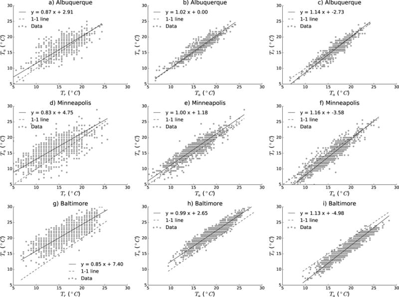
Left column: daily-minimum T_r versus T_u for data from JJA 2000-2015 for a) Albuquerque, d) Minneapolis, and g) Baltimore. Middle column: daily-minimum T_a versus T_u for b) Albuquerque, e) Minneapolis, and h) Baltimore. Right column: daily-minimum T_a versus T_r for c) Albuquerque, f) Minneapolis, and i) Baltimore. The solid line shows the total least squares fit to the data with slope m_daily and dashed line shows the 1-1 line.

We now expand this analysis to 54 cities across the US. The statistical distributions of m_daily are shown in Fig. 2a for all cities. In most cities (38/54), m_daily < 1, meaning that the urban increase is less then the rural increase during warmer conditions. Nationwide, the average response is ${\overline{m}}_{\mathit{daily}}=0.88$. That is, T_u increases on average by only about 0.9° C for every degree increase in daily T_r. The full range of the distribution is 0.11 ≤ m_daily ≤ 1.44 which is statistically different from 1 (p = 0.002). For 16 cities, m_daily > 1, meaning that the UHI increases under warmer conditions. These cities are distributed equally across climate zones (Fig. S2), so their differing behavior is not due to them being in different climate zones. For 10 of the 16 cities where m_daily > 1, the urban weather station is located farther than 10 kilometers from the city center or located in an area with less-developed land cover types (low to no intensity of development). Removing these cities yields ${\overline{m}}_{\mathit{daily}}=0.83$, demonstrating that microclimate effects impact how ΔT changes with heat and explains why cities with increasing UHIs in warmer conditions differ.

Figure 2.

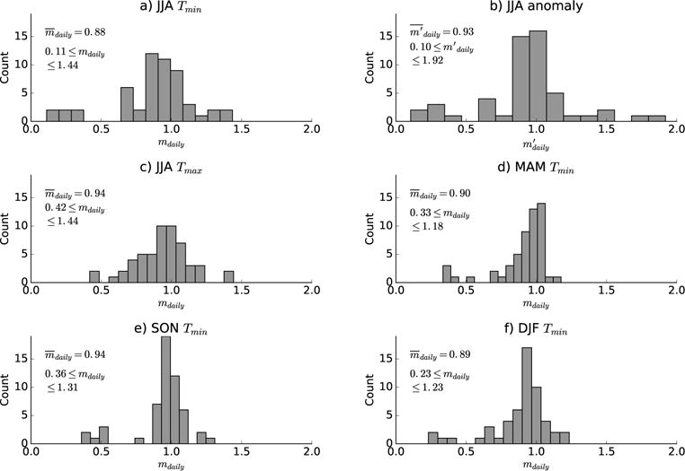
Histograms of m_daily, slope of T_u versus T_r relationship for (a) June, July, August (JJA) daily minimum temperatures, (b) JJA anomaly daily minimum temperatures, (c) JJA daily maximum temperatures, (d) December, January, February (DJF) daily minimum temperatures, (e) March, April, May (MAM) daily-minimum temperatures, and (f) September, October, November (SON) daily-minimum temperatures. The distribution mean ${\overline{m}}_{\mathit{daily}}$ and range are listed in each plot.

The above result that ΔT decreases overall during warmer conditions is robust. Repeating this analysis with daily anomalies calculated with respect to each year’s JJA mean yields a mean sensitivity similar to the raw temperature values ${\overline{m}}_{\mathit{daily}}^{\prime }=0.93(0.1\le m_{\mathit{daily}}^{\prime }\le 1.92)$, see Fig. 2b. This confirms that the decrease of ΔT during warmer conditions is due to day-to-day variability rather than interannual trends. Additionally, a similar relationship between T_r and T_u is also found for daytime (maximum daily) temperatures (Fig. 2c), for other seasons (Fig. 2d-f), and when a longer period is used (1985-2015, Fig. S3). Similarly, varying the weather station selection does not affect the overall result: we find ${\overline{m}}_{\mathit{daily}}=0.84$ when varying urban stations and ${\overline{m}}_{\mathit{daily}}=0.95$ when varying rural stations (Fig. S4, S5). In each case, the mean change is close to 0.9 for day, night, and for all seasons.

It is possible the T_r-T_u relationship may differ during periods of extreme heat, so we next examine how the UHI intensity ΔT evolves during an extreme heat event. We first consider Baltimore, as the change in the UHI during a heatwave in Baltimore has been examined by Li & Bou-Zeid (2013), Li et al. (2014) and Li et al. (2015). Figure 3a, b shows the temporal variation of T_a and ΔT for the 15 hottest nights (heat event night zero) in Baltimore during 2000-2015 (colored lines). T_a rises until heat event night zero and decreases afterwards (Fig. 3a). In contrast, ΔT decreases before night zero and increases after (Fig. 3b). Thus during the four nights before and after these heat events there is a decrease in ΔT. Averaging the 15 events to form a composite event for both T_a and ΔT (Fig. 3a, b, black curves) shows that the average increase in T_a for heat extremes in Baltimore is 5°C with a corresponding decrease of ΔT by 0.1° C.

Figure 3.

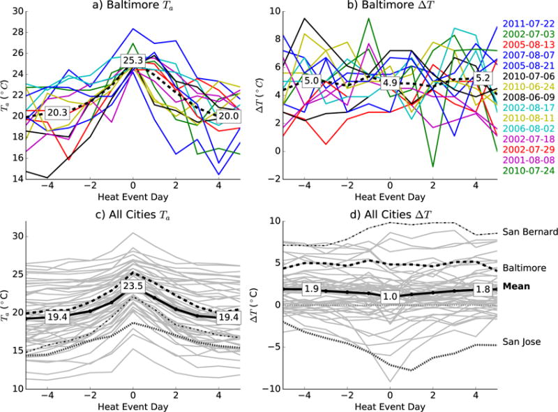
Heat events: a) temporal evolution of T_a for the 15 hottest nights for Baltimore (colors) and their mean (dashed black line), b) temporal evolution of ΔT for those events, c) temporal evolution of T_a averaged across the ten hottest events for each city and the sample mean (heavy black line), and (d) as in (c) but for ΔT.

This result differs from the conclusions of Li & Bou-Zeid (2013), who also examined heat extremes in Baltimore. They considered a single event (5-14 June 2008), during which ΔT increases during the event. This event is included in our analysis in Fig. 3a,b and we find that its behavior is not characteristic as most of the events we find exhibit a decreasing ΔT. Thus, our conclusions differ from Li & Bou-Zeid (2013) because their event is atypical.

Composite heat events from each city are shown in Fig. 3c and d. In 19 cities, ΔT decreases by more than one degree during the heat event (between four days prior and the heat event night zero), in 29 cities, ΔT changes by less than 1°C, and in six cities, ΔT increases by more than 1°C. The distribution of the average change of ΔT during extreme heat, ΔT_hw, is shown in Fig. S6 and the average across all cities is ${\overline{\mathrm{\Delta }T}}_{hw}=-0.9$. This average decrease in ΔT is sufficient to reduce ΔT to below zero on heat event day zero in 18/54 cities, meaning that one third of the examined cities are slightly cooler than surrounding rural areas during the hottest nights.

Cities with UHIs that decrease the most during heat events tend to have larger m_daily (the correlation between m_daily and ΔT_hw is r = 0.7) and 4 of the 6 cities which have an increasing UHI on heat event day zero are also cities for which m_daily > 1. This shows consistency in our results and suggests the same mechanism drives changes in ΔT on daily timescales as well as during periods of extreme heat, and also that the microclimate of urban stations can affect both metrics.

How UHIs respond to heatwaves will depend on the method used for selecting heat events. We repeat the analysis in Fig. 3 by selecting heat events using the hottest urban nights (Fig. S7) and the hottest rural nights (Fig. S8) because when it is hot in one location, it may be less likely to be hot in the second location. As expected, the decrease of ΔT is strongest when selecting using the hottest rural nights. Similarly, an increase of ΔT is observed when selecting the hottest urban nights. However, this increase of ΔT conditioned on hot urban nights is less than the decrease of ΔT conditioned on hot rural nights. Additionally, when selecting events using the first principal component of temperature (Fig. S9), we also see a decrease of ΔT during heat events. We conclude that the decrease of ΔT during heat events is supported by a variety of heat event selection methods.

Given the above robust relationship between ΔT and T_a, an obvious question is what is the cause. It has been suggested that local feedbacks in wind (Haeger-Eugensson & Holmer 1999) and moisture (Li & Bou-Zeid 2013) may modulate the intensity of urban heating. Alternatively, synoptic weather systems could modify the intensity of the heat island by changing humidity, cloudiness, and outgoing longwave radiation. Dry conditions allow rural areas to radiatively cool faster than urban areas, so increasing humidity results in a larger T_r and decreased ΔT. To investigate this, we compute the average ΔT on moist nights, $\mathrm{\Delta }{T}_{\mathit{moist}}={\overline{T}}_u(\mathit{moist})-{\overline{T}}_r(\mathit{moist})$, and compare this with the average ΔT on dry nights, $\mathrm{\Delta }{T}_{\mathit{dry}}={\overline{T}}_u(\mathit{dry})-{\overline{T}}_r(\mathit{dry})$. The distribution of ΔT_moist and ΔT_dry from each city is shown in Fig. 4a. We see that when the surrounding air mass is dry, ΔT tends to be larger: nationwide, ${\overline{\mathrm{\Delta }T}}_{\mathit{dry}}-{\overline{\mathrm{\Delta }T}}_{\mathit{moist}}=0.43°\mathrm{C}$. While small, this difference is statistically significant in most cities (29/46 or 63%). Thus, as has been found in Sheridan, Kalkstein & Scott (2000) and Hardin, Liu, Cao & Vanos (2017), we find weather type as defined in Sheridan (2002) to be an important factor in regulating ΔT.

Figure 4.

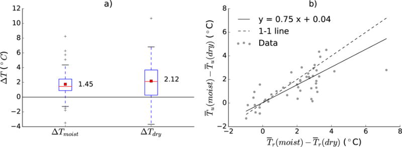
Influence of synoptic weather type: a) nationwide distribution of all city’s mean temperatures for urban and rural stations during moist or dry weather types and b) sensitivity of temperature to synoptic weather conditions for rural (x-axis) versus urban areas (y-axis); the total least squares line is shown in solid black and the 1-1 line is dashed. In a), boxes indicate the middle two quartiles (Q2 and Q3), the red box indicates the mean, the red lines indicate the median, and whiskers represent the wide interquartile range (1.5*(Q3-Q2)). Crosses indicate data points beyond this range, that is, statistical outliers.

As shown in Fig. 1, the daily response to heat occurs primarily in rural rather than urban areas. To assess the sensitivity of urban and rural areas to weather type, we compare the moist-dry temperature difference in each city, ${\overline{T}}_u(\mathit{moist})-{\overline{T}}_u(\mathit{dry})$, against that in each rural area, ${\overline{T}}_r(\mathit{moist})-{\overline{T}}_r(\mathit{dry})$, in Fig. 4b. In most regions there is a tendency for humid nights to be hotter than dry nights; this difference is significant in most cities (39/46 or 85%). That is, T_moist > T_dry for both urban and rural environments. However, see that the values do not follow a one-to-one relationship. Rather, rural areas change substantially by weather type, whereas urban areas do not. During moist synoptic conditions there are higher rural temperatures rather than elevated urban temperatures, which leads to a lower ΔT during moist weather patterns. As these humid weather patterns also tend to be the hottest, the role of synoptic conditions is critical to our result; individual hot events that evolve under less typical hot and dry conditions, or that are influenced by specific mesoscale circulations, may differ in characteristics.

Above, we have shown that ΔT decreases in response to daily temperature increases. This raises the possibility that changes over longer time scales in response to warmer conditions are possible. To test this, we compute the 15-year linear trend in JJA for T_r, called ${\beta }_{T_r}$, for T_u, ${\beta }_{T_u}$, and for T_a, ${\beta }_{T_a}$. We find that most urban and rural areas experience nighttime warming (46/54 or 85%). For each city the urban and rural trends are not similar (r = 0.3) and there is no significant difference between urban and rural trends as calculated by a Student’s t-test (p = 0.63), in agreement with Peterson (2003). Nevertheless, we find that while urban temperatures warm at the same rate as average temperatures, rural temperatures do not (Fig. 5a,b). While 15 years is a limited time period, this result suggests that not only are urban areas not warming faster than rural areas, rural areas may in fact warm faster, though this effect is not significant over the time period measured.

Figure 5.

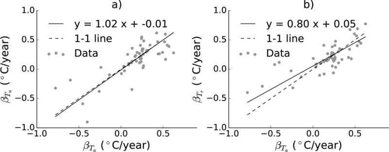
15-year linear trends for each city: a) ${\beta }_{T_r}$ plotted versus ${\beta }_{T_a}$ and b) ${\beta }_{T_u}$ plotted versus ${\beta }_{T_a}$. The total least squares line is shown in solid black and the 1-1 line is dashed.

Above we have shown that differences between T_u and T_r tend to diminish on a variety of time scales, which raises the question of how T_u and T_r varies between cities. To investigate this, we compare the 2000-2015 JJA-mean rural temperature ${\overline{T}}_r$ with the JJA-mean urban temperaure ${\overline{T}}_u$ (Fig. 6a). We see that ${\overline{T}}_u$ tends to be more similar to ${\overline{T}}_r$ for cities with larger ${\overline{T}}_r$, with a slope (sensitivity) of 0.85. That is, the UHI is generally smaller for warmer climates, with T_u increasing on average by only 0.85°C when comparing to a climate zone 1°C warmer. Furthermore, while urban temperatures increase at the same rate as average temperature, rural temperature increase at a faster rate (Fig. 6b,c). That is, when we compare one city to a warmer city, we find the increase in urban temperatures is similar to the increase in average temperature. The increase in rural temperatures, however, is more than the increase in average temperatures, resulting in a decreased ΔT for warmer cities. Thus, the tendency for a weaker ΔT under warmer conditions occurs not only on daily time-scales in individual cities but also between cities.

Figure 6.

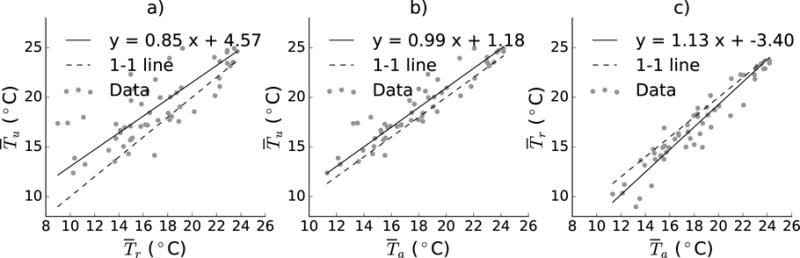
15 year mean temperature for each city: a) ${\overline{T}}_r$ versus ${\overline{T}}_u$, b) ${\overline{T}}_r$ versus ${\overline{T}}_a$, and ${\overline{T}}_u$ versus ${\overline{T}}_a$. The total least squares line is shown in solid black and the 1-1 line is dashed.

Concluding remarks

We have compared daily maximum and minimum urban and rural temperatures using station observations from 54 US cities for 2000-2015, and shown that in most cities, the intensity of the UHI, ΔT, diminishes with warmer temperatures. This holds over temporal scales—daily over the entire summer, during extreme heat—as well as across climate zones. For daily variability T_u increases on average by only 0.88 °C for every degree increase in T_r, while the average decrease of T_u during extreme heat is 0.93 °C. On interannual timescales, we find that urban trends have a one-to-one relationship with average temperature trends, meaning the UHI has not increased with climate change, but do note that rural trends decreased slightly with increasing average trends. We relate the decrease in ΔT with larger T_r to large-scale or synoptic weather conditions, and find that the lowest ΔT nights occur during moist conditions. Further, we find that across all time and space scales, our results are driven by changes in rural temperatures rather than urban temperatures, which appear less sensitive to both heat and weather type.

Our results differ from previous studies because we examine more cities, longer time periods, and more heat events. Conclusions of an increasing UHI during warmer temperatures were based on studies of single cities and single events. For example, the previous study of Baltimore (Li & Bou-Zeid 2013) only examined one heat event; we examine this event and others in addition to 15 years of daily data and find that the event in Li & Bou-Zeid (2013) is atypical. We do find some individual cities for which UHI increases with warmer temperatures, however, in most cases, we find this to be related to the land type and thus microclimate of the weather station, similar to Zhou & Shepherd (2010).

The decrease in UHI intensity with warmer conditions has potentially important implications for accounting for urbanization in long term climate records, where it is often assumed that absent significant changes in urban extent, the urban and rural areas warm at the same rate (Hausfather, Menne, Williams, Masters, Broberg & Jones 2013, Stone et al. 2012). Perhaps more importantly, it has implications for changes in the UHI as climate continues to warm as well as for economic projections of climate change impacts for cities (Estrada et al. 2017). That warming areas did not experience any increase in urban heating indicates that the nighttime urban heat island has not been exacerbated by climate change. Absent consideration of changes in synoptic weather patterns, urbanization, or urban extent, our results suggest that the urban heat island as defined by available weather stations may remain constant or possibly decline as background climate warms. Indeed, there is already a tendency for T_r > T_u on the hottest nights for many cities (e.g., Fig. 3d).

We emphasize that our results do not mean that global warming will not affect cities, but rather that surrounding rural areas may warm faster than urban areas absent changes in urbanization and urban extent. Furthermore, the moist weather types which we associate with low UHI nights, in particular the moist tropical weather type, are associated with elevated risks for mortality and morbidity (Sheridan & Kalkstein 2004), meaning that lower UHIs will not necessarily translate into lower health risks. This is important for heat mitigation efforts, economic projections, and climate resiliency plans to take into account, as our results suggest that rural and suburban heat mitigation efforts may be more important than previously thought. Health analyses are concerned with physiologically relevant temperature thresholds, and our results indicate that assumptions of a constant or increasing urban heat may mischaracterize those risks.

References

- Aerts JC, Botzen WW, Emanuel K, Lin N, de Moel H, Michel-Kerjan EO. Evaluating flood resilience strategies for coastal megacities. Science. 2014;344(6183):473–475. doi: 10.1126/science.1248222. [DOI] [PubMed] [Google Scholar]
- Allen M, Stott P. Estimating signal amplitudes in optimal fingerprinting, part I: Theory. Climate Dynamics. 2003;21(5–6):477–491. [Google Scholar]
- Arnfield AJ. Two decades of urban climate research: a review of turbulence, exchanges of energy and water, and the urban heat island. International Journal of Climatology. 2003;23(1):1–26. [Google Scholar]
- Coffee JE, Parzen J, Wagstaff M, Lewis RS. Preparing for a changing climate: The Chicago climate action plan’s adaptation strategy 2010 [Google Scholar]
- DMSP, D. M. S. P. Operational linescan system (DMSP/OLS) 2013 [Google Scholar]
- Estrada F, Tol RS, Botzen WJ. Global economic impacts of climate variability and change during the 20th century. PloS one. 2017;12(2):e0172201. doi: 10.1371/journal.pone.0172201. [DOI] [PMC free article] [PubMed] [Google Scholar]
- Gabriel KM, Endlicher WR. Urban and rural mortality rates during heat waves in Berlin and Brandenburg, Germany. Environmental pollution. 2011;159(8):2044–2050. doi: 10.1016/j.envpol.2011.01.016. [DOI] [PubMed] [Google Scholar]
- Georgescu M, Morefield PE, Bierwagen BG, Weaver CP. Urban adaptation can roll back warming of emerging megapolitan regions. Proceedings of the National Academy of Sciences. 2014;111(8):2909–2914. doi: 10.1073/pnas.1322280111. [DOI] [PMC free article] [PubMed] [Google Scholar]
- Gorelick N, Hancher M, Dixon M, Ilyushchenko S, Thau D, Moore R. Google earth engine: Planetary-scale geospatial analysis for everyone. Remote Sensing of Environment. 2017 doi: 10.1016/j.rse.2017.06.031. URL: [DOI]
- Haeger-Eugensson M, Holmer B. Advection caused by the urban heat island circulation as a regulating factor on the nocturnal urban heat island. International Journal of Climatology. 1999;19(9):975–988. [Google Scholar]
- Hardin A, Liu Y, Cao G, Vanos J. Urban heat island intensity and spatial variability by synoptic weather type in the northeast us. Urban Climate 2017 [Google Scholar]
- Hausfather Z, Menne MJ, Williams CN, Masters T, Broberg R, Jones D. Quantifying the effect of urbanization on US Historical Climatology Network temperature records. Journal of Geophysical Research: Atmospheres. 2013;118(2):481–494. [Google Scholar]
- Homer C, Dewitz J, Yang L, Jin S, Danielson P, Xian G, Coulston J, Herold N, Wickham J, Megown K. Completion of the 2011 national land cover database for the conterminous united states–representing a decade of land cover change information. Photogrammetric Engineering & Remote Sensing. 2015;81(5):345–354. [Google Scholar]
- Kalnay E, Cai M. Impact of urbanization and land-use change on climate. Nature. 2003;423(6939):528–531. doi: 10.1038/nature01675. [DOI] [PubMed] [Google Scholar]
- Lawrimore JH, Menne MJ, Gleason BE, Williams CN, Wuertz DB, Vose RS, Rennie J. An overview of the global historical climatology network monthly mean temperature data set, version 3. Journal of Geophysical Research: Atmospheres. 2011;116(D19) [Google Scholar]
- Li D, Bou-Zeid E. Synergistic interactions between urban heat islands and heat waves: the impact in cities is larger than the sum of its parts. Journal of Applied Meteorology and Climatology. 2013;52(9):2051–2064. [Google Scholar]
- Li D, Bou-Zeid E, Oppenheimer M. The effectiveness of cool and green roofs as urban heat island mitigation strategies. Environmental Research Letters. 2014;9(5):055002. [Google Scholar]
- Li D, Sun T, Liu M, Yang L, Wang L, Gao Z. Contrasting responses of urban and rural surface energy budgets to heat waves explain synergies between urban heat islands and heat waves. Environmental Research Letters. 2015;10(5):054009. [Google Scholar]
- Luber G, McGeehin M. Climate change and extreme heat events. American Journal of Preventive Medicine. 2008;35(5):429–435. doi: 10.1016/j.amepre.2008.08.021. [DOI] [PubMed] [Google Scholar]
- Menne MJ, Williams CN, Jr, Vose RS. The US Historical Climatology Network monthly temperature data, version 2. Bulletin of the American Meteorological Society. 2009;90(7):993–1007. [Google Scholar]
- Peng S, Piao S, Ciais P, Friedlingstein P, Ottle C, Bréon FM, Nan H, Zhou L, Myneni RB. Surface urban heat island across 419 global big cities. Environmental Science & Technology. 2011;46(2):696–703. doi: 10.1021/es2030438. [DOI] [PubMed] [Google Scholar]
- Peterson TC. Assessment of urban versus rural in situ surface temperatures in the contiguous United States: No difference found. Journal of Climate. 2003;16(18):2941–2959. [Google Scholar]
- Pitkänen MR, Mikkonen S, Lehtinen KE, Lipponen A, Arola A. Artificial bias typically neglected in comparisons of uncertain atmospheric data. Geophysical Research Letters. 2016;43(18) [Google Scholar]
- Ramamurthy P, Li D, Bou-Zeid E. High-resolution simulation of heatwave events in New York City. Theoretical and Applied Climatology. 2017;128(1–2):89–102. [Google Scholar]
- Schatz J, Kucharik CJ. Urban climate effects on extreme temperatures in Madison, Wisconsin, USA. Environmental Research Letters. 2015;10(9):094024. [Google Scholar]
- Scott AA, Zaitchik B, Waugh D, O’Meara K. Intra-urban temperature variability in Baltimore. Journal of Applied Meteorology and Climatology. 2016 (2016) [Google Scholar]
- Sharma A, Conry P, Fernando H, Hamlet AF, Hellmann J, Chen F. Green and cool roofs to mitigate urban heat island effects in the Chicago metropolitan area: evaluation with a regional climate model metropolitan area: evaluation with a regional climate model. Environ Res Lett. 2016;11(6):64004. [Google Scholar]
- Sheridan SC. The redevelopment of a weather-type classification scheme for North America. International Journal of Climatology. 2002;22(1):51–68. [Google Scholar]
- Sheridan SC, Kalkstein LS. Progress in heat watch–warning system technology. Bulletin of the American Meteorological Society. 2004;85(12):1931–1941. [Google Scholar]
- Sheridan SC, Kalkstein LS, Scott JM. An evaluation of the variability of air mass character between urban and rural areas. Biometeorology and Urban Climatology at the Turn of the Millennium. 2000:487–490. [Google Scholar]
- Stone B, Vargo J, Habeeb D. Managing climate change in cities: will climate action plans work? Landscape and Urban Planning. 2012;107(3):263–271. [Google Scholar]
- WMO. Atlas of mortality and economic losses from weather, climate, and water extremes (1970–2012) Geneva, Switzerland: World Meteorological Organization; 2014. URL: https://search.library.wisc.edu/catalog/9910206226102121. [Google Scholar]
- Zhao L, Lee X, Smith RB, Oleson K. Strong contributions of local background climate to urban heat islands. Nature. 2014;511(7508):216–219. doi: 10.1038/nature13462. [DOI] [PubMed] [Google Scholar]
- Zhou Y, Shepherd JM. Atlanta’s urban heat island under extreme heat conditions and potential mitigation strategies. Natural Hazards. 2010;52(3):639–668. [Google Scholar]
Associated Data
This section collects any data citations, data availability statements, or supplementary materials included in this article.