AnatomiCuts: Hierarchical Clustering of Tractography Streamlines Based on Anatomical Similarity

Abstract

Diffusion MRI tractography produces massive sets of streamlines that contain a wealth of information on brain connections. The size of these datasets creates a need for automated clustering methods to group the streamlines into meaningful bundles. Conventional clustering techniques group streamlines based on their spatial coordinates. Neuroanatomists, however, define white-matter bundles based on the anatomical structures that they go through or next to, rather than their spatial coordinates. Thus we propose a similarity measure for clustering streamlines based on their position relative to cortical and subcortical brain regions. We incorporate this measure into a hierarchical clustering algorithm and compare it to a measure that relies on Euclidean distance, using data from the Human Connectome Project. We show that the anatomical similarity measure leads to a 20% improvement in the overlap of clusters with manually labeled tracts. Importantly, this is achieved without introducing any prior information from a tract atlas into the clustering algorithm, therefore without imposing the existence of any named tracts.

1. Introduction

Diffusion MRI (dMRI) allows us to estimate the preferential direction of water molecule diffusion at each voxel in the white matter (WM) (Le Bihan et al., 1986). Tractography algorithms follow these directions to reconstruct continuous paths of diffusion (Mori et al., 1999; Basser et al., 2000). The most common approach to segmenting the WM from dMRI data is to use every voxel in the brain as a seed for tractography and to group the resulting streamlines into bundles. Recent advances in dMRI acquisition hardware and software (Wright & Wald, 1997; Setsompop et al., 2013) have increased both spatial and angular resolution, yielding large tractography datasets that are difficult to parse manually. This creates a need for computational methods that can group streamlines into anatomically meaningful bundles automatically.

Several unsupervised clustering algorithms have been proposed to assign tractography streamlines into bundles. Each method is characterized by (i) the measure that it uses to quantify the similarity between two streamlines and (ii) the algorithm that it follows to group streamlines based on their similarity.

Typical similarity measures for unsupervised clustering of streamlines are functions of the streamline coordinates in Euclidean space. These measures express either the distance between streamlines (Ding et al., 2003; Gerig et al., 2004; Moberts et al., 2005; Tsai et al., 2007; Wassermann et al., 2010; Visser et al., 2011; Siless et al., 2013) or the similarity of some shape descriptor computed from spatial coordinates (Gerig et al., 2004; Brun et al., 2004; Ros et al., 2013; Zhang et al., 2014). A subset of these methods use the distance metrics to project the streamlines onto an eigenspace and perform the clustering in that space (Tsai et al., 2007; O’Donnell & Westin, 2007).

However, bundling streamlines based on their proximity or their shape is not consistent with the approach followed by neuroanatomists. In neuroanatomy, WM bundles are defined based on the brain structures that they go through or next to, rather than their coordinates in a reference space. For example, “The uncinate fasciculus extends between the anterior temporal lobe and the frontal lobe passing though the floor of the insula in an area between the anterior claustrum and the amygdala” (Makris & Pandya, 2008). Here we propose a similarity measure that adopts the neuroanatomist’s approach of comparing streamlines based on their anatomical neighborhood.

Previous attempts to incorporate anatomical information in unsupervised streamline clustering used the structures that the streamlines terminate in, either in the similarity measure itself (Tunc et al., 2014), in a post-hoc manner (Wassermann et al., 2010), or for initialization (Guevara et al., 2011). Alternatively, supervised clustering approaches introduced prior information on WM anatomy from an atlas of predefined bundles, labeled by an expert (O’Donnell & Westin, 2007; Maddah et al., 2008; Ziyan et al., 2009; Guevara et al., 2012; Wang et al., 2013; Ros et al., 2013; Jin et al., 2014). Another class of supervised methods used deterministic rules on the position of streamlines with respect to anatomically defined regions, thus going directly from the whole-brain tractography data to a set of pre-determined WM bundles (Xia et al., 2005; Li et al., 2010; Wassermann et al., 2016). In Xia et al. (2005) and Li et al. (2010) clustering based on Euclidean distance was performed as a subsequent step, to refine these bundles, but the anatomical regions were only used in the form of deterministic rules before that clustering step.

In this work we propose an anatomical similarity measure for unsupervised streamline clustering that uses not only the anatomical regions that the streamlines terminate in, but all regions that form the anatomical neighborhood of a streamline, everywhere along its trajectory. We have previously used a similar description of anatomical neighborhoods to incorporate prior information from a set of training subjects into the tractography step itself (Yendiki et al., 2011). However, that was a supervised approach, limited to a set of predefined bundles from an atlas. Here we are interested in exploratory studies that do not rely on training data. Therefore, we do not impose the existence of any named pathways based on a WM atlas; instead, we cluster whole-brain tractography streamlines based on their position with respect to a set of cortical and subcortical structures.

The algorithms that have been used for unsupervised streamline clustering are either partitioning or hierarchical. Partitioning approaches include K-means (Tsai et al., 2007; O’Donnell & Westin, 2007; Siless et al., 2013), affinity propagation (Zhang et al., 2014), maximum likelihood (Maddah et al., 2008), and maximum a posteriori (Wang et al., 2011; Tunc et al., 2014). Hierarchical algorithms that have been applied to unsupervised streamline clustering are either agglomerative or divisive. Agglomerative algorithms follow a bottom-up approach, first assigning each streamline to its own cluster and then merging clusters iteratively (Ding et al., 2003; Gerig et al., 2004; Wassermann et al., 2010; Visser et al., 2011; Guevara et al., 2012; Ros et al., 2013). Divisive algorithms follow a top-down approach, first assigning all streamlines to a single cluster and then splitting clusters iteratively (Brun et al., 2004; Ziyan et al., 2009; Wu et al., 2012). Hierarchical methods organize streamlines into a tree structure, where larger clusters are composed of smaller clusters. This is particularly suitable for describing WM organization, as anatomical tracing studies have revealed that the large WM pathways are subdivided into multiple smaller bundles that share a large part of their trajectory but originate or terminate in different brain regions (Lehman et al., 2011). Hence we follow the hierarchical approach here.

Our proposed method, AnatomiCuts, incorporates an anatomical similarity measure into normalized cuts, an algorithm that has been used previously for streamline clustering with conventional similarity measures (Brun et al., 2004; O’Donnell et al., 2006; Ziyan et al., 2009). We follow an implementation of normalized cuts where a hierarchy of clusters is generated by recursive bipartitions of the full data set (Shi & Malik, 2000; Brun et al., 2004). The present work expands on a prior conference publication (Siless et al., 2016), by adding much more extensive experimental results on the performance of the proposed method and the effects of various tuning parameters that are involved in its implementation.

Specifically, we compare the performance of our anatomical similarity measure to one based on Euclidean distance between streamlines, using data from the MGH-USC Human Connectome Project. We show that clustering streamlines based on their anatomical neighborhood rather than their spatial coordinates leads to a 20% improvement in the agreement of the clusters with WM bundles labeled manually by a human rater. Importantly, we achieve this improvement without using prior information from clusters labeled manually in training subjects; we only use a subject’s own anatomical segmentation. Our approach is unsupervised, allowing exploratory studies of whole-brain tractography data, without being constrained to a predetermined set of bundles.

2. Methods

2.1. Similarity measures

Let f_i be a tractography streamline, defined as a sequence of N points, f_i = [x_i1,′,x_iN], where ${\mathbf{x}}_{\mathit{ik}}\in {\mathbb{R}}^3$, k = 1,′, N. A tractography dataset is a set of M streamlines, F = {f₁,′, f_M}.

In the following, we assume that all streamlines have the same number of points N. Although the similarity measures can be adapted to streamlines with variable numbers of points, the approach of downsampling streamlines to an equal number of points has been used previously by others to make computation tractable (O’Donnell & Westin, 2007; Visser et al., 2011; Garyfallidis et al., 2012; Guevara et al., 2012; Wu et al., 2012; Siless et al., 2013).

2.1.1. Euclidean similarity

We define a similarity measure based on the mean Euclidean distance between pairs of points on two streamlines f_i and f_j, as previously used in the literature (Visser et al., 2011; Garyfallidis et al., 2012; Guevara et al., 2012; Wu et al., 2012; Siless et al., 2013):

$${\omega }_{\mathrm{E}}({\mathbf{f}}_i,{\mathbf{f}}_j)\triangleq {\left(1+\frac{1}{N}\sum _{k=1}^N{\Vert {\mathbf{x}}_{\mathit{ik}}-{\mathbf{x}}_{\mathit{jk}}\Vert }^2\right)}^{-1}.$$

Since the ordering of points is not consistent across streamlines, it is possible for the first point of f_i to be closer to the last point of f_j and vice versa. We account for this by also evaluating the similarity between f_i and the reversed f_j. This leads to the following definition for the similarity measure:

$${\omega }_{\mathrm{E}}({\mathbf{f}}_i,{\mathbf{f}}_j)\triangleq \text{max}\{{\omega }_{\mathrm{E}}({\mathbf{f}}_i,{\mathbf{f}}_j),{\omega }_{\mathrm{E}}({\mathbf{f}}_i,{\mathbf{f}}_j^{\text{rev}})\},$$ (1)

where ${\text{f}}_j^{rev}$ = [x_jN,′, x_j1].

Another option for converting a Euclidean distance into a similarity measure is by means of a Gaussian kernel. However that formulation involves the choice of a kernel width, and the optimal width can vary greatly depending on the input (Brun et al., 2004; O’Donnell & Westin, 2007). Here we opt for a similarity measure that does not involve free parameters (Sammut & Webb, 2017).

2.1.2. Anatomical similarity

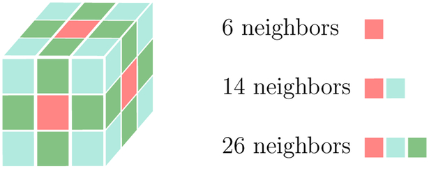
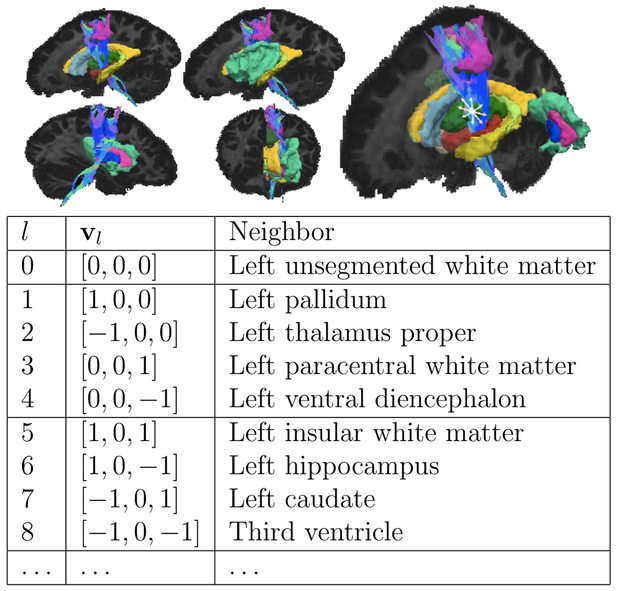
We introduce a new similarity measure that uses anatomical information in the form of a cortical and subcortical segmentation, S(x), $\mathbf{x}\in {\mathbb{R}}^3$. This is done by finding the segmentation labels that each streamline goes through or next to, at each point along its trajectory. Specifically, each point x on a streamline is associated with a set of segmentation labels, S(x + d_l(x)v_l), l = 1,′, P, where d_l(x) is the minimum d > 0 such that S(x+d_vl) ≠ S(x). That is, for each point x, we find the nearest neighboring segmentation labels in a set of directions v_l, l = 1,′, P. A neighborhood of P = 26 elements includes neighboring labels in the directions v_l = [e₁, e₂, e₃], where e_1,2,3 ∈ {−1, 0, 1}. We also define v₀ = [0, 0, 0] to represent the segmentation label that the streamline passes through. Fig. 1 shows an illustration of this neighborhood. Fig. 2 shows an example of a point in the WM and some of its neighboring segmentation labels in different directions.

Figure 1:

Directions in which nearest neighboring segmentation labels are found, for a streamline point that lies in the center of the cube. Red directions belong to the 6, 14 and 26-element neighborhoods. Blue directions belong to the 14 and 26-element neighborhoods. Green directions belong only to the 26-element neighborhood.

Figure 2:

Example of the anatomical neighborhood of a point in the corticospinal tract. Neighboring FreeSurfer segmentation labels in the L-R and I-S directions are shown in the table.

For each direction l = 0, ′ P, we compute a label histogram ${\mathbf{H}}_{il}\in {\mathbb{R}}^K$, where K is the total number of labels in the anatomical segmentation. This histogram represents the frequency with which different segmentation labels are the l-th neighbor across all points on the i-th streamline. We introduce a similarity measure between two streamlines f_i and f_j that expresses the joint probability of their anatomical neighborhoods. We define this anatomical similarity measure as:

$$w_{\mathrm{A}}({\mathbf{f}}_i,{\mathbf{f}}_j)\triangleq \mid L_i\cap L_j\mid \sum _{l=0}^P\langle {\mathbf{H}}_{\mathit{il}},{\mathbf{H}}_{\mathit{jl}}\rangle ,$$ (2)

where ⟨·, ·⟩ is the inner product, and L_i, L_j are the sets of all labels found to be neighbors of streamlines f_i, f_j. The normalization factor ∣L_i∩L_j∣, which is the number of common neighbors between the two streamlines, penalizes trivial streamlines with too few neighbors.

2.2. Normalized cuts

We approach clustering as a graph partitioning problem, where the nodes of the graph are the elements to be clustered and the weights of the edges between nodes are the similarities between elements. These weights are used to form a similarity matrix, and clusters are defined based on the eigenvectors of this matrix. Given a connected graph G, the normalized cuts algorithm searches for a graph cut that divides G into sets A and B (A ∩ B = ∅), by minimizing similarity between A and B and maximizing similarity within A and B (Shi & Malik, 2000). Clusters are split recursively, generating a top-down hierarchical structure.

When clustering tractography data, each streamline represents a node on a graph G, and the weight of each edge is the similarity between the nodes it connects. In this case graph G is a clique, and thus each streamline is connected to every other streamline. For the purpose of finding the optimal cut of the graph into A and B, we need to quantify the similarity between A and B. This is done by summing the weights of the edges that connect them: s(A, B) = Σ_u∈A,v∈Bw(u,v), where w(·, ·) is a similarity function between two streamlines. To avoid trivial solutions where A or B is a single isolated node, s is normalized by an association measure a(A) = Σ_u∈A,t∈Gw(u,t). Thus the minimum cut is defined based on the following cost function:

$$\underset{A,B}{\text{min}}{s}_{\text{norm}}(A,B)s_{\text{norm}}(A,B)=\frac{s(A,B)}{a(A)}+\frac{s(A,B)}{a(B)}.$$ (3)

We can formulate this equation with matrix notation where W is the similarity matrix with W_ij = w(i, j), D is a diagonal matrix with D_ii = Σ_j w(i, j) and x the partitioning vector, where x_i = 1 if the i-th element belongs to A and x_i = −1 is the i-th element belongs to B. The association measure will be encoded in $k=\frac{{\sum }_{x_i>0}{d}_i}{\sum d_i}$

$$s_{\text{norm}}(A,B)=\frac{{(1+\mathbf{x})}^T(\mathbf{D}-\mathbf{W})(1+\mathbf{x})}{k{1}^{T}D1}+\frac{{(1+\mathbf{x})}^T(\mathbf{D}-\mathbf{W})(1+\mathbf{x})}{(1-k)1^{T}D1}.$$

The problem is embedded in the real-valued domain and can be efficiently solved by the following equation (Shi & Malik, 2000):

$${\mathbf{D}}^{\frac{1}{2}}(\mathbf{D}-\mathbf{W}){\mathbf{D}}^{\frac{1}{2}}\mathbf{z}=\lambda \mathbf{z},$$ (4)

where z = Dy, and D – W is a Laplacian matrix.

The second eigenvector of the Laplacian matrix is a solution to the above equation. The optimal cut is approximated by assigning the i-th node to A if y_i > 0, where $y_i\in \mathbb{R}$ is the i-th element of y, and to B otherwise (Golub & Van Loan, 1996). The algorithm is run iteratively by cutting the largest remaining cluster, until a desired number of clusters is reached or a threshold for minimum cluster size or dispersion is met.

2.3. Prototype streamlines

Building an affinity matrix requires computing the similarity between every pair of streamlines, which is extremely time- and memory-intensive for the large, high-resolution data sets that are increasingly common. In previous work, the size of the affinity matrix was reduced by processing left, right, and inter-hemisphere streamlines separately (Guevara et al., 2012); by using a random subset of streamlines to guide the clustering of the full set (O’Donnell & Westin, 2007; Siless et al., 2013; Ros et al., 2013; Zhang et al., 2014); or by generating clustering solutions from multiple subsets of streamlines and merging them (Visser et al., 2011).

The approach of using a subset of the streamlines to compute the affinity matrix has been advocated as a way to reduce sensitivity to outliers in hierarchical clustering (Guha et al., 2001). When clustering tractography data, each bundle contains hundreds to thousands of similar streamlines, resulting in redundancy. Therefore it is reasonable to expect a subset of streamlines to be sufficient for capturing the general shape of the clusters. In the divisive algorithm that we use in this work, we evaluate the similarity matrix to make a binary cut. In early stages of the algorithm, where computational demands are highest because of the large number of streamlines to be divided, these divisions are rather coarse (for example, separating the left hemisphere from the right hemisphere, or the SLF from the arcuate fasciculus). This means that we only need to select enough streamlines to ensure that we have representive examples from these coarse sets.

Here we select a random subset of the streamlines to be clustered at each iteration. We generate the affinity matrix from this subset, which we refer to as prototype streamlines. After finding the minimum cut for the prototype streamlines, we assign each non-prototype streamline to the same cluster as its closest prototype streamline. As part of the experiments described below, we investigate the effect that the number of prototype streamlines has on the performance of our method.

2.4. Data acquisition

For the experimental evaluation of our unsupervised clustering, we use dMRI and structural MRI (sMRI) data from 32 healthy subjects, available publicly through the MGH-USC Human Connectome Project (http://humanconnectomeproject.org). The data was acquired on the MGH Siemens Connectom, a Skyra 3T MRI system with a custom gradient capable of maximum strength 300 mT/m and slew rate 200 T/m/s (Setsompop et al., 2013). The sMRI data was acquired with MEMPRAGE (Mugler & Brookeman, 1990; Van der Kouwe et al., 2008), TR=2530ms, TE=1.15ms, TI=1100ms, 1mm isotropic resolution. The dMRI data was acquired with 2D EPI, TR=8800ms, TE=57ms, 1.5mm isotropic resolution, 512 gradient directions, b_max = 10, 000s/mm². The data were pre-processed as described in Fan et al. (2016).

2.5. Data analysis

We reconstruct orientation distribution functions from the dMRI data using the generalized q-sampling imaging model (Yeh et al., 2010) and perform whole-brain deterministic tractography using DSI Studio (Yeh et al., 2013). We seed every voxel in the segmentation map computed by FreeSurfer. Previously, separate processing strategies have been proposed for longer vs. shorter streamlines (Guevara et al., 2012; Zhang et al., 2014). Here we focus on long-range connections, as short-range connections, such as those representing U-fibers, could be clustered simply based on the anatomical regions that they terminate in. To obtain a large number of long-range connections while keeping computation tractable, we generate a total of 500,000 streamlines per subject and then exclude any streamlines shorter than 55mm, leaving between 100,000 and 150,000 streamlines per subject. We downsample all streamlines to N = 10 equispaced points.

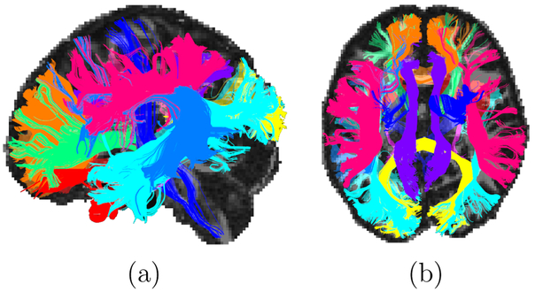
For comparison with our unsupervised clustering, we use a set of major WM bundles labeled manually in each subject by a trained rater, following the protocol described in Wakana et al. (2007). This includes the following bundles: corticospinal tract (CST), inferior longitudinal fasciculus (ILF), uncinate fasciculus (UNC), anterior thalamic radiation (ATR), cingulum - supracallosal bundle (CCG), cingulum - infracallosal (angular) bundle (CAB), superior longitudinal fasciculus - parietal bundle (SLFP), superior longitudinal fasciculus - temporal bundle (SLFT), corpus callosum - forceps major (FMAJ), corpus callosum - forceps minor (FMIN). The intra-hemispheric bundles, i.e., all except FMAJ and FMIN, are labeled on both hemispheres (L and R), leading to a total of 18 manually labeled WM bundles per subject. The rater interacts with the whole-brain tractography data in TrackVis (http://trackvis.org), using the fractional anisotropy map and the color-coded map of the primary eigenvector of the tensor for anatomical guidance. For each of the bundles, at least two inclusion masks are hand-drawn on slices of those maps (as specified in Wakana et al. (2007)) to isolate the streamlines that belong to the bundle. Additional inclusion and exclusion masks are drawn as needed to refine the labeling. Fig. 3 shows the 18 manually labeled WM bundles from an example subject.

Figure 3:

Sagittal (a) and axial (b) view of the 18 manually labeled bundles that we use for comparison to the unsupervised clustering results, shown in a randomly selected subject.

Anatomical segmentations are obtained by processing the sMRI data with the automated cortical parcellation and subcortical segmentation tools in FreeSurfer (Fischl et al., 2002, 2004). As part of this processing, subcortical WM labels are defined by classifying each WM voxel that is within 5mm from the cortex based on its nearest cortical label. This results in a total of K = 261 cortical and subcortical labels. Each subject’s dMRI and sMRI data are aligned with a within-subject, boundary-based, affine registration method, which optimizes the contrast of the b = 0 dMRI volumes across the grey-white boundary surfaces reconstructed from the sMRI data (Greve & Fischl, 2009). The subject’s anatomical segmentation is then mapped from sMRI space to dMRI space by applying the inverse of that transformation.

For each subject, we perform unsupervised clustering with normalized cuts and each of the two similarity measures defined in section 2.1. As the selection of the total number of clusters is arbitrary, we evaluate the effect of this number throughout our experiments. We do this by running the clustering algorithm until a total of 200 clusters are generated, and then pruning the hierarchical clustering tree to keep the first 75, 100, 125, 150 or 200 clusters.

2.6. Evaluation metrics

2.6.1. Comparison with manual labeling

For each subject, we evaluate the extent to which the clusters obtained with each of the two similarity measures resemble bundles labeled by a human rater in the same subject. First, we compute the overlap, as quantified by the Dice coefficient (Dice, 1945; Sørensen, 1948), between each manually labeled bundle and the union of all clusters for which at least 5% of streamlines belong to the manually labeled bundle. The goal of this evaluation is to determine the extent to which streamlines that a human rater would classify into a single anatomical structure become divided among disparate clusters.

Second, we compute the homogeneity and the completeness of each cluster of streamlines with respect to the 18 manually labeled bundles in each subject. These measures are defined in Rosenberg & Hirschberg (2007). Homogeneity is highest when each cluster contains elements from a single manually labeled bundle only and completeness is highest when elements from the same manually labeled bundle are assigned to a single cluster. It is important to evaluate both measures, as it is possible to achieve perfect homogeneity by compromising completeness, i.e., by assigning each streamline to its own cluster.

2.6.2. Anatomical and spatial consistency of clusters

One might expect streamlines that are close to each other in Euclidean space to also have common anatomical neighbors, and vice versa. Hence, we evaluate the extent to which streamlines that are clustered based on the anatomical similarity measure w_A are also similar with respect to the Euclidean similarity measure w_E and vice versa. To this end, we find the centroid of each cluster, defined as the streamline closest to the average of all streamlines in a cluster. We then evaluate w_E and w_A between every element in a cluster and the cluster centroid.

We also compute a distance metric that neither the w_E-optimal nor the w_A-optimal clusters are optimized for. This is the mean of the closest-point distance (Corouge et al., 2004; Moberts et al., 2005; O’Donnell et al., 2006; Guevara et al., 2012) between two streamlines f_i and f_j, defined as:

$${\omega }_{\text{CP}}({\mathbf{f}}_i,{\mathbf{f}}_j)\triangleq \frac{1}{N}\sum _{k=1}^N\underset{l=1}{\overset{N}{\text{min}}}{\Vert {\mathbf{x}}_{\mathit{ik}}-{\mathbf{x}}_{\mathit{jl}}\Vert }^2,$$

where ω_CP(f_i, f_j) and ω_CP(f_j, f_j) are averaged to ensure symmetry:

$${\omega }_{\text{CP}}({\mathbf{f}}_i,{\mathbf{f}}_j)\triangleq \frac{1}{2}({\omega }_{\text{CP}}({\mathbf{f}}_i,{\mathbf{f}}_j)+{\omega }_{\text{CP}}({\mathbf{f}}_j,{\mathbf{f}}_i)).$$ (5)

In our case, f_j is the centroid of the cluster that f_j belongs to.

2.6.3. Robustness to errors in the anatomical segmentation

As our proposed similarity measure relies on an anatomical segmentation, we evaluate the robustness of the clustering to errors in the boundaries of the anatomical segmentation labels. To this end, we perturb the boundaries of the FreeSurfer cortical and subcortical segmentation labels in each subject, and repeat the clustering using the perturbed segmentation. We perform the perturbations by replacing the segmentation label of each voxel with a label selected randomly among the labels of its neighboring voxels. This is done on segmentations that have been mapped into dMRI space, thus the perturbations are in the order of the dMRI voxel size (1.5mm). To establish that this is comparable to the actual accuracy of the FreeSurfer anatomical segmentation, we also show plots of the mean closest point distance between automatically segmented and manually labeled brain structures in 26 subjects from the FreeSurfer atlas. We note that no manual editing has been performed on the FreeSurfer reconstructions that we use in our experiments.

2.6.4. Effect of prototype streamlines

For the evaluations described above, we used 500 randomly selected prototype streamlines to compute the similarity matrices. We assess the impact of this choice by repeating the clustering using 5 different sets of 500 prototype streamlines, and also by varying the number of prototype streamlines between 50 and 3000.

2.6.5. Effect of anatomical neighborhood size

For the evaluations described above, we computed our anatomical similarity measure using the 26-element neighborhood from Fig. 1. We investigate the impact of this neighborhood size by repeating the clustering with the 6-element and 14-element anatomical neighborhoods.

2.6.6. Effect of streamline downsampling

When computing the distance of tractography streamlines in Euclidean space, it is common for clustering algorithms to downsample streamlines to a constant number of points N (O’Donnell & Westin, 2007; Visser et al., 2011; Garyfallidis et al., 2012; Guevara et al., 2012; Wu et al., 2012; Siless et al., 2013). This reduces computation time for Euclidean distances dramatically, as it makes the task of finding corresponding points between two streamlines trivial. Although our anatomical similarity measure does not require all streamlines to have an equal number of points, we did downsample streamlines for the purpose of comparing to the Euclidean distance measure. We evaluate the effect of this downsampling on our anatomical similarity measure by comparing results obtained with streamlines sampled to N = 10 and N = 50 points.

2.6.7. Comparison to an alternative segmentation

Our method is unsupervised, i.e., it does not impose the existence of a set of named WM bundles from an atlas. Nonetheless, we explore here the use of labels from a WM atlas, as an alternative to the subjects’ individual FreeSurfer cortical parcellation and subcortical segmentation labels. Specifically, we use the well-known JHU-ICBM WM atlas (Wakana et al., 2007; Hua et al., 2008; Oishi et al., 2010), as distributed with the FSL software package (Jenkinson et al., 2012). We map this WM atlas to each for our subjects’ individual dMRI space by a non-linear transformation that we obtain from co-registering the fractional anisotropy maps of the atlas and the individual using the FNIRT tool from FSL. We then cluster each subject’s streamlines by computing our anatomical similarity measure based on the WM labels from this atlas, instead of the labels from the subject’s own FreeSurfer cortical parcellation and subcortical segmentation.

2.6.8. Comparison to shape similarity

Finally, we compared our anatomical similarity to a similarity measure based on streamline shape descriptors, as defined in Brun et al. (2004). Shape descriptors reduce the dimensionality of streamlines, so that the full set of streamlines can be used for clustering, as an alternative to using only a set of prototype streamlines.

2.6.9. Computation time

The computational complexity of evaluating the elements of the similarity matrix is $O(M_p^2)O_w$, where M_p the number of prototype streamlines and O_w the computational complexity of the similarity measure for a pair of streamlines. The latter is O_w = O(N) for the Euclidean similarity measure and O_w = O(L) for the anatomical similarity measure, where L ≤ N the number of different anatomical labels that are neighbors of a streamline in a single direction, assuming that computations for neighbors in different directions are parallelized. The Euclidean distance measure can benefit from a substantial speed-up when all streamlines have the same number of points N, which is why we chose to downsample streamlines to a constant N here. However, the complexity of our anatomical similarity measure does not depend on whether streamlines have equal lengths or not. Furthermore, our implementation saves histograms of anatomical neighbors using the unordered map class of the standard C++ library, where the complexity of element search is on average O(1).

3. Results

3.1. Comparison with manual labeling

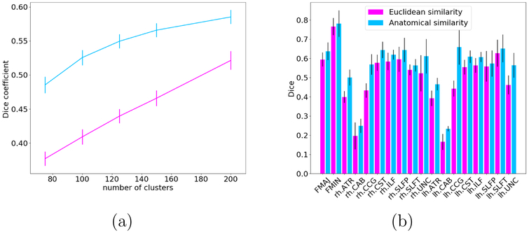
Fig. 4(a) shows the Dice coefficient between the manually labeled WM bundles and the streamline clusters obtained with each of the two similarity measures, averaged over all 18 bundles and 32 subjects, as a function of the total number of clusters. Fig. 4(b) shows the average Dice coefficient over all subjects for each WM bundle, when the total number of clusters is 200. The anatomical similarity measure performed 20% better than the Euclidean similarity measure in terms of its agreement with bundles defined by a human rater. A repeated measures analysis of variance, with factors of similarity measure and number of clusters, showed a statistically significant effect of similarity measure on the Dice coefficient (p < 0.0001).

Figure 4:

(a) Dice coefficient between the manually labeled WM bundles and the streamline clusters obtained with each of the two similarity measures, averaged over all 18 bundles and 32 subjects, as a function of the total number of clusters. (b) Average Dice coefficient over all subjects by tract, when the total number of clusters is 200.

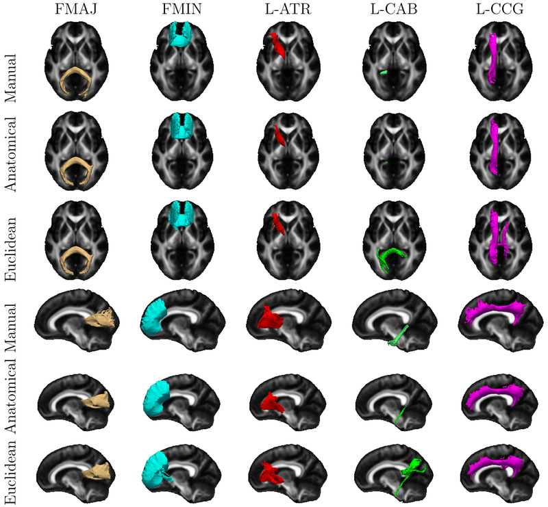
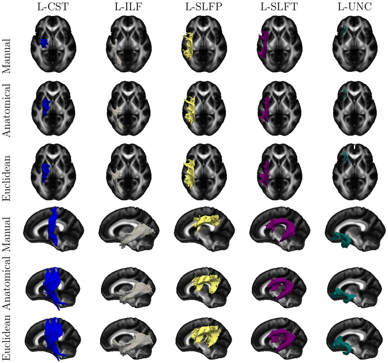
Fig. 5 and Fig. 6 depict the clusters used in the above evaluation, averaged across the 32 subjects in the space of the FMRIB58 FA template (Smith et al., 2006) and displayed as isosurfaces. (Note that we mapped clusters to this template only for the purposes of this illustration. Otherwise, all computations were performed in the native dMRI space of each individual.) For reference, the figures also show population averages of the corresponding manually labeled bundles. Although individual variability and finer differences between methods cannot be appreciated from these population averages, the figures suggest that the 5% threshold that we use to select the clusters included in this evaluation is reasonable.

Figure 5:

Population averages of the manually labeled bundles and the streamline clusters that contain more than 5% streamlines overlapping with the corresponding manually labeled bundle. Each color represents a different WM pathway. The population averages across all subjects are shown as isosurfaces in axial and sagittal views.

Figure 6:

Population averages of the manually labeled bundles and the streamline clusters that contain more than 5% streamlines overlapping with the corresponding manually labeled bundle (continued from Fig. 5). Each color represents a different WM pathway. The population averages across all subjects are shown as isosurfaces in axial and sagittal views.

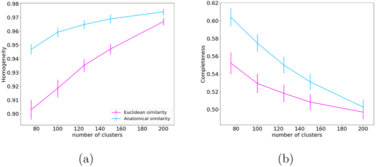
Fig. 7 shows plots of homogeneity (a) and completeness (b) for both the anatomical and Euclidean similarity measure. Our anatomical similarity measure outperforms the Euclidean similarity measure in both homogeneity and completeness. A repeated measures analysis of variance, with factors of similarity measure and number of clusters, showed a statistically significant effect of similarity measure on both homogeneity and completeness (p < 0.0001).

Figure 7:

Homogeneity (a) and completeness (b) of unsupervised clustering, averaged over 18 WM bundles and 32 subjects, as a function of the number of clusters.

We also evaluated a combined similarity measure, summing the anatomical and Euclidean similarities after normalizing them to account for their different variances. We did not find any statistically significant difference between the performance of the combined similarity measure and the anatomical similarity itself (p = 0.85 for Dice coefficient, p = 0.60 for homogeneity, and p = 0.72 for completeness, based on a repeated measures analysis of variance with factors of similarity measure and number of clusters). This suggests that, once the anatomical neighborhood of the streamlines has been taken into account, the spatial coordinates of the streamlines may not contribute additional information to the clustering. Hence, no further results are shown for the combination of similarity measures.

Finally, we evaluated clustering the streamlines after mapping them to the subject’s sMRI space, instead of mapping the cortical parcellation and subcortical segmentation labels to dMRI space. We did not find statistically significant differences between the performance of the anatomical similarity measure in sMRI and dMRI space (p = 0.62 for Dice coefficient, p = 0.55 for homogeneity, and p = 0.9 for completeness, based on a repeated measures analysis of variance with factors the number of clusters and the space that the clustering was performed in). Throughout the paper, the anatomical similarity measure is computed in dMRI space.

3.2. Anatomical and spatial consistency of clusters

Fig. 8(a) shows plots of w_E for clusters derived by optimizing either w_E or w_A. Fig. 8(b) shows plots of w_A for clusters derived by optimizing either w_E or w_A. Finally, Fig. 8(c) shows plots of the mean closest-point distance, w_CP, for clusters derived by optimizing either w_E or w_A.

Figure 8:

Euclidean similarity measure w_E (a), anatomical similarity measure w_A (b), and mean closest-point distance w_Cp (c), for streamlines clustered together either by the Euclidean or the anatomical similarity measure (w_E-optimal vs. w_A-optimal). All measures are plotted as a function of the number of clusters, averaged over all subjects.

Of course we expect that the w_E-optimal clusters have higher wE than the w_A-optimal clusters, and vice versa. This is confirmed in the plots. However, we find that the difference in w_A between the w_E-optimal and w_A-optimal clusters (Fig. 8(b)) is greater than the difference in w_E between the two sets of clusters (Fig. 8(a)). This is confirmed by a repeated measures analysis of variance on these differences, with factors of similarity measure and number of clusters (p < 10⁻⁸). Furthermore, there is no difference in the within-cluster mean closest-point distance between the two sets of clusters (Fig. 8(c)). This is confirmed by a repeated measures analysis of variance on w_CP, with factors of similarity measure and number of clusters (p = 0.3). These results imply that the anatomical similarity measure tends to group together streamlines that are also close to each other in Euclidean space, whereas the Euclidean distance similarity measure may not necessarily yield clusters that are anatomically consistent.

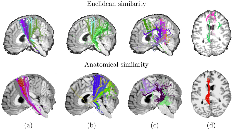
A visual illustration of this is shown in Fig. 9. For four pairs of anatomical segmentation labels, we show the clusters for which at least 5% of streamlines pass through both labels, when the number of clusters is 200. As seen in the figure, the Euclidean distance similarity measure tends to produce noisier and less anatomically consistent clusters than the anatomical similarity measure. For example, streamlines that lie on opposite sides of the midline but are close to each other in space may be erroneously clustered together by w_E, but not by w_A (see Fig. 9(d)).

Figure 9:

Clusters from a single subject, obtained with each of the two similarity measures. Clusters were selected so that at least 5% of the streamlines in a cluster pass through a pair of anatomical segmentation labels: (a) precentral and brainstem, (b) superior parietal and brainstem, (c) superior temporal and precentral, (d) isthmus cingulate and rostral anterior cingulate.

3.3. Robustness to errors in the anatomical segmentation

Fig. 10 shows examples of an original and perturbed segmentation that we used to assess the robustness of the clustering to errors in the boundaries of the anatomical segmentation labels. Fig. 11 shows plots of the Dice coefficient with manually labeled bundles, the homogeneity, and the completeness of the unsupervised clustering, when the original and perturbed segmentations are used to compute the anatomical similarity measure. Based on repeated measures analyses of variance with factors of segmentation type and number of clusters, the effect of the segmentation on the performance measures was not statistically significant (p = 0.79 for Dice coefficient, p = 0.35 for homogeneity, and p = 0.36 for completeness). This suggests that our results are robust to errors in the individual anatomical segmentation.

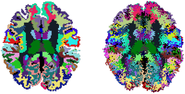
Figure 10:

Example of an original (left) and perturbed (right) indivudual anatomical segmentation used to evaluate robustness to segmentation errors.

Figure 11:

Dice coefficient with respect to manually labeled bundles (a), homogeneity (b), and completeness (c) of unsupervised clustering with our anatomical similarity measure, when the subjects’ original and perturbed anatomical segmentations are used.

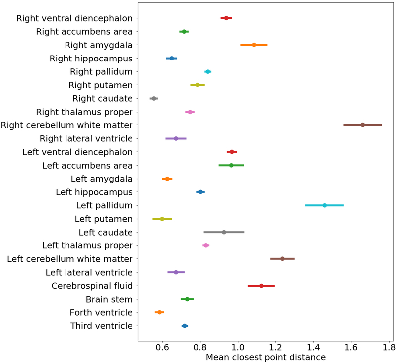
The perturbations that we performed for the above evaluation were in the order of one dMRI voxel. For reference, Fig. 12 shows the accuracy of the automated FreeSurfer segmentation for a set of internal brain structures. The plots show the mean closest-point distance between the automatically segmented and manually labeled structures. The mean error over all structures is 0.9mm, which is less than the sMRI resolution, and much less than the dMRI resolution. Hence, typical FreeSurfer segmentation errors are smaller than the perturbations that we performed in our experiment.

Figure 12:

Mean closest-point distance between automatically segmented and manually labeled brain structures that are included in the FreeSurfer subcortical segmentation.

3.4. Effect of prototype streamlines

Supplemental Fig. S1 shows how the number of prototype streamlines affects the Dice coefficient with manually labeled bundles, the homogeneity, the completeness, and the within-cluster anatomical similarity. As seen in the plots, results obtained with the anatomical similarity measure are very similar for the different numbers of prototype streamlines (50, 100, 250, 500, 1000, 3000). The anatomical similarity measure with 50 prototype streamlines still outperforms the Euclidean distance similarity measure with 500 prototype streamlines (p = 0.002 for Dice and p < 0.0001 for homogeneity and completeness, based on a repeated measures analysis of variance with factors of similarity measure and number of clusters). Supplemental Fig. S2 shows results using 5 different randomly selected sets of 500 prototype streamlines to compute the anatomical similarity measure. For all sets, the anatomical similarity measure outperforms the Euclidean distance similarity measure with 500 prototype streamlines (p < 0.0001 based on a repeated measures analysis of variance with factors of similarity measure and number of clusters). Moreover, the difference between the results obtained with the 5 random sets of prototype streamlines used for the anatomical similarity measure was not significant (p > 0.6 for Dice, homogeneity and completeness, based on a repeated measures analysis of variance with factors of prototype set and number of clusters, for each pair of sets).

3.5. Effect of anatomical neighborhood size

Supplemental Fig. S3 shows how the size of the anatomical neighborhood used for clustering affects the Dice coefficient with manually labeled bundles, the homogeneity, the completeness, and the within-cluster anatomical similarity. Although the 6-element neighborhood leads to somewhat degraded performance, all three anatomical neighborhood sizes perform better than the Euclidean distance similarity measure (p < 0.0001 based on repeated measures analysis of variance with factors of similarity measure and number of clusters).

3.6. Effect of streamline downsampling

Supplemental Fig. S4 shows how downsampling streamlines to N = 10 vs. N = 50 points affects the Dice coefficient with manually labeled bundles, the homogeneity, the completeness, and the within-cluster anatomical similarity. Although the plots show a modest improvement in the Dice coefficient and homogeneity when N = 50 points are used, the difference is not significant (p = 0.1 for Dice coefficient, p = 0.2 for the homogeneity, p = 0.7 for the completeness and p = 0.1 for the anatomical similarity evaluated with repeated measures analysis of variance with factors of similarity measure and number of clusters).

3.7. Comparison to an alternative segmentation

Supplemental Fig. S5 shows results from performing clustering with our anatomical similarity measure, after replacing the subjects’ individual FreeSurfer cortical parcellation and subcortical segmentation with the JHU-ICBM WM atlas. We find that, for the purposes of unsupervised clustering of whole-brain tractography with our anatomical similarity measure, using the individual’s cortical and subcortical labels from FreeSurfer outperforms using labels from a WM atlas (p = 0.0007 for Dice coefficient, and p = 0.0001 for homogeneity and completeness, based on a repeated measures analysis of variance with factors of label set and number of clusters).

3.8. Comparison to shape similarity

Results from the comparison of our anatomical similarity measure to a shape similarity measure are shown in Supplemental Fig. S6. The anatomical similarity measure outperformed the shape similarity measure (p = 0.0003 for Dice coefficient, and p < 0.0001 for homogeneity and completeness, based on a repeated measures analysis of variance with factors of similarity measure and number of clusters). As seen in the figure, the anatomical similarity measure yielded a 30% improvement of the Dice coefficient between clusters and manually labeled WM bundles, when compared to the shape similarity measure.

3.9. Computation time

Table 1 shows computation times for clustering a randomly selected subject’s data with the anatomical and Euclidean distance similarity measure, for six different numbers of prototype streamlines and two different numbers of points per streamline. These times are obtained by assuming that computations of anatomical similarity for different neighborhood elements are parallelized. Otherwise, the computation time for the anatomical similarity measure would also depend on the size of the anatomical neighborhood that is used. Computation is faster for the Euclidean similarity measure when the number of sampled points is small, but it is faster for the anatomical similarity measure when the number of sampled points is large. Note, however, that it would be possible to accelerate computation for the Euclidean similarity measure by parallelizing over the sampled points. Times are reported for a quad-core Xeon 5472 with 3.0GHz CPUs and 7GB of RAM.

Table 1:

Computation times (in minutes) for clustering a randomly selected subject’s data with the two similarity measures and different numbers of prototype streamlines or numbers of points N, assuming that computations of anatomical similarity for different neighborhood elements are parallelized.

Number of prototype streamlines	50	100	250	500	1000	3000
Anatomical similarity (N = 10)	5.31	9.09	21.37	60.07	243.46	1951.30
Euclidean similarity (N = 10)	2.45	4.16	10.14	41.26	282.30	1878.08
Anatomical similarity (N = 50)	8.46	12.57	27.44	74.16	260.20	2347.28
Euclidean similarity (N = 50)	9.20	15.26	36.03	93.29	321.49	2392.37

3.10. Visual illustration

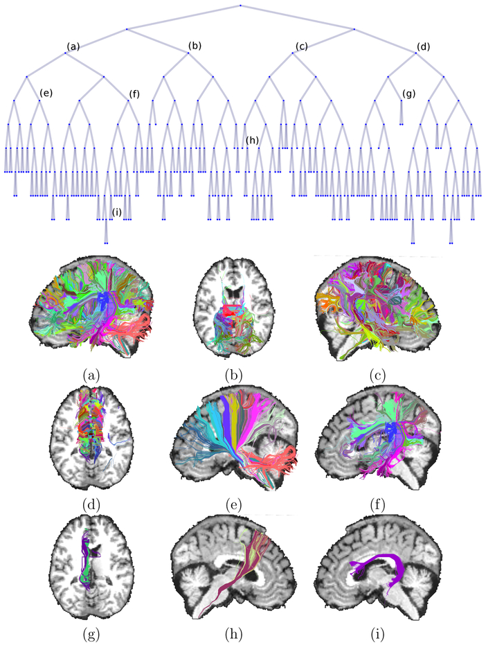
Fig. 13 shows an example of the hierarchical tree generated with the anatomical similarity measure for a randomly selected subject. The root of the tree is the full set of streamlines and the leaves of the tree are the 200 streamline clusters. For a set of nodes that are marked (a)-(i) on the tree, we show images of the clusters at the corresponding iterations of the algorithm:

Figure 13:

Top: Tree representation of the hierarchical cuts performed on a subject’s whole-brain tractography data using our anatomical similarity measure. Bottom: Clusters associated with the tree nodes labeled (a)-(i).

• Low-level nodes represent coarse anatomical divisions of the streamlines: (a) left hemisphere; (b) posterior components of the corpus callosum; (c) right hemisphere; (d) anterior and middle components of the corpus callosum.

• Mid-level nodes represent streamline groupings with greater anatomical specificity: (e) left corticospinal tract and thalamic radiations; (f) left superior longitudinal fasciculus and arcuate fasciculus; (g) left cingulum bundle.

• High-level nodes are individual WM pathways: (h) the right corticospinal tract.

• Leaves (terminal-level nodes) are subdivisions of larger WM pathways: (i) sub-bundle of the left arcuate fasciculus.

In the supplemental material, we provide a video with an example of the tree hierarchy for the anatomical similarity measure. The video shows the left hemisphere clusters, including the subdivisions of the superior longitudinal fasciculus and the arcuate fasciculus.

4. Discussion

In this work we propose a novel anatomical similarity measure for unsupervised clustering of tractography streamlines. Our similarity measure does not use the spatial coordinates of the streamlines, relying instead on histograms of the anatomical segmentation labels that each streamline goes through or next to, at every point along its trajectory. We incorporate this anatomical similarity measure into a divisive hierarchical clustering algorithm, normalized cuts, and compare its performance to that of a conventional similarity measure based on the Euclidean distance between streamlines.

Our results show that streamline clusters obtained with our anatomical similarity measure are in better agreement with WM bundles labeled manually by a trained rater. Specifically, there is a 20% improvement in the overlap with the manually labeled bundles when streamlines where clustered based on their anatomical similarity than their Euclidean distance (Fig. 4). Visual inspection of average clusters across subjects suggests that, when streamlines are clustered based on Euclidean distance, clusters that overlap with these manually labeled bundles include streamlines that are close to the bundles but that would not be assigned to these bundles by a human rater (Fig. 5, Fig. 6). Furthermore, we find that the anatomical similarity measure leads to an increase in both the homogeneity and the completeness of clusters with respect to the manually labeled bundles, when compared to the Euclidean distance-based similarity (Fig. 7). Importantly, the increased agreement between clusters and manually labeled bundles is achieved without introducing any prior information from manual labeling. Our method is unsupervised, using only the subject’s own cortical and subcortical segmentation labels. The improvement stems from the fact that, by not grouping streamlines based on their proximity but based on their anatomical neighborhood, the algorithm follows an approach that resembles the anatomical criteria used by human raters to identify WM bundles.

We also evaluate the anatomical and spatial consistency of clusters obtained by optimizing the anatomical or Euclidean distance similarity measure (Fig. 8). We find that the clusters obtained with the two methods differ significantly more in terms of within-cluster anatomical similarity than they differ in terms of within-cluster Euclidean distance. Furthermore, the within-cluster mean closest-point distance is not significantly different between the clusters obtained with the two methods. This suggests that streamlines that share common anatomical neighbors tend to also be close together in space, but the reverse is not necessarily true (see also Fig.9). It has been pointed out previously that clustering based on spatial coordinates cannot capture all anatomical subdivisions, if the streamlines in the subdivisions do not vary significantly in terms of shape (O’Donnell et al., 2006).

We assess the robustness of our anatomical similarity measure to errors in the anatomical segmentation by repeating the clustering after perturbing the boundaries of the segmentation labels. We find that there is no significant deterioration in the performance of the anatomical similarity measure when the perturbed segmentations are used instead of the original segmentations (Fig. 11). We also show that errors in the automated anatomical segmentation labels obtained by FreeSurfer are smaller than the range of the perturbations performed in our experiment, and smaller than typical dMRI voxel sizes (Fig. 12).

We have chosen to use a randomly selected set of prototype streamlines to compute the similarity matrix at each iteration of the normalized cuts algorithm. This makes computation tractable for the large data sets that result from high-resolution dMRI acquisitions such as the one used here. The number of prototype streamlines has a modest impact on the results, and does not change the conclusions of our performance comparison between similarity measures (Supplemental Fig. S1 and Supplemental Fig. S2). We conclude that a choice of N_p = 500 prototype streamlines is sensible. Note that the number of streamlines to be divided with normalized cuts decreases at each iteration of the algorithm. At the final stages of the clustering (as we get further away from the root of the hierarchical tree of Fig. 13, thus the clusters become finer and greater accuracy becomes crucial), N_p = 500 represents a large portion of the total number of streamlines to be divided.

The number of anatomical neighbors included in our proposed similarity measure is another factor that affects computational complexity, although histogram computations for different neighbors are fully parallelizable. We find a modest improvement in performance when anatomical neighborhoods of size greater than 6 are used (Supplemental Fig. S3), but the anatomical similarity measure outperforms the Euclidean distance similarity measure for any neighborhood size. Finally, for all the results shown here, only long-range connections (streamlines longer than 55mm) are included to reduce computation. Our approach can be applied to full tractography data sets without a reduction in performance at the expense of longer computation times for both similarity measures.

Our evaluation of the anatomical similarity measure after downsampling streamlines to N = 10 vs. N = 50 equispaced points shows that increasing this number may improve results somewhat (Supplemental Fig. S4), although this improvement is not statistically significant. Here we downsampled streamlines to a fixed N for a more balanced comparison to the Euclidean distance similarity measure, which relies on downsampling to reduce computation time. However, our proposed anatomical similarity measure does not require streamlines to have the same number of points, and its computational complexity is not impacted by this number.

We have chosen to compute the anatomical similarity of streamlines with respect to a set of cortical parcellation and subcortical segmentation labels, instead of labels from a WM atlas, for two reasons. First, our goal was to develop an unsupervised method, rather than impose the existence of certain WM bundles through the use of an atlas. Our approach allows exploratory analyses to be performed on tractography data from the whole brain, instead of being limited to a set of pre-defined bundles. Second, our similarity measure relies not only on the structures that a streamline goes through, but also on the structures that surround it, in a set of different directions. Therefore, one might expect a segmentation that includes cortical and subcortical structures to perform well in that setting. Indeed, our results suggest that our anatomical similarity measure works better when we compute it using labels of cortical and subcortical structures, rather than labels from a WM atlas (Supplemental Fig. S5). That is, although a WM atlas can be an extremely valuable tool for supervised reconstruction of specific pathways, it does not appear to be optimal for the purposes of whole-brain tractography clustering based on anatomical similarity.

The similarity measure that we have proposed involves the histograms of the anatomical neighbors of tractography streamlines. These histograms provide an “anatomical signature” that allows us to describe streamlines without relying on their spatial coordinates in a native or template space. We expect this signature to be useful for finding corresponding bundles, e.g., between subjects or between hemispheres, without the need for an exact point-by-point transformation between them. This is an exciting prospect for large population studies, and it will be very important to evaluate our method on larger data sets than the one used here. Early results from applying AnatomiCuts to a much larger set of data from the MGH-Harvard-USC pilot Lifespan Human Connectome Project show promise for using the proposed anatomical similarity measure to find corresponding clusters across subjects aged 8–90 without co-registration (Siless et al., 2017). We intend to investigate this further and to evaluate our method on other large data sets from different disease populations in the future.

In previous work, we used a similar description of the anatomical neighborhood of a path to introduce priors into a global probabilistic tractography algorithm (Yendiki et al., 2011). In that work, histograms of the anatomical neighbors of tractography streamlines were computed from training subjects, where the bundles of interest had been labeled manually, and used as anatomical priors when performing tractography in a novel subject. In the present work, we do not rely on training data; we introduce anatomical information only from the subject’s own anatomical segmentation, and only after the tractography has been performed. On the one hand, this allows us to perform exploratory, whole-brain tractography analyses, without being constrained to a set of bundles included in an atlas. On the other hand, because the tractography is performed in an unconstrained way, it is prone to all the usual errors due to crossing WM bundles, such as streamlines ending prematurely or jumping from one bundle to another. Post hoc clustering methods, like the one presented here, cannot recover from such errors, as they do not modify the tractography streamlines—they only assign the streamlines into groups. It would be possible to use the two approaches in a complementary way. One could apply the unsupervised clustering presented here to high-quality dMRI data (e.g., from the Connectom scanner) to generate clusters from the whole brain, include the clusters that occur consistently across subjects into an atlas to generate priors for the approach in Yendiki et al. (2011), and then apply the latter to reconstruct the same pathways robustly in more routine-quality dMRI data.

5. Conclusion

We present AnatomiCuts, a method for unsupervised hierarchical clustering of dMRI tractography data based on anatomical similarity. We compare this to the conventional approach of using a similarity based on Euclidean distance. We find that the anatomical similarity yields results that are more consistent with manual labeling relative to the Euclidean similarity. That is, without introducing any training data from human raters, we are able to obtain results that are in closer agreement with such a rater. We achieve this simply by using a similarity measure that is better at replicating how a human with neuroanatomical expertise would segment WM tracts, i.e., based on the anatomical structures that they either intersect or neighbor, everywhere along the tracts’ trajectory. This allows us to obtain anatomically meaningful WM bundles without being limited to a set of tracts included in an atlas. Therefore we expect our approach to facilitate fully unsupervised analyses of whole-brain tractography data in large population studies.

References

- Basser PJ, Pajevic S, Pierpaoli C, Duda J, & Aldroubi A 2000. In vivo fiber tractography using DT-MRI data. Magnetic Resonance in Medicine, 44(4), 625–632. [DOI] [PubMed] [Google Scholar]
- Brun A, Knutsson H, Park HJ, Shenton ME, & Westin CF 2004. Clustering Fiber Traces Using Normalized Cuts. International Conference on Medical Image Computing and Computer-Assisted Intervention, 3216/2004(3216), 368–375. [DOI] [PMC free article] [PubMed] [Google Scholar]
- Corouge I, Gouttard S, & Gerig G 2004. (April). Towards a shape model of white matter fiber bundles using diffusion tensor MRI. Pages 344–347 Vol. 1 of: 2004 2nd IEEE International Symposium on Biomedical Imaging: Nano to Macro (IEEE Cat No. 04EX821). [Google Scholar]
- Dice LR 1945. Measures of the Amount of Ecologic Association Between Species. Ecology, 26(3), 297–302. [Google Scholar]
- Ding Z, Gore JC, & Anderson AW 2003. Classification and quantification of neuronal fiber pathways using diffusion tensor MRI. Magnetic Resonance in Medicine, 49(4), 716–721. [DOI] [PubMed] [Google Scholar]
- Fan Q, Witzel T, Nummenmaa A, Van Dijk KRA, Van Horn JD, Drews MK, Somerville LH, Sheridan MA, Santillana RM, Snyder J, Hedden T, Shaw EE, Hollinshead MO, Renvall V, Zanzonico R, Keil B, Cauley S, Polimeni JR, Tisdall D, Buckner RL, Wedeen VJ, Wald LL, Toga AW, & Rosen BR 2016. MGH-USC Human Connectome Project datasets with ultra-high b-value diffusion MRI. NeuroImage, 124, 1108–1114. [DOI] [PMC free article] [PubMed] [Google Scholar]
- Fischl B, Salat David H., Busa E, Albert M, Dieterich M, Haselgrove C, Van Der Kouwe A, Killiany R, Kennedy D, Klaveness S, Montillo A, Makris N, Rosen B, & Dale AM 2002. Whole brain segmentation: Automated labeling of neuroanatomical structures in the human brain. Neuron, 33(3), 341–355. [DOI] [PubMed] [Google Scholar]
- Fischl B, Van Der Kouwe A, Destrieux C, Halgren E, Ségonne F, Salat H, Busa E, Seidman LJ, Goldstein J, Kennedy D, Caviness V, Makris N, Rosen B, & Dale AM 2004. Automatically Parcellating the Human Cerebral Cortex. Cerebral Cortex, 14(1), 11–22. [DOI] [PubMed] [Google Scholar]
- Garyfallidis E, Brett M, Correia MM, Williams GB, & Nimmo-Smith I 2012. QuickBundles, a Method for Tractography Simplification. Frontiers in neuroscience, 6(December), 175. [DOI] [PMC free article] [PubMed] [Google Scholar]
- Gerig G, Gouttard S, & Corouge I 2004. Analysis of brain white matter via fiber tract modeling. Pages 4421–4424 of: Engineering in Medicine and Biology Society, 2004. IEMBS ’04. 26th Annual International Conference of the IEEE, vol. 2. [DOI] [PubMed] [Google Scholar]
- Golub GH, & Van Loan CF 1996. Matrix Computations. [Google Scholar]
- Greve DN, & Fischl B 2009. Accurate and robust brain image alignment using boundary-based registration. Neurolmage, 48(1), 63–72. [DOI] [PMC free article] [PubMed] [Google Scholar]
- Guevara P, Poupon C, Rivière D, Cointepas Y, Descoteaux M, Thirion B, & Mangin JF 2011. Robust clustering of massive tractography datasets. Neurolmage, 54(3), 1975–1993. [DOI] [PubMed] [Google Scholar]
- Guevara P, Duclap D, Poupon C, Marrakchi-Kacem L, Fillard P, Le Bihan D, Leboyer M, Houenou J, & Mangin JF 2012. Automatic fiber bundle segmentation in massive tractography datasets using a multi-subject bundle atlas. Neurolmage, 61(4), 1083–1099. [DOI] [PubMed] [Google Scholar]
- Guha S, Rastogi R, & Shim K 2001. CURE: An efficient clustering algorithm for large databases. Information Systems, 26(1), 35–58. [Google Scholar]
- Hua K, Zhang J, Wakana S, Jiang H, Li X, Reich DS, Calabresi PA, Pekar JJ, Van Zijl PCM, & Mori S 2008. Tract probability maps in stereotaxic spaces: Analyses of white matter anatomy and tract-specific quantification. Neurolmage, 39(1), 336 – 347. [DOI] [PMC free article] [PubMed] [Google Scholar]
- Jenkinson M, Beckmann CF, Behrens TEJ, Woolrich MW, & Smith SM 2012. FSL. [DOI] [PubMed] [Google Scholar]
- Jin Y, Shi Y, Zhan L, Gutman BA, de Zubicaray GI, McMahon KL, Wright MJ, Toga AW, & Thompson PM 2014. Automatic clustering of white matter fibers in brain diffusion MRI with an application to genetics. Neurolmage, 100, 75–90. [DOI] [PMC free article] [PubMed] [Google Scholar]
- Le Bihan D, Breton E, Lallemand D, Grenier P, Cabanis E, & Laval-Jeantet M 1986. MR imaging of intravoxel incoherent motions: application to diffusion and perfusion in neurologic disorders. Radiology, 161, 401–407. [DOI] [PubMed] [Google Scholar]
- Lehman JF, Greenberg BD, McIntyre CC, Rasmussen SA, & Haber SN 2011. Rules ventral prefrontal cortical axons use to reach their targets: implications for diffusion tensor imaging tractography and deep brain stimulation for psychiatric illness. Journal of Neuroscience, 31(28), 10392–10402. [DOI] [PMC free article] [PubMed] [Google Scholar]
- Li H, Xue Z, Guo L, Liu T, Hunter J, & Wong STC 2010. A hybrid approach to automatic clustering of white matter fibers. Neuroimage, 49(2), 1249 – 1258. [DOI] [PubMed] [Google Scholar]
- Maddah M, Zöllei L, Grimson WEL, Westin CF, & Wells WM 2008. A mathematical framework for incorporating anatomical knowledge in DT-MRI analysis. Pages 105–108 of: 2008 5th IEEE International Symposium on Biomedical Imaging: From Nano to Macro, Proceedings, ISBI. [DOI] [PMC free article] [PubMed] [Google Scholar]
- Makris N, & Pandya DN 2008. The extreme capsule in humans and rethinking of the language circuitry. Brain Structure and Function, 213(3), 343–358. [DOI] [PMC free article] [PubMed] [Google Scholar]
- Moberts B, Vilanova A, & Van Wijk JJ 2005. (October). Evaluation of fiber clustering methods for diffusion tensor imaging. Pages 65–72 of: Visualization, 2005. VIS 05. IEEE. [Google Scholar]
- Mori S, Crain BJ, Chacko VP, & Zijl PV 1999. Three-dimensional tracking of axonal projections in the brain by magnetic resonance imaging. Ann. Neurol, 45(2), 265–9. [DOI] [PubMed] [Google Scholar]
- Mugler JP, & Brookeman JR 1990. Three-dimensional magnetization-prepared rapid gradient-echo imaging (3D MP RAGE). Magnetic Resonance in Medicine, 15(1), 152–157. [DOI] [PubMed] [Google Scholar]
- O’Donnell L, Kubicki M, Shenton ME, Dreusicke M, Grimson WEL, & Westin CF 2006. A Method for Clustering White Matter Fiber Tracts. AJNR, 27(5), 1032–1036. [PMC free article] [PubMed] [Google Scholar]
- O’Donnell LJ, & Westin CF 2007. Automatic tractography segmentation using a high-dimensional white matter atlas. IEEE Transactions on Medical Imaging, 26(11), 1562–1575. [DOI] [PubMed] [Google Scholar]
- Oishi K, Faria AV, Van Zijl PCM, & Mori S 2010. MRI Atlas of Human White Matter. Academic Press. [Google Scholar]
- Ros C, Güllmar D, Stenzel M, Mentzel HJ, & Reichenbach JR 2013. Atlas-guided cluster analysis of large tractography datasets. PLoS ONE, 8(12). [DOI] [PMC free article] [PubMed] [Google Scholar]
- Rosenberg A, & Hirschberg J 2007. V-measure: A conditional entropy-based external cluster evaluation measure. Pages 410–420 of: Proceedings of the Joint Conference on Empirical Methods in Natural Language Processing and Computational Natural Language (EMNLP-CoNLL’07), vol.1. [Google Scholar]
- Sammut C, & Webb GI (eds). 2017. Classification Algorithms. Boston, MA: Springer US; Pages 208–209. [Google Scholar]
- Setsompop K, Kimmlingen R, Eberlein E, Witzel T, Cohen-Adad J, McNab JA, Keil B, Tisdall MD, Hoecht P, Dietz P, Cauley SF, Tountcheva V, Matschl V, Lenz VH, Heberlein K, Potthast A, Thein H, Van Horn J, Toga A, Schmitt F, Lehne D, Rosen BR, Wedeen V, & Wald LL 2013. Pushing the limits of in vivo diffusion MRI for the Human Connectome Project. Neuroimage, 80, 220–233. [DOI] [PMC free article] [PubMed] [Google Scholar]
- Shi J, & Malik J 2000. Normalized cuts and image segmentation. IEEE Transactions on Pattern Analysis and Machine Intelligence, 22(8), 888–905. [Google Scholar]
- Siless V, Medina S, Varoquaux G, & Thirion B 2013. (June). A Comparison of Metrics and Algorithms for Fiber Clustering. Pages 190–193 of: 2013 International Workshop on Pattern Recognition in Neuroimaging. [Google Scholar]
- Siless V, Chang K, Fischl B, & Yendiki A 2016. Hierarchical Clustering of Tractography Streamlines Based on Anatomical Similarity Pages 184–191 of: Medical Image Computing and Computer-Assisted Intervention. Springer International Publishing. [Google Scholar]
- Siless V, Davidow JY, Nielsen J, Fan Q, Hedden T, Hollinshead M, Bustamante CV, Drews MK, Van Dijk KRA, Sheridan MA, Buckner RL, Fischl B, Somerville L, & Yendiki A 2017. Registration-free analysis of diffusion MRI tractography data across subjects through the human lifespan. In: Proc. Intl. Soc. Mag. Reson. Med, vol. 25. [Google Scholar]
- Smith SM, Jenkinson M, Johansen-Berg H, Rueckert D, Nichols TE, Mackay CE, Watkins KE, Ciccarelli O, Cader MZ, Matthews PM, & Behrens TEJ 2006. Tract-based spatial statistics: Voxelwise analysis of multi-subject diffusion data. NeuroImage, 31(4), 1487–1505. [DOI] [PubMed] [Google Scholar]
- Sørensen TJ 1948. A method of establishing groups of equal amplitude in plant sociology based on similarity of species and its application to analyses of the vegetation on Danish commons. Biol. Skr, 5, 1–34. [Google Scholar]
- Tsai A, Westin CF, Hero AO, & Willsky AS 2007. Fiber tract clustering on manifolds with dual rooted-graphs. In: Proceedings of the IEEE Computer Society Conference on Computer Vision and Pattern Recognition. [Google Scholar]
- Tunc B, Parker WA, Ingalhalikar M, & Verma R 2014. Automated tract extraction via atlas based adaptive clustering. NeuroImage, 102(P2), 596–607. [DOI] [PMC free article] [PubMed] [Google Scholar]
- Van der Kouwe A, Benner T, Salat DH, & Fischl B 2008. Brain morphometry with multiecho MPRAGE. NeuroImage, 40(2), 559–569. [DOI] [PMC free article] [PubMed] [Google Scholar]
- Visser E, Nijhuis EHJ, Buitelaar JK, & Zwiers MP 2011. Partition-based mass clustering of tractography streamlines. NeuroImage, 54(1), 303–312. [DOI] [PubMed] [Google Scholar]
- Wakana S, Caprihan A, Panzenboeck MM, Fallon JH, Perry M, Gollub RL, Hua K, Zhang J, Jiang H, Dubey P, Blitz A, van Zijl P, & Mori S 2007. Reproducibility of quantitative tractography methods applied to cerebral white matter. NeuroImage, 36(3), 630–644. [DOI] [PMC free article] [PubMed] [Google Scholar]
- Wang Q, Yap PT, Wu G, & Shen D 2013. Application of neuroanatomical features to tractography clustering. Human Brain Mapping, 34(9), 2089–2102. [DOI] [PMC free article] [PubMed] [Google Scholar]
- Wang X, Grimson WEL, & Westin CF 2011. Tractography segmentation using a hierarchical Dirichlet processes mixture model. NeuroImage, 54(1), 290–302. [DOI] [PMC free article] [PubMed] [Google Scholar]
- Wassermann D, Bloy L, Kanterakis E, Verma R, & Deriche R 2010. Unsupervised white matter fiber clustering and tract probability map generation: Applications of a Gaussian process framework for white matter fibers. NeuroImage, 51(1), 228–241. [DOI] [PMC free article] [PubMed] [Google Scholar]
- Wassermann D, Makris N, Rathi Y, Shenton M, Kikinis R, Kubicki M, & Westin CF 2016. The white matter query language: a novel approach for describing human white matter anatomy. Brain Structure and Function, 221(9), 4705–4721. [DOI] [PMC free article] [PubMed] [Google Scholar]
- Wright SM, & Wald LL 1997. Theory and application of array coils in MR spectroscopy. NMR in Biomedicine, 10(8), 394–410. [DOI] [PubMed] [Google Scholar]
- Wu X, Xie M, Zhou J, Anderson AW, Gore JC, & Ding Z 2012. Globally optimized fiber tracking and hierarchical clustering – a unified framework. Magnetic resonance imaging, 30(4), 485–495. [DOI] [PMC free article] [PubMed] [Google Scholar]
- Xia Y, Turken U, Whitfield-Gabrieli SL, & Gabrieli JD 2005. Knowledge-Based Classification of Neuronal Fibers in Entire Brain. Berlin, Heidelberg: Springer Berlin Heidelberg; Pages 205–212. [DOI] [PubMed] [Google Scholar]
- Yeh FC, Wedeen VJ, & Tseng WYI 2010. Generalized q-sampling imaging. IEEE Transactions on Medical Imaging, 29(9), 1626–1635. [DOI] [PubMed] [Google Scholar]
- Yeh FC, Verstynen TD, Wang Y, Fernández-Miranda JC, & Tseng WYI 2013. Deterministic diffusion fiber tracking improved by quantitative anisotropy. PLoS ONE, 8(11). [DOI] [PMC free article] [PubMed] [Google Scholar]
- Yendiki A, Panneck P, Srinivasan P, Stevens A, Zöllei L, Augustinack J, Wang R, Salat D, Ehrlich S, Behrens T, Jbabdi S, Gollub R, & Fischl B 2011. Automated Probabilistic Reconstruction of White-Matter Pathways in Health and Disease Using an Atlas of the Underlying Anatomy. Frontiers in Neuroinformatics, 5, 23. [DOI] [PMC free article] [PubMed] [Google Scholar]
- Zhang T, Chen H, Guo L, Li K, Li L, Zhang S, Shen D, Hu X, & Liu T 2014. Characterization of U-shape streamline fibers: Methods and applications. Medical Image Analysis, 18(5), 795–807. [DOI] [PMC free article] [PubMed] [Google Scholar]
- Ziyan U, Sabuncu MR, Grimson WEL, & Westin CF 2009. Consistency clustering: A robust algorithm for group-wise registration, segmentation and automatic atlas construction in diffusion MRI. Pages 279–290 of: International Journal of Computer Vision, vol. 85. [DOI] [PMC free article] [PubMed] [Google Scholar]
Associated Data
This section collects any data citations, data availability statements, or supplementary materials included in this article.