Data-Driven Investment Strategies for Peer-to-Peer Lending: A Case Study for Teaching Data Science

Abstract

We develop a number of data-driven investment strategies that demonstrate how machine learning and data analytics can be used to guide investments in peer-to-peer loans. We detail the process starting with the acquisition of (real) data from a peer-to-peer lending platform all the way to the development and evaluation of investment strategies based on a variety of approaches. We focus heavily on how to apply and evaluate the data science methods, and resulting strategies, in a real-world business setting. The material presented in this article can be used by instructors who teach data science courses, at the undergraduate or graduate levels. Importantly, we go beyond just evaluating predictive performance of models, to assess how well the strategies would actually perform, using real, publicly available data. Our treatment is comprehensive and ranges from qualitative to technical, but is also modular—which gives instructors the flexibility to focus on specific parts of the case, depending on the topics they want to cover. The learning concepts include the following: data cleaning and ingestion, classification/probability estimation modeling, regression modeling, analytical engineering, calibration curves, data leakage, evaluation of model performance, basic portfolio optimization, evaluation of investment strategies, and using Python for data science.

Goals and Structure

The main goal of this article is to present a comprehensive case study based on a real-world application that can be used in the context of a data science course.^* Teaching data science and machine learning concepts based on a concrete business problem makes the learning process more real, relevant, and exciting, and allows students to understand directly the applicability of the material. While case studies are common practice in many business disciplines (e.g., Marketing and Strategy), it is difficult to find comprehensive case studies to support data science courses, especially cases that span from raw data to actual business outcomes. This article helps to fill this gap. We hope that other authors will continue this effort and develop additional comprehensive teaching cases tailored to data science courses. This is especially important as these topics are increasingly taught to less technical student populations, such as MBA students, who tend to be skeptical of contrived case studies without strong roots in a real business problem.

We chose online peer-to-peer lending as our application for several reasons. First, this is an application area that most people can easily relate to. Second, beyond the use of predictive models, we can also develop prescriptive tools (in this context, investment strategies) so we can directly observe the potential business impact of our models. Third, as discussed in the Story Line section, the largest two online U.S. platforms make their data publicly available, allowing readers to easily reproduce and extend our results.

This article is structured as follows. In the Story Line section, we present the story and background used in our case study. This part motivates the concrete business problem and can be assigned to students before the first class. The Questions and Teaching Material section lists a series of questions that can be used as a basis for in-class discussion, and provides solutions and teaching notes. We divide our treatment into six parts: Introduction and Objectives, Data Ingestion and Cleaning, Data Exploration, Predictive Models for Default, Investment Strategies, and Optimization. The analysis is comprehensive: it describes the entire beginning-to-end process that includes several important concepts such as working with real-data, predictive modeling, machine learning, and optimization. Depending on the needs of the instructor and the focus of the course, these parts can be used independently of each other as needed. Finally, the details of the data used in this case study and a brief description of the structure of the supplemental Jupyter notebooks containing the code are relegated to the Appendix.

This case is intended to complement other teaching resources for data science classes. We do not attempt to teach all the fundamental concepts and algorithms, nor implementation details. For those not familiar with all the concepts in the case, just about all of the data science concepts, including their relationship to similar business problems, are covered in Provost and Fawcett.¹ Using Python for data science and machine learning is covered in McKinney² and in Raschka and Mirjalili.³ Finally, a comprehensive introduction to the theory and practice of convex optimization can be found in Boyd and Vandenberghe.⁴

Story Line

In this case, we follow Jasmin Gonzales, a young professional looking to diversify her investment portfolio.^† Jasmin graduated with a Masters in Data Science, and after four successful years as a product manager in a tech company, she has managed to save a sizable amount of money. She now wants to start diversifying her savings portfolio. So far, she has focused on traditional investments (stocks, bonds, etc.) and she now wants to look further afield.

One asset class she is particularly interested in is peer-to-peer loans issued on online platforms. The high returns advertised by these platforms seem to be an attractive value proposition, and Jasmin is especially excited by the large amount of data these platforms make publicly available. With her data science background, she is hoping to apply machine learning tools to these data to come up with lucrative investment strategies. In this case, we follow Jasmin as she develops such an investment strategy.

Background on peer-to-peer lending

Peer-to-peer lending refers to the practice of lending money to individuals (or small businesses) via online services that match anonymous lenders with borrowers. Lenders can typically earn higher returns relative to savings and investment products offered by banking institutions. However, there is of course the risk that the borrower defaults on his or her loan.

Interest rates are usually set by an intermediary platform on the basis of analyzing the borrower's credit (using features such as FICO score, employment status, annual income, debt-to-income ratio, number of open credit lines). The intermediary platform generates revenue by collecting a one-time fee on funded loans (from borrowers) and by charging a loan servicing fee to investors.

The peer-to-peer lending industry in the United States started in February 2006 with the launch of Prosper,^‡ followed by LendingClub.^§ In 2008, the Securities and Exchange Commission (SEC) required that peer-to-peer companies register their offerings as securities, pursuant to the Securities Act of 1933. Both Prosper and LendingClub gained approval from the SEC to offer investors notes backed by payments received on the loans.

By June 2012, LendingClub was the largest peer-to-peer lender in the United States based on issued loan volume and revenue, followed by Prosper.^** In December 2015, LendingClub reported that $15.98 billion in loans had been originated through its platform. With very high year-over-year growth, peer-to-peer lending has been one of the fastest growing investments. According to InvestmentZen, as of May 2017, the interest rates range from 6.7% to 22.8%, depending on the loan term and the rating of the borrower, and default rates vary between 1.3% and 10.6%.^††

LendingClub issues loans between $1,000 and $40,000 for a duration of either 36 or 60 months. As mentioned, the interest rates for borrowers are determined based on personal information such as credit score and annual income. A screenshot of the LendingClub home page is shown in Figure 1. In addition, LendingClub categorizes its loans using a grading scheme (grades A, B, C, D, E, F, and G where grade A corresponds to the loans judged to be “safest” by LendingClub). Individual investors can browse loan listings online before deciding which loans(s) to invest in (Fig. 2). Each loan is split into multiples of $25, called notes (e.g., for a $2,000 loan, there will be 80 notes of $25 each). Investors can obtain more detailed information on each loan by clicking on the loan—Figure 3 shows an example of the additional information available for a given loan. Investors can then purchase these notes in a similar manner to “shares” of a stock in an equity market. Of course, the safer the loan the lower the interest rate, and so investors have to balance risk and return when deciding which loans to invest in.

FIG. 1.

Screenshot of the LendingClub home page.

FIG. 2.

Example of loan listings (source: LendingClub website, date accessed: May 2018).

FIG. 3.

Example of a detailed loan listing, for a grade A loan. Information available to investors includes the length of the borrower's employment, the borrower's credit score range, and their gross income, among others (source: LendingClub website, date accessed: July 2018).

One of the interesting features of the peer-to-peer lending market is the richness of the historical data available. The two largest U.S. platforms (LendingClub and Prosper) have chosen to give free access to their data to potential investors. This raises a whole host of questions for investors such as Jasmin:

• Are these data valuable when selecting loans to invest in?

• How could an investor use these data to develop tools to guide investment decisions?

• What is the impact of using data-driven tools on the portfolio performance relative to ad hoc investment strategies?

• What average returns can an investor expect from informed investments in peer-to-peer loans?

The goal of this case study is to provide answers to the questions above. In particular, we investigate how data analytics and machine learning tools can be used in the context of peer-to-peer lending investments. We use the historical data from loans that were issued on LendingClub between January 2009 and November 2017.

Data sets and descriptive statistics

As mentioned, the data sets from LendingClub (and Prosper) are publicly available online.^‡‡ These data sets contain comprehensive information on all loans issued between 2007 and the third quarter of 2017 (a new updated data set is made available every quarter). The data set includes hundreds of features, including the following, for each loan:

• 1.Interest rate
• 2.Loan amount
• 3.Monthly installment amount
• 4.Loan status (e.g., fully paid, default, charged-off)
• 5.Several additional attributes related to the borrower such as type of house ownership, annual income, monthly FICO score, debt-to-income ratio, and number of open credit lines.

The data set used in this case study contains more than 750,000 loan listings with a total value exceeding $10.7 billion. In this data set, 99.8% of the loans were fully funded (at LendingClub, partially funded loans are issued only if the borrower agrees to receive a partial loan). Note that there is a significantly larger number of listings starting from 2016 relative to previous years.

The definition of each loan status is summarized in Table 1. Current refers to a loan that is still being reimbursed in a timely manner. Late corresponds to a loan on which a payment is between 16 and 120 days overdue. If the payment is delayed by more than 121 days, the loan is considered to be in Default. If LendingClub has decided that the loan will not be paid off, then it is given the status of Charged-Off.^§§

Table 1.

Loan statuses in LendingClub

Number of days past due	Status
0	Current
16–120	Late
121–150	Default
150+	Charged-off

These dynamics imply that 5 months after the term of each loan has ended, every loan ends in one of two LendingClub states—fully paid or charged-off.^*** We call these two statuses fully paid and defaulted, respectively, and we refer to a loan that has reached one of these statuses as expired.

One way to simplify the problem is to consider only loans that have expired at the time of analysis. For example, for an analysis carried out in April 2018, this implies looking at all 36-month loans issued on or before October 31, 2014 and all 60-month loans issued on or before October 31, 2012.

As illustrated in Figure 4, a significant portion (13.5%) of loans ended in Default status; depending on how much of the loan was paid back, these loans might have resulted in a significant loss to investors who had invested in them. The remainder was Fully Paid—the borrower fully reimbursed the loan's outstanding balance with interest, and the investor earned a positive return on his or her investment. Therefore, to avoid unsuccessful investments, our goal is to estimate which loans are more (resp. less) likely to default and which will yield low (resp. high) returns. To address this question, we investigate several machine learning tools and show how one can use historical data to construct informed investment strategies.

FIG. 4.

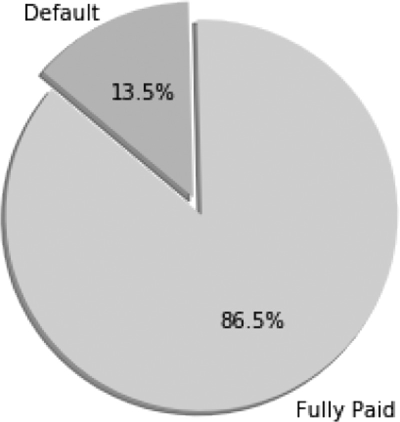
Proportion of Fully Paid versus Default for terminated loans (by November 2017).

Investment strategies and portfolio construction

Making predictions and constructing a portfolio in the context of online peer-to-peer lending can be challenging. The volume of data available provides an opportunity to develop sophisticated data-driven methods. In practice, an investor such as Jasmin would seek to construct a portfolio with the highest possible return, subject to constraints imposed by her risk tolerance, budget, and diversification requirements (e.g., no more than 25% of loans with grades E or F). In this case study, we investigate the extent to which using predictive models can increase portfolio performance.

On important thing that Jasmin will encounter, as in many real applications of predictive analytics, is that it is far from trivial to progress from building a predictive model to using the model to make intelligent decisions. In her prior classes, Jasmin's exercises often ended with estimating the predictive ability of models on out-of-sample data. She will do that here as well—but then she will have to figure out how to estimate the return to expect from an investment. She will find that even with a seemingly good predictive model in hand, estimating the return of an investment requires additional analysis.

Questions and Teaching Material

In this section, we present a number of teaching plans, each of which introduces certain data science concepts in the context of the case study presented in the Story Line section. We divide our analysis into six parts: Introduction and Objectives, Data Ingestion and Cleaning, Data Exploration, Predictive Models for Default, Investment Strategies, and Optimization. Each part is self-contained and includes several questions that could be assigned to students. Each question is followed by detailed explanations and pointers for class discussions. Several parts of this section refer to supplementary Jupyter notebooks that can be obtained from the companion website for this case at guetta.com/lc_case, together with additional teaching materials. The details of the data used in this case study and a brief description of the structure of the notebooks are provided in the Appendix.

Part I: Introduction and objectives

In this part of the case study, we begin by taking stock of Jasmin's problem, and create a framework we will later use to solve it.

• 1.Fundamentally, what decisions will Jasmin need to make?

  Solution: We begin with this question to emphasize the importance of grounding any study of a data set in reality. Indeed, the best way to work with a data set will strongly depend on what our ultimate goal is.

  Arguably, there are two decisions Jasmin might need to make here.

  She will first need to decide how much of her money to invest in LendingClub, and how much to allocate to other options for investment. This would, of course, also require data about her other options. We are not considering this decision in this case.

  Then, once she has decided how much to invest in LendingClub, she will need to decide the exact loans in which to invest her budget. This is the decision we focus on.

  We note that depending on which of the two decisions Jasmin needs to make, her data requirements will be different, as will the techniques she might use.

• 2.What is Jasmin's objective when making these decisions? How will she be able to distinguish “better” decisions from “worse” ones?

  Solution: For this case, we consider this problem to have a clear and simple objective—to make as much money as possible.

  A discussion here should begin with a general description of what this kind of performance evaluation would look like. Conceptually, this is not too difficult—Jasmin should split her data into two parts. She should use the first part to make her decisions, and the second to evaluate them. Specifically, her decisions will be which loans in the second part to invest in, and evaluating her decision will require looking at the actual outcome of those loans and seeing how much money they returned.

  Students may be tempted to end the conversation here. This is an excellent place to emphasize that things can sometimes sound very simple, but can be fiendishly difficult when the details are considered. In particular, in this case, it is difficult to calculate exactly “how much money” a given set of loans will return. Consider, for example, the following:

  • Some loans are 36 months long, and some are 60 months long. Given two loans with the same interest rate and risk profile but different lengths, it is unclear which Jasmin should pick.

  • Clearly, loan defaulting is a bad outcome. However, loans default at different times—some loans will default soon after they are taken out, and some much later. How should Jasmin consider those variations?

  • Some loans might be repaid early, before they expire. This, presumably, is undesirable, since it results in a lost opportunity to earn interest in the remaining period of the loan. However, how should Jasmin take that into account?

  We discuss these issues in greater detail in a later section; for now, students should get the idea that things are not as simple as they look.

  A final complexity involves how to split the data into these two parts. Students might intuit that the data should be split in time for these two parts—we discuss this in more detail later.

• 3.Why would we even think past data would be helpful here? How could Jasmin use past data to help make these decisions?

  Solution: This is, once again, a question that seems simple at first glance, but hides some complexity.

  Conceptually, Jasmin should look at past data and use them to figure out what loan characteristics tend to indicate a loan will be “good.”

  The first implicit assumption here revolves around the decision to look at each loan individually rather than groups of loans. Indeed, if certain groups of loans are correlated to each other, the estimation problem and corresponding strategy will be far more complicated.

  Second, it is unclear what we mean by a “good” loan. There are at least four things Jasmin might want to predict:

  • Whether a loan will default.

  • Whether a loan will be paid back early.

  • If it defaults, how soon will this happen?

  • If it is paid back early, how soon will it be paid back?

  There are, however, other possibilities, for example, combining one or more of these measures. We discuss some of these later. This, of course, is related to the discussion in the previous section.

• 4.Take a look at the data (the student will be asked to download the data in Part II below). Write a high-level description of the different “attributes”—the variables describing the loans. How would you categorize these attributes? Which do you think are most important to an investor such as Jasmin?

  Solution: The idea here is to start talking about the data set, understand the different attributes therein, and potentially engage in a discussion of what the most important attributes might be. It is also an opportunity to emphasize that any discussion of the data set should be grounded in the purpose of looking at the data in the first place (i.e., the points discussed above).

  In particular, a discussion could note the following:

  • Some attributes are related to the borrowers' characteristics (e.g., FICO score, employment status, annual income), others are related to the platform's decisions (e.g., loan grade, interest rate), and the rest are related to the loan performance (e.g., status, total payment).

  • Students might also note that there is some overlap between some of these variables, in that the value of one might inform the value of another (e.g., all else being equal, a defaulted loan is likely to have a lower total payment than a paid off one).

    As mentioned above, the variables relating to return will need to be worked into a form that is useful for our analysis.

  • Some attributes are categorical (e.g., employment status), whereas some others are numeric (e.g., FICO score). The ways to handle categorical and numeric variables are different.

  • Some attributes are constantly updated while some are set once and for all. This is an important point to observe and we discuss it in greater detail in the solution to question 5 (next).

  Finally, the discussion could mention the fact that investors will be most interested in the return on their investments (either actual return or annualized return). Note that there is no variable in the data set with the return information of each loan. Instead, one needs to carefully calculate the return by using the data available (this is far from trivial, as discussed above and in great detail in Part III below). The relevant variables for calculating the return are the loan status, the total payment, the funded amount, the fees generated, and the loan duration.

• 5.When looking through the data, you might have noticed that some of these variables seem related. For example, the total_pymnt variable is likely to be strongly correlated to the loan status. (Why?) Why would this matter, and how would you check?

  Solution: The purpose of this question is to introduce the concept of leakage. Most generally, leakage is a situation in which a model is built using data that will not be available at the time the model will be used to make a prediction. Leakage is particularly insidious when those data give information on the target being predicted. Leakage is a subtle concept and can take myriad forms. This question and the next illustrate two specific examples of leakage in the context of this case, and should provide useful material to discuss the subject.

  This first example illustrates one form of leakage, in which a variable in the data set is highly correlated with the target variable. Training a model using this attribute is likely to lead to a highly predictive model. However, at the time predictions will need to be made (i.e., when deciding which future loans to invest in), these data will not be available.

  In the specific example mentioned here, the total payments made on the loan will trivially be correlated to all four of the measures mentioned above (loan default, loan early repayment, and time of aforementioned events). Indeed, if a loan defaults or is paid back early, total payments on the loan are likely to be lower. Thus, using that variable for prediction will likely result in a strong model performance. However, when investing in future loans, Jasmin would not have access to the total amount that would eventually be repaid on that loan, and thus, a model trained using that variable could not be used to make future predictions.

• 6.Based on the variable names in the data, it is unclear whether the values of these variables are current as of the date the loan was issued, or as of the date the data were downloaded. For example, suppose you download the data in December 2017, and consider the fico_range_low variable for a loan that was issued in January 2015. It is unclear whether the score listed was the score in January 2015, or the score in December 2017. Why would this matter, and how might you check?

  Solution: This is another more general form of the type of leakage observed in the previous question. Many of the variables in the data set are in fact updated over time, and in some cases, the update is highly indicative of the outcome. For example, if a loan defaults, the borrower's FICO score might go down. Thus, for the same reasons as above, using this score in a predictive model would result in overly optimistic results.

  Detecting this form of leakage is difficult given a static data set. High correlation with the target variable is certainly one diagnostic that could be useful. The best method to eliminate leakage is to obtain data from the time point and context in which they would have been used. We may have to simulate this, for example, going back to database files from the point in time where the decision would have been made (which may be different for every decision). Even detecting the possibility of leakage is very difficult. One method is to compare the data from the time point of decision-making with later data, to see what variables have changed. We illustrate this approach below.

Part II: Data ingestion and cleaning

In this part of the case, we ingest the LendingClub data and clean them to make sure they can be used for model fitting.

• 1.Download the LendingClub data set from the LendingClub website and read it into your programming language of choice. You will notice the data are provided in the form of many individual files, each spanning a certain time period. Combine the different files into a single data set.

  Solution: See the ingestion_cleaning notebook.

  The code provided illustrates a few key features of Pandas:

  • Pandas basic abilities for indexing tables, concatenating different tables, and so on.

  • The ability to read from zip files directly without decompressing them.

  • The ability to read comma separated values (CSV) files in which some lines are irrelevant—these lines can simply be skipped.

  When combining the multiple files, the code also carefully

  • ensures the different files have identical formats,

  • ensures each file has the same set of primary keys (loan IDs), and

  • ensures the loan IDs are indeed a unique primary key once the loans are joined.

• 2.Together with this case, you may have received a copy of the data downloaded from the LendingClub website in 2017. If so, compare these two sets of files—does anything appear amiss?

  Solution: This is a practical illustration of the issue of leakage described above. Students might be tempted to use every attribute from the data in their models. Unfortunately, this would be ill-advised, because LendingClub updates some of these variables as time goes by. Thus, many of the variables in the data table will contain data that were not available at the time the loan was issued and therefore should not be used to create an investment strategy.

  As discussed above, one common pitfall that arises in building and assessing predictive models is leakage from a situation in which the value of the target variable is known, back to the setting in which we evaluate the model—where we are pretending that the target variable is not known. This leakage can occur, for example, through another variable correlated with the target variable. Note that leakage is insidious, because it often affects both the training and test data, and so, typical evaluations will give overly optimistic results.

  The notebook contains code that looks at the two sets of files and compares values that may have changed between them. It also ensures that attributes of interest have not changed too much.

  It is interesting to note that the interest_rate variable does change occasionally after the loan is issued. We will eventually get rid of this variable in building our models, so this should not be too worrying, but it is worth noting.

• 3.Remove all instances (in our case, rows in the data table) representing loans that are still current (i.e., that are not in status “Fully Paid,” “Charged-Off,” or “Default”), and all loans that were issued before January 1, 2009. Discuss the appropriateness of these filtering steps.

  Solution: This is straightforward to do (see the notebook), but hides considerable complexity.

  Indeed, looking back at the body of the case, the method we suggested there to select loans was subtly different. We suggested that we should only look at 36-month loans issued before October 2014, and 60-month loans issued before October 2012. This would ensure that all loans in the period selected had expired (although it would introduce a correlation between the issue date of the loan and its length in our data).

  Using the method here instead has two effects:

  • We oversample loans issued earlier—indeed, loans that are issued earlier are more likely to have expired at the time of our analysis. This is less of an issue, for two reasons.

    —LendingClub has grown tremendously over the past few years, and the number of loans issued by the platform has therefore increased. Thus, a time imbalance already exists in our data set regardless.

    —As demonstrated below, our models are remarkably stable across the time horizon considered—models trained on the 2009 data perform just as well on the 2017 data as models trained more recently.

  • We oversample shorter loans—indeed, at any given point in time, the set of all expired loans will by definition contain a larger number of shorter loans (i.e., loans that have expired early).

    This is a more worrisome issue, since shorter loans might be more or less likely to default. This, in turn, might skew our evaluation metrics. Suppose that in our full data set, the average default rate is x%. Adding a greater proportion of shorter loans might change this number. Our evaluation would then be against this new number and might not reflect the actual performance of the model out of sample.

    Nevertheless, discarding these loans would result in our throwing away a large amount of data that could be used to train these models. We therefore keep those loans in this case, but performing the analysis without these loans would form an excellent follow-up exercise.

• 4.Visualize each of the attributes in the file. Are there any outliers? If yes, remove these.

  Solution: This question is an opportunity to demonstrate different visualization methods appropriate for the different attributes. The ingestion_cleaning notebook demonstrates the use of box-and-whisker plots for continuous variables and histograms for discrete variables, but additional methods could also be introduced.

  This data set is also interesting in that many attributes do not have a clear point at which outliers should be cut off. The notebook suggests some cutoff points, but they are by no means the only possible ones.

  An interesting discussion could be around situations in which outliers appear in target variables or in leakage variables (see Question 5 in Part 1 above). Since the values of these variables would not be known at the time of learning or use, removing instances with outlying values in these variables could render the data set unrealistic. For simplicity, we ignore this issue in our analysis.

• 5.Save the resulting data set in a Python “pickle.” For the sake of this case, restrict yourself to the following attributes: id, loan_amnt, funded_amnt, term, int_rate, grade, emp_length, home_ownership, annual_inc, verification_status, issue_d, loan_status, purpose, dti, delinq_2yrs, earliest_cr_line, open_acc, pub_rec, fico_range_high, fico_range_low, revol_bal, revol_util, total_pymnt, and recoveries.

  Solution: This question introduces the use of pickles, a useful tool in Python. In a later question, we discuss the rationale for selecting these specific attributes.

Part III: Data exploration

In this part, we explore the data we cleaned in the previous part.

• 1.The most important data we will need in determining the return of each loan are the total payments that were received on each loan. There are two variables related to this information—total_pymnt and recoveries. Investigate these two variables, and for each loan determine the total payment made on each loan.

  Solution: The purpose of this question (and, indeed, of every question in the data preparation part of this case) is to encourage students to be hypercritical of data they obtain, and to fully understand them before analyzing them.

  In this case, there are two variables of concern—total_pymnt, which presumably contains the total payment made on that loan, and recoveries, which presumably contains any money recovered after the loan defaulted. A question students should come to is: “does the total_pymnt variable include those recoveries, or do they need to be added on”?

  To investigate this matter, an additional data set is required, also available from LendingClub. The data set lists—for every loan—every payment that was made chronologically on that loan. Using this data set, the ingestion_cleaning notebook confirms that the total_pymnt variable does include all payments.

  This question also introduces another important Python concept: the handling of files that are too large to fit in memory. In this case, the detailed payment file is so large that it cannot be loaded all at once on most personal computers; the notebook uses a Pandas iterator to consider the file line-by-line in performing this check.

• 2.A key measure we will need in working out an investment strategy is the return on each loan, defaulted or otherwise. How might you calculate this return? Add this new variable to the data.

  Solution: At first sight, this question appears simple. As mentioned at the outset, in reality, it is anything but. Calculating the return is complicated by two factors: (1) the return should take into account defaulted loans, which usually are partially paid off, and (2) the return should also take into account loans that have been paid early (i.e., before the loan term is completed).

  This issue could lead to an interesting class discussion. A more complex way to handle this task is to build a dynamic model, in which we take into account potential future reinvestments if a loan is repaid early.

  Assuming we want to avoid this complexity, the following three methods are among the most obvious ways to convert this to a static problem. Before we list these methods, we define the following notation:

  • f is the total amount invested in the loan.

  • p is the total amount repaid and recovered from the loan, including monthly repayments, and any recoveries received later.

  • t is the nominal length of the loan in months (i.e., the time horizon the loan was initially issued for; this will be 36 or 60 months).

  • m is the actual length of the loan in months—the number of months from the date the loan was issued to the date the last payment was made.

    Having established this notation, the three methods are as follows:

  • Method 1 (M1—Pessimistic) supposes that, once the loan is paid back, the investor is forced to sit with the money without reinvesting it anywhere else until the term of the loan. In some sense, this is a worst-case scenario—interest is only earned until the loan is repaid, but the investor cannot reinvest.

    Under this assumption, the (annualized) return can be calculated as

    

    The downside of this method is obvious—the assumptions are hardly realistic.

    Note that this method handles defaults gracefully, without artificially blowing up the returns. Indeed, since the investor was initially intending for his or her investment to remain “locked up” for the term of the loan, it is reasonable to spread the resulting loss over that term.

    For loans that go to term (i.e., are not repaid early and do not default), this method also treats long- and short-term loans in the same way. For loans that are repaid early, however, this method favors short-term loans because the gain realized before the loan is repaid is spread over a shorter time span. Similarly, for loans that default early, this method favors long-term loans because the loss is spread out over a greater time span.

  • Method 2 (M2—Optimistic) supposes that, once the loan is paid back, the investor's money is returned and the investor can immediately invest in another loan with exactly the same return.

    In that case, the (annualized) return can easily be calculated as

    

    The upside of this method is that it is simple and takes into account the fact that funds would (or could) be reinvested. The money is indeed returned to the investor after the loan is repaid, and the investor is able to reinvest the cash.

    It is worth noting that this method is equivalent to simply considering the annualized monthly return of the loan over the time it was active, effectively treating a loan that was repaid early and a loan that went to term in the same way.

    There are, however, two drawbacks. The first is the assumption that the cash can be reinvested at the same rate (although the method could be modified to assume the cash can be reinvested at a lower rate—e.g., the prevailing prime rate). The second more worrying drawback is that if a loan defaults early, annualizing the loss can result in a huge overestimate of the negative return. Indeed, if a loan defaults in the first month, the investor loses 100% of the investment. This is the maximum loss, but annualizing it would lead to a 1200% loss—in other words, we would be assuming the investor reinvests in an equally risky loan for the 11 remaining months of the year, each of which defaults in 1 month! Hardly realistic. We therefore use the following two-piece formula:

    

    One last feature worth noting about this method is that it treats short and long notes equally. Indeed, since it is assumed the investor can always reinvest in a note of equal return immediately after this note ends, the actual term of the loan does not matter. Depending on Jasmin's priorities, this could be appropriate, or it could not—in particular, whether this is appropriate will depend on the horizon over which she is planning her investments.

  • Method 3 (M3) considers a fixed time horizon (e.g., T months) and calculates the return on investing in a particular loan under the assumption that any revenues paid out from the loan are immediately reinvested at a yearly rate of i%, compounded monthly, until the T-month horizon is over (throughout this case study, we consider a 5-year horizon, i.e., T = 60).

    The upside of this method is that it is closest to what would realistically happen. It equalizes all differences between loans of different lengths and correctly accounts for defaulted loans. The downside is that it undervalues the time value of money (in reality, some investors would be unlikely to reinvest at the prime rate and more likely to invest in higher grossing securities). Of course, this could be remedied by adapting the value of the rate. (Indeed, if one had an expected rate of return for the group of loans from which the loan in question was drawn, then that return could be used, yielding possibly different projected future investment returns for different loans.)

    Assuming our notation above, and assuming the payouts were made uniformly through the length m of the loan, each monthly payment was of size p/m. Assuming these are immediately reinvested, we can use the sum of a geometric series to find the total return from the f initially invested:

    

    In this case study, we report results for all three methods.

• 3.As discussed in the case, LendingClub assigns a grade to each loan, from A through G. How many loans are in each grade? What is the default rate in each grade? What is the average interest rate in each grade? What about the average percentage (annual) return? Do these numbers surprise you? If you had to invest in one grade only, which loans would you invest in?

  Solution: This is a great opportunity to illustrate aggregation and “group by's” in Python. Here, we also use different definitions of returns as discussed above.

  Unsurprisingly, the lower the grade, the higher the probability of default, and the higher the average interest rate LendingClub charges.

  It is interesting to note the trend in returns for methods M3 as we move from grade A to grade B and so on. In an ideal world, we might expect the returns to be more-or-less identical across grades. Even though default rates are higher for lower grades, the interest rates are much higher—LendingClub raises the interest rates there to make up for this increased chance of default. It is therefore good to see that returns do not drop precipitously for lower grades.

  The fact that returns do eventually drop faster for lower grades implies either that LendingClub might find it harder to set interest rates to exactly offset defaults for those grades (perhaps as a result of increased volatility for lower grade loans), or that our definition of return is different from LendingClub's. As we saw, there are many ways to define return depending on our objective, and it is conceivable that LendingClub's objectives are different from the ones we outline above. The rest of this case focuses specifically on making investment decisions with respect to the objectives highlighted above.

				Mean return
Grade	% of loans	% Default	Av. interest	M1	M2	M3 (1.2%)	M3 (3%)
A	16.68	6.33	7.22	1.66	3.89	2.05	3.71
B	28.86	13.48	10.85	1.58	5.01	2.02	3.68
C	27.99	22.41	14.07	0.62	5.39	1.39	3.02
D	15.44	30.37	17.54	0.05	5.71	0.92	2.51
E	7.59	38.83	20.73	−0.91	5.95	0.11	1.64
F	2.72	44.99	24.47	−1.43	6.43	−0.44	1.05
G	0.73	48.16	27.12	−2.58	6.66	−1.40	0.05

Part IV: Predictive models for default

In this section, we use predictive analytics to predict how likely a loan is to default.

• 1.Using the data provided, implement models to predict the probability each loan defaults. You may want to try the following models: decision tree, random forest, logistic regression ( and penalized), naive Bayes, and multilayer perceptron. Carefully explain how you selected optimal model parameters and how you evaluated each model/modeling procedure.

  Solution: This question provides an excellent opportunity to teach a number of topics:

  • Each of the models mentioned in the question,

  • How each of those models is learned from data,

  • Hyperparameter tuning through cross validation,

  • Model evaluation for classification models, and

  • Nested cross-validation (i.e., making sure that the data used for hyperparameter tuning are not used when measuring the ultimate performance).

  In discussing the evaluation of classification models, the following two important measures could be discussed:

  • How well do the model's estimates of class probability actually order the loans by their likelihood of default? This is measured by the area under the ROC curve (AUC), which is equivalent to the Mann–Whitney–Wilcoxon statistic. Technically, the AUC measures the following. Given two randomly selected loans, one that defaults and one that does not, what is the probability that the model will assign a higher default probability to the defaulting loan? A model that can perfectly discriminate defaults from nondefaults would have an AUC of 1.0.

  • The calibration of the model—the extent to which the probabilities predicted by the model correspond to the frequency of the event happening for some natural grouping of events. Typically, this is measured by considering instances grouped into bins of similar estimated probabilities. Since our goal is to use the probabilities output by the model to calculate/predict the expected return of loans, the calibration of the estimated probabilities is important here. However, note that we really need to look at calibration in tandem with a measure such as AUC—a model that for every example predicted the base rate (the data set or population default frequency, in this case) would be perfectly calibrated and would not discriminate cases at all.

  See the next question for a summary of the results on a more restricted set of features. As an example, using the full set of features in the notebook, learning a random forest (using the procedure specified in the notebook) yields an out-of-sample AUC of 0.70.

  This is also a good place to discuss calibration and associated diagnostics; see the solution for the next question for a discussion of this point.

  One point that bears discussing in more detail is the method used for training, testing, and cross validation. In this instance, there are, at least two methods we could use:

  • Randomly assign each loan to a training set or a testing set. Within the training set, randomly assign loans to one of the folds for K-fold cross-validation.

  • Set a “cutoff” date. Assign all loans that were issued before that date to the training set, and all loans after that date to the evaluation set. Within the training set, create folds using a sliding time window.

  Arguably, the latter method is more appropriate for this case, because it correctly reflects the way the model will in fact be used in practice (trained on an earlier period and then evaluated on a later period). The first method, on the other hand, might be more desirable for two reasons: first, it is simpler to implement using standard libraries; thus, it is likely to be the first method tried by a data scientist, even if she or she were planning to eventually apply the second method. Also, the first method allows many thousands of different train/test sets to be created using different random seeds. This, in turn, can be used to obtain estimates of various errors in the estimated models, as discussed below. This would be difficult to do using the second method. For this reason, we use the random assignment method here. The intrepid student could be encouraged to compare with the second method.

  (NB: To ensure that the first method is not too problematic, we later assess the stability of our models over time by looking at whether a model trained in 2009 performs worse in 2017 than a model trained on more recent data. We find that our model's performance is remarkably stable.)

• 2.After learning and evaluating these models, Jasmin realized that the attributes she used in her models were not all underlying facts about the loan applicants, but possibly statistics calculated by LendingClub using its own models. She wanted to assess whether the predictive power of her models came simply from LendingClub's own models. Carry out this investigation—what are your conclusions?

  Solution: This question provides a good opportunity to discuss the ways information from some attributes can be incorporated in others. Students may be tempted to simply drop the “Grade” attribute and proceed. However, in reality, the attributes describing the interest rate and installment amounts also reflect the grade (the higher the grade, the lower the interest rate and installment amounts).

  Fitting logistic regressions based on grade only, or interest rate only, we obtain models with out-of-sample AUCs of 0.68. Using only these single variables provides just as much predictive power as the entire set of variables involved, as we achieve this same AUC using logistic regression with all the features.

  As mentioned, Jasmin wanted to assess models using the underlying data only, not the attributes derived by LendingClub. Removing these attributes and refitting the models above, we obtain the following performance values (note that these are averages over many different train/test splits—see note 1 below):

  The first interesting observation is that the above classifiers uniformly perform substantially better than random. Logistic regression performing as well (in this sense) as the nonlinear models suggests (i) that interactions between our variables are not crucial in modeling probability of default, or (ii) that we do not have sufficient training data to learn the interactions well, or (iii) the AUC does not reveal the advantage of learning nonlinearities.

  For simplicity going forward, we use random forest in the rest of this case study. The student may be challenged to compare the results using other models.

  There are three additional points that should be highlighted:

  • (a)Examining a model's performance over a single partition of the data into cross-validation folds can be misleading, as it is possible that the partition gives particularly good or bad training/test splits by chance.

    To ensure the robustness of the results, it is advisable to attempt the operations over many cross-validation runs, each using a different seed to generate the partitions and the train/test split. The code provided allows this to be done easily by adjusting the value of the seed. We performed 200 independent iterations with different seeds and reported the average values above. The following violin plots (another technique worth discussing) presented in Figure 5 illustrate the different results obtained with each method:

  • (b)As discussed in the solution to the previous question, the AUC only measures the ranking performance of the model. Another important measure is the calibration, which measures whether probabilities produced by the model are correct. The notebook provided also produces a test of calibration for each model, and random forests also perform particularly well there. In Figure 6, the x-axis corresponds to the default probability predicted by the model and the y-axis represents the actual proportion of defaulted loans in the test set.
• 3.After modifying her model to ensure she did not include data calculated by LendingClub or leakage affecting the target variable, Jasmin wanted to assess the extent to which her scores agreed with the grades assigned by LendingClub. How might she do that?

  Solution: This provides a good opportunity to introduce the idea of rank correlation, and a measure for it such as Kendall's tau coefficient. For most of the models considered, the coefficient is above 0.5, implying a pretty good agreement between the LendingClub's grades and our scores.

• 4.Finally, Jasmin had one last concern. She was acutely aware of the fact the data she was using to train her models dated from as far back as 2009, whereas she was hoping to apply them going forward. She wanted, therefore, to investigate the stability of her models over time. How might she do this?

  Solution: The notebook presents examples of models that are trained over an early period, and evaluated on a later period. The performance is remarkably stable throughout.

• 5.Go back to the original data (before cleaning and attribute selection) and fit a model to predict the default probability using all attributes. (For the sake of simplicity, it will be sufficient to limit yourself to the following attributes: id, loan_amnt, funded_amnt, funded_amnt_inv, term, int_rate, installment, grade, sub_grade, emp_title, emp_length, home_ownership, annual_inc, verification_status, issue_d, loan_status, purpose, title, zip_code, addr_state, dti, total_pymnt, delinq_2yrs, earliest_cr_line, open_acc, pub_rec, last_pymnt_d, last_pymnt_amnt, fico_range_high, fico_range_low, last_fico_range_high, last_fico_range_low, application_type, revol_bal, revol_util, recoveries.) Does anything surprise you about the performance of this model (out-of-sample) compared with the other models you have fit in this section?

  Solution: This question strikingly illustrates the concept of leakage. As mentioned above, a number of variables represent data not available at the time the loan was issued. In all the models constructed thus far, we have carefully removed these attributes. In this question, we reintroduce them (e.g., last_fico_range_high uses the applicant's most recently available FICO score rather than the score at the time the loan was issued).

  Unsurprisingly, using these additional attributes improves the model's performance. What is truly striking is how much they improve it. Using those attributes, we obtain an out-of-sample AUC of over 0.99 (see the implementation and results in the modeling_leakage notebook). Indeed, a number of write-ups of analyses of this data set found online report similar very high performances of their models without any caveats. Guiding students through the process of getting such a high predictive performance and then realizing how misleading the result is could result in a lively class discussion.

  Throughout this case, we have instructed students to keep only certain attributes after cleaning the data; this question provides an opportunity to justify the set of attributes that was selected. Referring back to Figure 3, the set of attributes we chose is precisely the intersection of the attributes that are available at the time of investment, and those attributes in the historical data that are not updated over time. Thus, the model that results is one that could realistically be used by a potential investor such as Jasmin.

FIG. 5.

Comparison of the different classification models.

FIG. 6.

Calibration curves of different classification models: (a) Naive Bayes, (b) logistic regression (Ridge), (c) decision tree, and (d) random forest. Together with each calibration curve, we include histograms representing the total number of data points with each predicted probability. Calibration results are sometimes unstable in regions with very few points. It is interesting to note that (as expected) due to the conditional independence assumption, Naive Bayes is more likely to predict extreme scores.

Model	Out-of-sample AUC
Naive Bayes	0.65
-penalized logistic regression	0.69
-penalized logistic regression	0.69
Decision tree	0.66
Random forest	0.69
Multilayer perceptron	0.69

Part V: Investment strategies

Jasmin was finally ready to start building investment strategies. It is worth noting that there are many potential strategies Jasmin could try. We consider four strategies here, but interest students should be encouraged to try others too.^††† The strategies we consider here are as follows:

• Random strategy (Rand)—randomly picking loans to invest in.

• Default-based strategy (Def)—using the random forest default-predictor models described above. Then, sorting loans by their estimated default probabilities, and selecting the loans with the lowest probabilities.

• Simple return-based strategy (Ret)—training a simple regression (e.g., Lasso, random forest regressor, multilayer perceptron regressor) model to predict the return on loans directly. Then, sorting loans by their predicted returns and selecting the loans with the highest predicted returns.

• Default- and return-based strategy (DefRet)—training two additional models—one to predict the return on loans that did not default, and one to predict the return on loans that did default. Then, using the probability of default predicted by the random forest model above to find the expected value of the return from each future loan. Invest in the loans with the highest expected returns.^‡‡‡

Note that all these strategies make the assumption that if Jasmin decides to invest in a loan, she must invest in the loan in its entirety (i.e., she cannot invest in a fraction of a loan). In reality, LendingClub does allow investors to invest in fractions of loans, and incorporating this additional complexity could further improve her returns.

• 1.First, consider the three regression models described above (regressing against all returns, regressing against returns for defaulted loans, and regressing against returns for nondefaulted loans). In each case, try and penalized linear regression, random forest regression, and multilayer perceptron regression.

  Solution: Again, this section could lead to a discussion of each of these methodologies, as well as whether the evaluation of the regression results using standard metrics gives insight into whether they will be helpful in solving the business problem. The following table and Figure 7 compare the R² scores for these models. Do they perform well? (Again, these numbers are averages over a number of train/test splits.) Can you tell?

• 2. Now, implement each of the investment strategies described above using the best performing regressor. In particular, suppose Jasmin were to invest in 1000 loans using each of the four strategies, what would her returns be?

  Solution: See the notebook for implementation details. The results are presented in the following table (the results are averaged over 200 independent iterations) and in Figure 8. The last row (Best possible) corresponds to the top 1000 performing loans in hindsight, that is, the best 1000 loans Jasmin could have picked.

  In all cases, the two-stage analytical engineering strategy performs best. The following points may be relevant in a class discussion:

  • The random returns are positive in all cases; this is to be expected and indicates that LendingClub does set interest rates to offset the default risk, at least to some degree.

  • In light of the first point, it is especially pleasing to see our methods significantly outperforming random investments—given LendingClub's ability to set interest rate to offset defaults, extracting value through these investments is nontrivial.

  One point worth highlighting here is the fact it is crucial that the loans used in the simulated tests are not the loans that were used in the training set for building the model. The notebook provided ensures that this is indeed the case.

  An additional interesting observation from the plots above is the following:

  • For a given investment strategy (Rand, Def, Ret, DefRet), the return performance improves as the return definition is more optimistic (as expected).

  • Under a given return definition (M1-PESS, M2-OPT, M3), the return performance improves as the investment strategy becomes more sophisticated. The highest performance is obtained for the DefRet strategy.

• 3.How might Jasmin test the stability of these results?

  Solution: See the notebook for implementation details. As described above, we use a variety of train/test splits.

• 4.The strategies above were devised by investing in 1000 loans. Jasmin is worried, however, that the strategy is not scalable—in other words, if she wanted to increase the number of loans she wanted to invest in, she would eventually “run out” of good loans to invest in. Test this hypothesis using the best strategy above.

  Solution: The graph in Figure 9 illustrates the expected return obtained using the M1 return definition and the DefRet strategy (a random forest classifier and a random forest regressor) as a function of the portfolio size (which varies between 1000 and 9000 loans). These results were obtained by running a single run out-of-sample.

  As one can see from Figure 9, the return decreases with the portfolio size. Why is it the case? One explanation is as follows: when the portfolio size increases, the proportion of good performing loans decreases. As a result, it is hard to maintain the same return performance. This observation can also be used to discuss the fact that our analysis here assumes that we can pick any of the historical loans. In practice, however, investors are limited to a small number of available loans at each point in time.

FIG. 7.

Comparison of the different regression models: (a) M1PESS, (b) M2OPT, (c) M3 (1.2%), and (d) M3 (3%).

FIG. 8.

Comparison of the different investment strategies: (a) M1PESS, (b) M2OPT, (c) M3 (1.2%), and (d) M3 (3%).

FIG. 9.

Returns of the DefRet strategy for different portfolio sizes.

	R2 scores for each return definition
Model	M1	M2	M3 (1.2%)	M3 (3%)
regressor	0.026	0.012	0.027	0.027
regressor	0.026	0.013	0.027	0.027
Multilayer perceptron regressor	0.016	0.004	0.017	0.017
Random forest regressor	0.028	0.018	0.029	0.032

	Return calculation method
	M1-PESS, %	M2-OPT, %	M3 (1.2%)	M3 (3%)
Rand	0.6	5.2	1.2	2.7
Def	1.9	5.3	1.4	3.0
Ret	2.6	5.6	1.6	3.2
DefRet	3.0	5.7	1.7	3.3
Best possible	12.0	27.1	10.1	11.7

Part VI: Optimization

In this section, we investigate ways Jasmin might improve her investment strategy using optimization. Can you formulate the investment problem as an optimization model? How does your model perform compared with the best method above? To solve the optimization problem, you can use a solver such as Gurobi or CPLEX (free academic licenses are available). The reference manual for Gurobi is available.⁵

Solution: This part of the case provides an opportunity to teach basic optimization using Python. In addition, it touches on several modeling ideas that could be discussed in class.

We begin by creating a binary variable for every loan in our data set. In particular,

We let r_i denote the predicted expected return of loan i and A_i the loan amount. We let p_i denote the predicted probability loan i will default. Finally, we let N denote the number of loans we want to invest in (i.e., the desired size of the portfolio). Throughout this section, the return we use for r_i is based on M1-PESS.

We begin by formulating a simple integer program equivalent to strategy Def above (i.e., sorting loans by their default probabilities and selecting the loans with the lowest default probabilities):

As we can see from the notebook, this strategy yields a 2.36% return (run over a single training/test split). Note that one could further incorporate several (linear) constraints such as imposing a maximal allowed value for p_i.

Similarly, the strategies in the previous section can all be written in this optimization form. For example, if r_i were computed based on DefRet, we could rewrite this strategy as follows:

This yields a 2.99% return, identical to the return obtained above, as expected.

We now aim to improve our return using optimization. Our first attempt is to directly maximize the total revenue of the portfolio (instead of maximizing the return). This leads to the following optimization problem:

This strategy yields a 2.59% return that is below our best performance of 3%.

One way to improve this formulation is to add some complexity to the way Jasmin constrains the number of loans she invests in. The program above constrains the number of loans, but does not take into account the amount of each loan. Instead, Jasmin might add a budget constraint, representing the total dollar amount she wants to invest. We denote this budget by . This leads to the following problem:

This problem is an instance of a “knapsack problem.” Note that we replaced the portfolio size equality constraint () by two inequality constraints to allow some additional flexibility. By testing different budget constraints, we can increase the model performance to 3.18%.

Finally, a widely used approach in portfolio optimization is to explicitly consider the standard deviation (or variance) of the return, that is, to account for the portfolio risk. Unlike stocks in the equity market, it is not clear how to estimate the standard deviation of the return for a particular loan as we do not observe the performance of the same loan repeatedly. We therefore propose to estimate the standard deviation by grouping several loans together using the k-means clustering method. The procedure goes as follows:

• 1.Fit a k-means clustering model on the training set (the parameter k can be tuned by the investor).
• 2.For each cluster, compute the standard deviation based on predicted returns.
• 3.For each loan in the test set, generate the cluster label by assigning the loan to the “closest” cluster. Specifically, we compute the Euclidean distance between the loan data point and the center of each cluster. We then assign the loan to the cluster with the smallest distance.
• 4.The standard deviation of the return for each loan in the test set would then be approximated by the standard deviation of its cluster.

For each loan i, we denote by s(i) its cluster label and by the standard deviation of return. One possible formulation is to maximize the total revenue while imposing a standard deviation tolerance (note that we assume independence across the different loans):

This problem is an instance of a multi-knapsack problem. An alternative formulation is a Markowitz-type model, which seeks to balance the risk–return trade-off.

Here, β is the sensitivity parameter that is manually set by the investor depending on the risk aversion tolerated. As before, several constraints can be incorporated into the formulation (e.g., diversification constraints that impose selecting loans of different grades). By carefully tuning the different parameters, this model yields a return of 3.21%. Since extensive tuning is required for the optimization model, we do not include bootstrap simulation results here (this could be done as an optional exercise).

In this case study, under the M1-PESS return definition, using machine learning tools allowed us to obtain a return of 3% (using the DefRet strategy). By combining machine learning and optimization, we could potentially increase our return to 3.21%, that is, a 7% relative improvement.

Looking Forward

As discussed at the outset, this case study is intended to support learning about data science, not to present the best way to solve this problem. On the website for the case, we invite instructors and other readers to discuss alternatives, and we will continue to add to the accompanying notebooks as different solutions, twists, and turns reveal themselves. The website will also contain a version of the case without the teaching notes, in case instructors do not want students to see the “solutions” immediately.

Over the past two decades, the material available for teaching data science has improved substantially. However, there is still a lack of real case studies, designed for teaching data science, that work all the way from procuring the data to solving a real problem. We hope that the work we have done to make this case study available to instructors, students, and professionals will motivate the creation and dissemination of other, similar case studies.

Abbreviations Used

AUC

area under the ROC curve

CSV

comma separated values

SEC

Securities and Exchange Commission

Appendix: Data for the Case and Notebooks

In this section, we briefly describe the data that can be used to reproduce the analyses above as well as the notebooks used throughout. The notebooks are available from the companion website for this case (guetta.com/lc_case).

Data

As mentioned before, LendingClub makes past loan data freely available for download on its website. Instructors may download the most recent data here: http://www.lendingclub.com/info/download-data.action The loans are organized in multiple files, one per quarter (by date of loan issuance), and can be downloaded in compressed CSV format. Certain variables are only available to logged in LendingClub users.

As discussed at length in the body of the case, these files are constructed with the most recent data available. For example, the data contain information about the number of overdue accounts in the applicant's name—if new accounts have become overdue after the loan was issued, they will appear in the file. The case contains analysis that determines which attributes are static and which attributes are updated over time. However, the analysis we used required old files, downloaded before the current file, to detect such changes. These old files are not available for download from LendingClub—the only way to obtain them is to download and then wait for a new version. The authors' copy of the data files can be provided; see the website for details.

A small part of the case requires one additional data set. As we noted, the data set contains both a total_pymnt attribute and a recoveries attribute. To ensure that the former includes the payments detailed in the latter, we need a detailed history of every payment made for each loan. These are available to logged in users from LendingClub at http://www.lendingclub.com/company/additional-statistics

The Ingestion_Cleaning Notebook

The first notebook provided with this case is concerned with the ingestion of the data from LendingClub and their cleaning.

The steps in this notebook are as follows:

• We begin by defining the parameters of the ingestion—in particular, specifying the attributes we will be reading from the files, as well as those corresponding to continuous and discrete features.

• We ingest the data directly from the compressed CSV files downloaded from LendingClub (both those most recently downloaded in 2018, and those downloaded earlier, in 2017), and carry out consistency checks to ensure that the files contain the same set of attributes and disjoint sets of loan IDs. We then combine the files into two master dataframes—one for the data downloaded in 2017, and one for the data downloaded in 2018. All the data are ingested as strings, to ensure Pandas does not incorrectly determine the type of any attribute; they will be typecast later.

• We carry out analysis to verify which attributes are static (i.e., are not updated over time) and which are dynamic. We do this by comparing the 2018 and 2017 versions of the files.

• We typecast each of the attributes.

• We calculate the return for each loan, using the methods described in the case study.

• We visualize each variable and remove any obvious outliers.

• We perform a more thorough analysis of the full payment data to verify that the total_pymnt attribute includes the payments recorded in the recoveries attribute.

The Modeling Notebook

The second notebook provided carries out the modeling steps in this case.

The notebook contains an integer variable called default_seed. This is used as the seed to split the data into training and test sets, and wherever randomness is required in the building of our models. Each time the notebook runs, it logs the results of every operation to an output file (we describe this process in greater detail below). The various bootstrap estimates obtained in this case study are a result of running this notebook with many different seeds.

The first part of our notebook performs two main functions:

• We split our data set into a training set and a test set. We create these training and test sets before even beginning our study, to ensure that they remain identical for every model and technique we investigate, so as not to introduce any additional variance across models. Every modeling step we carry out below will use the training/test split generated here, although they might be downsampled to ensure faster runtimes.

• We create features from the data cleaned in the ingestion_cleaning notebook—in particular, we split categorical variables into dummy variables.

• The next, and most substantial part of the notebook defines four functions:

• prepare_data: this function creates downsampled training and test sets. Here, we also perform a [0,1] normalization of all the attributes in the data (using the MinMaxScaler method). It returns a dictionary, and every other function expects a dictionary of this format as input.

• fit_classification: this function accepts a downsampled training and test set, a sklearn classification model object, and a grid of parameters to try for the model object. It fits a model using that object on the training set, uses cross-validation to pick the best parameter in the grid-and evaluates it on the rest of the data. It then outputs a number of diagnostics about the fit. It finally returns the fitted model.

• This function logs the performance of the model as described above, through the dump_to_output function. In addition to the performance of the model, it also logs whether the optimal set of parameters was on the edge of the parameter grid, for error-checking purposes.

• fit_regression: same as above, for regression models. It returns three fitted models—one on all loans, one on defaulted loans, and one on nondefaulted loans.

• test_investments: this function implements the investment strategies defined in this case study. It expects a model returned by one of the two functions above.

The remaining parts of the notebook test various sklearn models using the functions above, and then test various investment strategies. It also carries out the various tests described in the case study in regard to stability over time, learning rates, and so on.

The modeling_leakage Notebook

This notebook illustrates the result of fitting a model using all attributes, including those updated over time by LendingClub. As mentioned in the body of the case, this results in a much higher—but misleading—AUC (area under the ROC curve).

Acknowledgments

Our sincere thanks go to Marcela Barrios, Brian Dalessandro, Tom Fawcett, and Claudia Perlich for detailed comments on prior drafts of this case study.

Author Disclosure Statement

No competing financial interests exist. Foster Provost is coauthor of the book Data Science for Business.

Cite this article as: Cohen MC, Guetta CD, Jiao K, Provost F (2018) Data-driven investment strategies for peer-to-peer lending: a case study for teaching data science. Big Data 6:3, 191–213, DOI: 10.1089/big.2018.0092.

References

- 1.Provost F, Fawcett T. Data Science for Business: What you need to know about data mining and data-analytic thinking. Sebastopol, CA: O'Reilly Media, Inc. 2013 [Google Scholar]
- 2.McKinney W. Python for data analysis: Data wrangling with Pandas, NumPy, and IPython. Sebastopol, CA: O'Reilly Media, Inc. 2012 [Google Scholar]
- 3.Raschka S, Mirjalili V. Python machine learning. Birmingham, UK: Packt Publishing Ltd. 2017 [Google Scholar]
- 4.Boyd S, Vandenberghe L. Convex optimization. Cambridge, UK: Cambridge University Press; 2004 [Google Scholar]
- 5.Gurobi Optimization, Inc. 2014. Gurobi Optimizer Reference Manual, 2015, Available online at www gurobi.com (last accessed July1, 2018)