Thermal Activity in Affinity Separation Techniques Such as Liquid–Liquid Extraction Analyzed by Isothermal Titration Calorimetry and Accuracy Analysis of the Technique in the Molar Concentration Domain

Abstract

The applicability and accuracy of isothermal titration calorimetry (ITC) to investigate intermolecular interactions in a high concentration domain applicable to liquid–liquid extraction (LLX) was studied for acid–base interactions. More accurate fits can be obtained using a sequential binding mechanism compared to a single reaction model, at the risk of finding a local minimum. Experiments with 0.24 M tri-n-octylamine (TOA) resulted in a residue of fit of 4.3% for the single reaction model, with a standard deviation σ of 1.6% in the stoichiometry parameter n, 12% in the complexation constant K_n,1, and 2.5% in the enthalpy ΔH_n,1. For the sequential model, σ was higher: 11% in K_1,1, 26% in K_n+1,1, and 12% in ΔH_n+1,1. This study clearly showed that, at higher concentrations (order of moles per liter), accurate parameter estimation is possible and parameter values are concentration dependent. It is thus important to do ITC at the application concentration.

Introduction

Isothermal titration calorimetry (ITC), a technique to measure thermal effects of intermolecular interactions, has been used in several fields, most of them related to biomolecular research or biochemistry.¹⁻⁹ Protein-related interactions have been studied in the majority of the published work,¹⁰⁻¹⁴ followed by synthetic compounds, lipids/micelles, nucleic acids, and carbohydrates.² Although ITC was already applied in the 1970s to study interactions and hydrogen bonding between (substituted) phenols and pyridine or picoline,¹⁵⁻¹⁸ wide application of ITC to study binding interactions started with the publication of Freire et al.¹⁹ in 1990, in which they introduced ITC as an accurate method for this purpose. Ghai et al.²⁰ published in 2012 the last review in a yearly series covering both ITC techniques and applied methods and data analysis. Between 2011 and 2015 developments mainly comprised interpretation and analysis of ITC data, focusing on important assumptions and possible errors using both single binding and multiple binding models.² Although most of the work published on ITC focuses on binding of biological macromolecules, Falconer et al.² also reviewed research on synthetic molecules with more defined and less complex interaction sites with, e.g., π–π interactions, cation−π interactions, or anion−π interactions.² All interactions were measured at low concentrations ranging from micromoles per liter to a few millimoles per liter.

In essence, in all reported application fields of ITC, it is key to apply complementary techniques to analyze the nature of the interactions responsible for the thermal effects measured in ITC to fully interpret the data, e.g., interactions between proteins and nanoparticles,^11,12 where structural changes of proteins are of importance to study toxicity and understand the effect of nanoparticles on the proteins. By using ITC in combination with other analytical methods (e.g., dynamic light scattering (DLS), zeta-potential measurement, small-angle X-ray scattering (SAXS), fluorescence spectroscopy, dynamic force spectroscopy, quartz crystal microgravimetry), conformational changes in the protein can be studied.^11,12 The interactions of proteins with nanoparticles are often a combination of effects, such as hydrogen bonds, van der Waals interaction, and electrostatic interactions.^11,12 Fox et al.¹³ used ITC in combination with X-ray crystallography to show that the interaction mechanism of anions with the binding pocket of an anhydrase protein is based on ion-pair formation. The combination of ITC with complementary techniques to study the molecular nature of the effects that are directly measured by ITC was also suggested by Loh et al.²¹ for surfactant aggregation and micelle formation.

Aggregation and micelle formation are also important interactions when ionic liquids (ILs) are considered,¹⁴ and the stability of the proteins in the presence of ILs could be determined using ITC. However, the thermodynamic models used for fitting the data of ITC are not fully developed for this field, due to a complex system of agglomerates that is present in these systems. Similar challenges occur for the study of ion-coupled transport through membranes, in which the membrane proteins are highly dynamic. Next to the dynamic nature, complex allosteric interactions may occur.^22,23 Allosteric effects are the responses of enzymes to interactions at sites other than their active sites, changing their structures²⁴ and adjusting their binding abilities. Positive cooperative allosteric effects facilitate binding of more components,²⁴ while negative cooperativity decreases the ability to bind more components.²⁴ Freiburger et al.²⁵ developed an approach based on ITC, NMR, and circular dichroism by which the mechanisms of allosteric effects of dimeric enzymes could be studied in detail, focusing on simultaneous changes in the conformation, folding, and binding of the enzymes, and they suggest to always combine ITC with supplementary techniques such as NMR or circular dichroism spectroscopy.²⁶ For the fitting model it has been suggested to obtain data over a range of temperatures to improve accuracy. There is an analogy between the allosteric effects in proteins and the interactions of small molecules and complexes in liquid–liquid extraction, since in both cases multiple effects are responsible for the measured heat effects in ITC, and also for liquid extractions it is possible that binding of one molecule to an extractant affects the binding of a second molecule to the complex. Therefore, also for the systems with much higher concentrations, as studied for liquid–liquid extraction (LLX), it is to aid the model development with complementary techniques. Here, well-known systems have been selected for which the types of interaction have been reported.^27,28

ITC analysis for higher concentration domains was shown by Cuypers et al.,^29,30 who studied interactions of phenols and thiophenols with phosphine oxide and phosphate extractants,²⁹ and N-oxides.³⁰ The concentrations applied by Cuypers et al.^29,30 were approximately 1 mM for the phenols and 10 mM for the phosphine oxides,²⁹ and no sensitivity or accuracy analysis was performed. The use of ITC in this field enabled direct analysis of the interactions, whereas interactions between extractants and solutes otherwise are typically indirectly derived, and model parameters are fitted on measurements in heterogeneous systems. The advantage of a direct analysis of the interactions in the organic phase is that the mechanism of interaction can be studied precisely instead of studying the net effect of a combination of interactions. Other research focusing on the mechanism of extraction focused on IR spectroscopy and NMR analysis;^28,31−33 however, based on these techniques a quantitative analysis of the different equilibria in the organic phase is challenging. For these purposes ITC is a promising complementary technique.

In this study using acetic acid (HAc) and tri-n-octylamine (TOA) as a well-known extraction system,^34,35 ITC was studied at even higher concentrations to improve the shape of the isotherms, and the fitting accuracy of parameters such as binding constants was determined for 0.12–0.48 M extractant concentration in the sample cell and 9–18 M for the acid concentration in the titrant. These concentrations result in complex formation relevant for LLX applications. Due to the small size of the complexes formed in these systems, and their geometrical degrees of freedom, numerous types of complexes may be formed, contrary to enzyme–ligand interactions that are geometrically typically highly defined. As a result of the geometrical degrees of freedom for small complexes, also interactions of multiple molecules with the complex are possible, not necessarily identical to the interaction of a first molecule with the extractant. It is essential to study these interaction effects in the concentration domain corresponding to the application.

In the Theory section the models and conditions used in ITC literature are discussed, as well as their applicability to describe solvent–solute interactions in liquid–liquid extraction. The accuracy under typical conditions for liquid–liquid extraction was studied with series of experiments at different sample concentrations and for varying experimental variables such as injection volume (5–20 μL) and titrant concentrations (9–18 M). A phenomenological description of isotherms obtained from ITC of the acid–base interactions is combined with a quantitative evaluation of the accuracy and reproducibility of ITC and the influence of experimental conditions.

Materials and Methods

Chemicals

All chemicals were used without further purification and commercially obtained from Sigma-Aldrich (acetic acid (>99.7%), trioctylamine (98%), 1-octanol (>99%), heptane (99%), methyl isobutyl ketone (MIBK, 99%)), and from VWR International (toluene (>99.5%)).

Isothermal Titration Calorimetry (ITC)

The ITC experiments were performed using a TA Instruments TAM III microcalorimeter operated based on dynamic correction. Experiments with 0.12 and 0.24 M TOA in toluene were carried out in a 4 mL sample vial, and the experiment with 0.48 M TOA in toluene was carried out in a 1 mL sample vial. A reference cell was used in each experiment containing water with a heat capacity equal to the contents of the sample cell. The syringe is connected to the sample cell through a cannula and was filled with 300 μL of titrant. A stainless steel stirrer was operated at 1.33 Hz. There are two types of injection, i.e., a continuous injection of titrant and a series of periodical injections. For the experiments with periodical injections an injection interval of at least 60 min was applied. All experiments were performed at 20 °C, and the first injection of 3 μL was not taken into account for data fitting, to account for diffusional loss of titrant.³⁶ The experiments are corrected for the energy of dilution of the titrant, calculated based on a blank measurement; see the Supporting Information.

Three types of experiments, listed in Table 1, were each performed six times: (A) titration of pure acetic acid (HAc) into 0.48 M trioctylamine (TOA) in toluene, (B) titration of pure acetic acid to 0.24 M TOA in toluene, and (C) titration of 50 vol % acetic acid in toluene to 0.12 M TOA in toluene. The sample concentrations were chosen based on the Wiseman c-value,³⁷ and the injection volume scheme to maximize accuracy, see Supporting Information. At the end of the experiment, the final ratio of acid titrant concentration [A]_tot,final (free acid and complexed acid) in the sample cell over the total amine concentration [B]_tot,final (free and complexed) in the sample cell is defined as 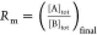. [B]_tot,final is different from [B]₀ because of the change in volume.

Table 1. Overview of Experiments Each Performed Six Times for the Reproducibility Test of ITC^a.

	titrant	[TOA] (M)	injections	Rm
A	pure HAc	0.48	2 × 3 μL, 5 × 5 μL, 15 × 10 μL, 13 × 15 μL	7.3
B	pure HAc	0.24	3 μL, 5 × 5 μL, 15 × 10 μL, 7 × 15 μL	7.5
C	50 vol % HAc in toluene	0.12	3 μL, 2 × 5 μL, 11 × 10 μL	9.5

^aAcetic acid (HAc) is titrated into TOA dissolved in toluene at 20 °C.

Theory

This section gives an overview of the methods and errors of ITC analysis that have been reported in the literature, presents the calculation method for the thermodynamic parameters, and discusses different reaction mechanisms and models of fitting.

Fitting of ITC data

The fitting models described in the literature on ITC data fitting include a 1:1 complexation,^36,38 a single set of identical sites yielding a similar fit to 1:1 complexation,^29,39 or sequential binding of the ligands to the complex.⁴⁰ Some authors used customized scripts,⁴¹ including also agglomeration of specific complexes or the effect of competing ligands. In this work only basic models based on a single set of identical sites (with the possibility to vary the stoichiometry) and on sequential binding will be compared for the fitting of acid–amine complexation in toluene.

The sequential reaction model starts with formation of 1:1 complexes according to eq 1, and the equilibrium constant of this complex formation K_1,1 is defined in eq 2.

1

2

From these two parameters, both ΔG and ΔS can be calculated using eqs 3 and 4.

3

4

For higher stoichiometries, extra equations can be added to the system of eqs 1 and 2. For a second molecule of A interacting with the complex AB to form the complex A₂B, the reaction equation and equilibrium constant are shown in eqs 5 and 6.

5

6

By fitting these equations to the heat release of the ITC experiment, not only ΔH_1,1 and K_1,1 can be obtained but also ΔH_2,1 and K_2,1. In the Supporting Information the theoretical ITC curves are displayed for a single reaction model with 1:1 stoichiometry (eqs 1 and 2) and for a reaction system based on two reaction equations (eqs 1, 2, 5, and 6). For a varying stoichiometry n in the second reaction the reaction mechanism can also consist of multiple equations; i.e., next to eq 2 the sequential series of equations defined by the constant in eq 7 are fitted, and at least a clear double S-curve is needed for a decent fit (see the Supporting Information, Figure S1b). For the fitting procedure, initial guess values were taken that are typical for hydrogen bonding and proton exchange (i.e., K_1,1 = 10, ΔH_1,1 = −30 kJ/mol, K_n+1,1 = 100, ΔH_n+1,1 = −18 kJ/mol, and n = 1.6). In this reaction n molecules of A interact with the AB complex.

7

Fitting ITC data to this kind of multiple-site model has been reported by Brautigam⁴³ (details in the Supporting Information), and similar to his findings, also for the acid extractions a model may be used based on two different types of interaction. In the case of inactive diluents, higher stoichiometry complexes are formed where only one acid interacts directly with the base,²⁸ and the subsequent acids add to the complex through hydrogen bonding. For this sequential binding, the interaction between the first acid with the base is different, but all other interactions are considered equal in energy, i.e., ΔH_1,1 and ΔH_n+1,1, respectively. The corresponding equilibrium constants and enthalpies of complexation are the fit parameters of this model next to the stoichiometry n.

Since models with multiple reactions require extensive fitting procedures and large sets of data, a simpler model could be advantageous. A potential model is a single reaction model based on a single set of identical sites. In this model an average stoichiometry is used for the fitting and it is assumed that the interaction of each compound is equal. The reaction equation is similar to the one in eq 1. However, for this system an average stoichiometry is used; see eq 8 with corresponding equilibrium constant in eq 9. In this model only one molecule of B reacts with n molecules of A. The stoichiometry coefficient n does not occur as an exponent of the concentration of A, because this would imply a sequential reaction mechanism.

8

9

Error in Parameters

Under ideal conditions the main source of error is the error in volume and this results in a statistical error of approximately 1% for ΔH and K. In actual experiments in an ITC machine, errors of around 1% for H and 5% for K were found.⁴² Based on a comparison of results from different laboratories, the calculated error in ITC experiments appeared to be even larger. Errors were reported⁴² in both ΔG and ΔH of 3–4 kJ/mol, and since ΔS is derived from these parameters the error is 6–8 kJ/mol in TΔS, where in this case typical values for ΔG are around −50 kJ/mol, for ΔH between +20 and −20 kJ/mol and TΔS around 50 kJ/mol.⁴² There are very large differences in the reported accuracy of the fitted parameters; e.g., very large errors for thiophenol were found as a result of very low heat of injection for specific compounds.²⁹ The error in ΔG is not mentioned very often, but it should be smaller than the error in ΔH because ΔG is logarithmically dependent on K; see eq 3.³⁶

For the models applied in this study, i.e., the single reaction model of eqs 8 and 9 and the sequential reaction model of eqs 1, 2, and 7, the total heat released after each injection Q_tot was calculated with eqs 10 and 11, respectively. In these equations V_tot is the total volume of sample and titrant present in the sample cell.

10

11

To compare the fitting statistics with the theoretical sensitivity of the fitted ΔH, K, and n for errors in experimental data under the conditions applied in this study, an analysis was performed making use of a Monte Carlo simulation. An ideal set of data points was generated based on fixed values for the parameters K, ΔH, and n, for the sequential reaction model, and a normally distributed random error with a standard deviation of 1% in the heat of injection was added as noise. From eqs 10 and 11 it can be concluded that a simulated random error in other variables such as the sample volume or injected volume will also directly result in an error in the heat of injection. Data sets were simulated based on the following assumptions: initial volume (V_init) is 2.72 mL, amount of extractant (n_base) is 6.6 × 10^–4 mol (corresponding to an initial concentration of 0.24 M), K_1,1 = 12, H_1,1 = −28 kJ/mol, K_n+1,1 = 118, ΔH_n+1,1 = −15 kJ/mol, and n = 1.6. These values are similar to parameters fitted on experimental data.

Results and Discussion

Two injection procedures for ITC experiments have been studied, i.e., through a series of periodical injections, including a study of the accuracy of the fitted parameters and the effect of measurement data on the fitted parameters, and through continuous injection, which may reduce analysis time.

Periodical Injection

In a typical ITC experiment with periodical injection, in which pure acetic acid was titrated to 0.24 M TOA in toluene mixture, the first six injection volumes were smaller (injection 1, 3 μL; injections 2–6, 5 μL) than the following injections (10–15 μL) to obtain a higher data density in these regions of the S-curve, which eases the fitting of the experimental data. The direct experimental results for this experiment are shown in Figure 1.

Figure 1.

Raw data for ITC analysis of titration of pure acetic acid into 0.24 M TOA in toluene at 20 °C.

In Figure 1, initially the signals with the same injection volume (injections 2–6) have comparable signals. The very first point shows a small signal, even if the smaller volume of 3 μL instead of 5 μL is taken into account. It is common that the first point is off, and this is due to loss of the titrant by diffusion.³⁶ The signal is positive, which means that the interaction is exothermic and up to 20 kJ/mol acid is released, which is a value that is in agreement with the literature on amine–carboxylic acid interactions.^27,34 Above a molar ratio of approximately 2 the intensity of the heat release reduces, until after a ratio of more than 5.5 only the enthalpy of mixing is measured.

Blank Measurements

Next to extractant–solute interactions, also the heat of interaction with the diluent might affect the results, and to investigate the thermal effects due to diluent interactions, blank measurements for titration of acetic acid into several diluents have been performed, shown in Figure 2. For some of the diluents, such as toluene, there is a strong change in the heat of injection in the first few injections. For other diluents, such as 1-octanol, the heat of injection is similar for all injections (excluding the first data point). The heat effects are a combination of the heat of dilution of the titrant and the heat of dilution of the diluent. If a diluent is very apolar and inactive, e.g., heptane or toluene, the (endothermic) heat effect of the first few injections of the highly polar and active acid can be very strong, which is primarily due to breaking of hydrogen bonds between the acid molecules that are diluted into an apolar environment. With addition of the acid, the environment becomes more polar and the heat effect of future additions decreases. For the active diluent 1-octanol the heat effect of most injections is similar, due to its hydrogen bonding ability, and upon injection of acid, there are no significant net hydrogen bonding effects. For all parameter fits, ITC raw data were corrected with the blank measurement data to correct for the heat effects due to diluent effects, assuming that the heat of dilution is equal for pure diluent and for the solvent mixtures used in the actual experiments.⁴²

Figure 2.

Blank experiments for titrating acetic acid into the pure diluent (no extractant) at 20 °C, for ◇, heptane; ▼, MIBK; ■, 1-octanol (50 vol % acid); ▲, toluene; and ●, 1-octanol (pure acid).

Diluent Effects

Before discussing quantitatively fitting results for one type of diluent, a set of experiments with different diluents is presented here and the shapes of the integrated and diluent effect corrected experimental ITC results are compared phenomenologically. Among the results in Figure 3a is the curve corresponding to the experiment with acetic acid and TOA in toluene that was shown in Figure 1, as well as an experiment with MIBK and one with heptane. For the diluent toluene, the heat released as a result of the first few injections is large compared to the following injection. The graph shows a double S-shape, also shown in Figure S1b, implying that the enthalpy of complexation of the first acid is larger negative than that of the second and following acids. For all three diluents the intensity of the heat release reduced after a stoichiometry of approximately 2. The MIBK graph shows a low energy release as a result of the first few injections, which then increases first before reducing again at stoichiometry of >2, indicating that here the presence of the first acid promotes the subsequent acid–complex binding. For heptane there is no remarkable high or low heat released for the first injections and the graph shows a plateau. Figure 3b shows the results when 1-octanol was applied as the diluent. In this case the energy released in the first injections is higher and the energy release already reduces at stoichiometry of >1. This indicates that interaction with the first acid is stronger and that the (1,1) complex is the main complex formed. This is a result of competition between 1-octanol and acetic acid for binding with the extractant molecule.²⁸

Figure 3.

Differences in shape of isotherm (S-curve) for titration of pure acetic acid to 0.24 M TOA at 20 °C in (a) ■, toluene; △, MIBK; and ○, heptane; and (b) ●, 1-octanol.

To compare the two types of models, it was attempted to fit the characteristic result obtained with toluene both with the single reaction model using an average stoichiometry (eqs 8 and 9), and with the sequential reaction model (eqs 1, 2, and 7). The best-fit isotherms are shown in Figure 4. For the major part of the curves, both models fit (almost) similarly and the residuals of the fits are 3.2% for the sequential model and 4.8% for the single reaction model. However, especially at the first part of the curves, the sequential reaction model gives a much better fit for the experimental data; see Figure 4. The lower heat release in the first injections for MIBK may be a result of a similar enthalpy of complexation for the first and following acids and a lower complexation constant of the first complex in MIBK; see Table S1 in the Supporting Information for details on the fitted parameters. For heptane, the plateau indicates similar enthalpies of complexation for the acids interacting with the amine in combination with a moderate K_1,1. Because of the plateau, the single reaction model is a better fit for heptane compared to toluene and MIBK.

Figure 4.

Fit of experimental data obtained with titration of acetic acid to 0.24 M TOA in toluene at 20 °C. The model lines represent the sequential reaction model (dotted line) and the single reaction model (dashed–dotted line) described in eqs 1, 2, and 7 and in eqs 8 and 9, respectively. Fitted parameters are shown in Table S1 in the Supporting Information.

Without going further in depth on why these diluents induce these differences, it is clear that these differences are important for the proper fitting of the thermodynamic parameters to the experimental data. For a proper fit with the model based on a single set of identical sites, either very similar values for the complexation enthalpy of the different acids are required, or a 1:1 stoichiometry of the complexation is required. When larger complexes are formed with different enthalpies of complexation of the acids, the sequential binding model is more applicable.

Accuracy of Fitted Parameters from ITC Experiments

To investigate the accuracy and reproducibility of ITC experiments and study the effect of the concentration of the titrant and the concentration of extractant in the sample mixture, the experiments from Table 1 were each performed six times. For each of the experiments, the parameters were fitted to the experimental data, and then the average values of the fitted constants and their corresponding standard deviation were calculated. Because the K-values are dependent on n (eq 9), they cannot be directly compared with each other and the resulting averages should only be used for determining the sensitivity of the parameter to experimental errors. The fitted parameter values as well as the fitting statistics for the single reaction model are given in Table 2, and in Table 3 the results for the sequential reaction model with the same experimental data are given. For both models, the stoichiometry of the amine is assumed to be m = 1, because overloading of a single amine is expected.^27,28 A very important observation from Tables 2 and 3 is that the values of the equilibrium constants are dependent on the concentration of amine. This is a logical result, since the amine affects the properties of the solution (e.g., polarity, availability of hydrogen bond donating and accepting groups), and it shows that it is very important to study interactions at the same concentration as will be used in a practical application such as LLX. The standard deviations of K_n,1 and ΔH_n,1 are lower using the third experimental method with a lower concentration of 0.12 M TOA, which is most likely a result of the lower concentration of acid in the titrant allowing for a larger number of injections and larger injection volumes per mole of titrant and therefore less error in injection volume. For fitting of the stoichiometry n the first method with 0.24 M TOA shows a slightly lower standard deviation; however, the relative standard deviations in ΔH_n,1 and n are for all three methods less than 3.5%. With the relative standard deviation up to 13%, the accuracy in K_n,1 is lower.

Table 2. Calculated Values for K_n,1, n, ΔH_n,1, and Fit Residue for Fitting of the Experimental Data for Three Experimental Data Sets (See Table 1) Fitted with the Single Reaction Model of Eqs 8–10.

data set		Kn,1	n	ΔHn,1 (kJ/mol)	fit residue (%)
pure HAc to 0.48 M TOA in toluene	average	23.6	2.96	–19.8	4.3
	std dev	3.11	0.10	0.65	1.3
	rel std dev (%)	13	3.5	3.3
pure HAc to 0.24 M TOA in toluene	average	35.6	2.8	–20.8	4.3
	std dev	4.39	0.045	0.52	1.1
	rel std dev (%)	12	1.6	2.5
50 vol % HAc to 0.12 M TOA in toluene	average	38.8	2.79	–22.7	4.4
	std dev	0.50	0.09	0.17	0.4
	rel std dev (%)	1.29	3.34	0.76

Table 3. Calculated Values for K_1,1, ΔH_1,1, K_n+1,1, ΔH_n+1,1, n, and Fit Residue for Fitting of the Experimental Data for Three Experimental Data Sets (See Table 1) Fitted with the Sequential Reaction Model of Eqs 1, 2, 7, and 11.

data set		K1,1	ΔH1,1 (kJ/mol)	Kn+1,1	ΔHn+1,1 (kJ/mol)	n	fit residue (%)
pure HAc to 0.48 M TOA in toluene	average	16.7	–25.3	53.8	–18.3	1.73	5.6
	std dev	6.14	1.26	15.4	0.93	0.08	1.5
	rel std dev (%)	37	5.0	29	5.1	4.7
pure HAc to 0.24 M TOA in toluene	average	12.7	–30.0	97.0	–15.6	1.58	3.6
	std dev	1.46	1.25	25.2	1.95	0.02	0.9
	rel std dev (%)	11	4.2	26	12	1.4
50 vol % HAc to 0.12 M TOA in toluene	average	18.5	–34.6	168	–14.9	1.59	4.1
	std dev	1.10	0.94	38.0	1.83	0.03	1.3
	rel std dev (%)	6.0	2.7	23	12	1.9

Also, K_1,1 shows a very high standard deviation of 37% when 0.48 M TOA is used, compared to 11% for the method with 0.24 M TOA and 6.0% for the method with 0.12 M TOA. Apparently fitting of the first K-value is more difficult at the higher concentration of TOA or the lower number of injections, which can also be seen in very low (relative) standard deviations in both fitted K-values (6.0% in K_1,1 and 23% in K_n+1,1) in the case of 0.12 M TOA. Next to the effect of more injections or a larger injection volume with 50% acetic acid, at a lower concentration of TOA the maximum slope of the titration curve is less steep, allowing more data points in the steep part of the curve, which may decrease the error in the obtained K-parameters. For the other two methods the relative standard deviations in K_n+1,1 are also large, with 26% for 0.24 M TOA and 29% for 0.48 M TOA. Similar to the results in Table 2, the relative standard deviations in the fitted values of n and ΔH_1,1 are very low, especially in the cases of 0.12 M TOA (1.9% in n and 2.7% in ΔH_1,1) and 0.24 M TOA (1.4% in n and 4.2% in ΔH_1,1), and with 0.48 M TOA at 4.7% in n and 5.0% in ΔH_1,1 still acceptable.

When the results of the single reaction model are compared with those of the sequential reaction model, it can be seen that overall the residues of fit of both models are comparable and have reasonable values, <10%. However, it should be mentioned that, as shown in Figure 4, the much better fit of the sequential reaction model in the first part of the curve does not strongly affect the overall residue of fit. Nevertheless, to properly describe this phenomenological effect, the sequential reaction model is much better suited. For the second method with 0.48 M TOA, the residue of fit and the standard deviation of the K-values are larger for the sequential reaction model; this increased fitting error is probably due to the lower n_inj that was applied in this method. For one of the experiments with 0.24 M TOA, the 95% confidence intervals of the parameter fit were also determined. For ΔH_1,1 (=28.8 kJ/mol) the interval ranged from −33.7 to −24.0 kJ/mol; for K_1,1 (=11.7) the interval was only very small and ranged from 11.70 to 11.71. For the parameters of the second reaction the intervals were larger: for ΔH_n+1,1 (= –16.8 kJ/mol) the interval ranged from −21.0 to −12.6 kJ/mol, for K_n+1,1 (=96.7) the interval ranged from 76.4 to 117, and for n (=1.55) the interval ranged from 1.45 to 1.64.

When the three experimental methods are compared for the sequential binding model based on their c-values and number of injections n_inj (see Table 4), it can be seen that all the c-values are in the “ideal” range between 10 and 100. Comparing the methods and assuming that increasing the TOA concentration does not strongly increase the measurement accuracy, there is no clear advantage of the increased n_inj or c-value for fitting of the single reaction model. However, for the sequential reaction model the fit residues are smaller when a higher number of injections was applied in the analysis. The increased number of injections increases the data density, thereby enabling a better parameter fit.

Table 4. c-Values and Number of Injections for the Three Experimental Data Sets Applied.

					fit residue (%)
	titrant	[TOA] (M)	c-value	ninj	single reaction	sequential reaction
A	pure HAc	0.48	34	14	4.3	5.6
B	pure HAc	0.24	24	28	4.3	3.6
C	50 vol % HAc in toluene	0.12	13	34	4.4	4.1

Comparing the Errors Based on Experimental Data Fitting with Theoretical Errors Based on Simulation

To determine the theoretical effect of errors in the measurement data on the fitting of the parameters, Monte Carlo simulations were run with series of simulated data. Over sequential reaction model simulations a noise was added with a standard deviation (σ) of 1%, and these data were used to fit the model parameters; see Table 5 (top row). Detailed and additional results for lower concentration of extractant are shown in the Supporting Information. The K-values are more sensitive to errors in the experimental data than the other parameters. However, comparing with the original values for the parameters, it appears that a local minimum is reached. The possibility of a local minimum for the parameter fit was also suggested by Brautigam⁴³ and Le et al.,⁴⁴ which means that the fit depends on the initial values (K_1,1 = 10, H_1,1= −30 kJ/mol, K_n+1,1 = 80, ΔH_n+1,1= −12 kJ/mol, and n = 1.8). Because of this local minimum the data were fitted again by using the original values for the parameters as initial values; see Table 5 (fourth row). This does result in average values of the parameters that are around the original values, and smaller standard deviations in the fitted parameters of 0.5–2%. The single reaction model results are presented in the Supporting Information, and do not show dependency on initial estimates. Comparing the theoretical fit accuracy based on the Monte Carlo simulation on simulated data (Table 5) with the fit on experimental data (Table 3) shows that the fitting on experimental data results in significantly less accurate parameter fits. This indicates that either the error in the heat measured is significantly larger, also possibly not normally distributed, or other errors (e.g., volume, concentration) play a significant role.

Table 5. Parameter Fit for K_1,1, ΔH_1,1, K_n+1,1, ΔH_n+1,1, n, and Fit Residue for Fitting 170 Series of Simulated Data with the Sequential Reaction Model of Eqs 1, 2, and 7 for a 0.24 M TOA System.

data set		K1,1	ΔH1,1 (kJ/mol)	Kn+1,1	ΔHn+1,1 (kJ/mol)	n	fit residue (%)
simulated data set, σ = 0.01	average	7.92	–32.6	162	–11.4	1.65	2.8
	std dev	0.44	0.72	22	0.56	0.05	2.0
	rel std dev (%)	5.6	2.2	14	4.9	3.0
simulated data set, σ = 0.01a	average	12.0	–28.0	118	–15.0	1.60	0.9
	std dev	0.12	0.142	2.5	0.13	0.0099	0.2
	rel std dev (%)	0.99	0.51	2.1	0.87	0.62

^aOriginal values used as initial values.

To study the dependency of the fitted parameters on each other, the value for n was fixed and only the other two parameters were fitted. The initial values applied were the same as those mentioned above for the results in the top row of Table 5. Although the residue of the fit increased from 2.8 (top row of Table 5) to 3.2%, the only parameter that changed significantly in average value and confidence interval was K_n+1,1. The value decreased to 121 with a new 95% confidence interval from 115 to 128. Apparently only K_n+1,1 is dependent on n and these parameters are able to (partially) compensate each other in the fitting.

Continuous Injection

Next to injecting periodically, continuous injection of the titrant into the sample cell is also possible.⁴⁵ A comparison between periodical injection and continuous injection is shown in Figure 5. It can be seen that the experiment with heat-flow correction results in large noise on the curve. When dynamic correction was applied in the ITC experiment, the noise was significantly reduced. The problem with continuous injection appears to be the delay in the signal. For the faster injection (0.27 μmol/s, Figure 5, dotted line) the curve is moved to the right compared to the periodical injection where there is enough time to reach equilibrium at each point. For the slower injection (0.12 μmol/s (Figure 5, dashed line)), this effect is only seen in the first part of the curve (where the heat of injection has a larger negative value). Decreasing the rate of injection even further would lead to better results, but this also increases the experiment time to a longer time than when periodical injections are applied, thereby making the application of continuous injection less advantageous.

Figure 5.

ITC curve comparing method of continuous injection (lines) with periodical injection (titration) (■). Titration of acetic acid to 0.24 M TOA in water-saturated 1-octanol at 20 °C. Continuous injection was performed using dynamic correction at 0.12 μmol/s (dashed line) and 0.27 μmol/s (dotted line) and using heat flow correction at 0.27 μmol/s (continuous gray line).

Comparison with Reported ITC Accuracy in Literature

In this work the accuracy of the fitted parameters for the acid–base interactions in the concentration range applicable to liquid–liquid extraction was determined. To put these results into perspective, Table S5 in the Supporting Information shows experimental specifications and a summary of the accuracy reported in this work in combination with results published for other applications. Although the concentrations applied in this work are higher, the standard deviations obtained in the parameters for the single reaction model are comparable to those reported in other sources for one set of site models and 1:1 reaction models.^{29,36,38,39,46} No other source reported on the exact same sequential model. Brautigam,⁴³ however, reported a noise level of about 1% for two- and three-site models, which is more accurate compared to the standard deviation for ΔH_1,1 in this work. Also, for a three-site model Freyer et al.⁴⁰ reported an error of 0.5–6% for ΔH which is similar to the standard deviation in this work and they reported an error of 7–10% for K, which is more accurate.

Conclusion

The use of ITC to analyze interactions in high concentration domains was studied for acid–base interactions relevant for liquid–liquid extraction. The parameter estimation accuracy was evaluated for acetic acid complexation with TOA in toluene. Because it was found that the complexation constants are extractant concentration dependent, it is key that ITC analysis is performed at the concentration also applied in the liquid–liquid extraction process. Furthermore, based on a phenomenological study, it was concluded that a sequential reaction model is more suitable to fit ITC results for acid–base titration than a single reaction model. For the sequential reaction model, the parameters ΔH, K, and n were fitted on experimental periodical injection data with standard deviations of respectively 2.7–12, 6.0–37, and 1.4–4.7%. Fitting of such multiparameter models was found to be sensitive to local minima, indicating the importance of good initial guess values. In order to benchmark the accuracy of the parameter fit on experimental data, also theoretical parameter fits were done for Monte Carlo simulated data with a 1% noise in the data. From these results, it was found that the error in the parameters fitted on real experimental data is larger than the theoretical 0.5–2.1%, but still allows for accurate parameter estimation. The accuracy of the parameters fitted is the highest when a periodical injection is applied in combination with a lower concentration of TOA and a higher number of injections. Continuous injection posed no improvement compared to periodical injection due to a delay in the obtained power signal that requires a low rate of injection of titrant and therefore longer measurement time than the periodical injection, instead of the shorter time anticipated.

Supporting Information Available

The Supporting Information is available free of charge on the ACS Publications website at DOI: 10.1021/acs.iecr.8b03066.

• Experimental methods to minimize the error in ITC; more extensive discussion on theoretical ITC curves that supports the ITC curve-fitting discussion in the main article (PDF)

The authors declare no competing financial interest.

References

- Kabiri M.; Unsworth L. D. Application of Isothermal Titration Calorimetry for Characterizing Thermodynamic Parameters of Biomolecular Interactions: Peptide Self-Assembly and Protein Adsorption Case Studies. Biomacromolecules 2014, 15, 3463–3473. 10.1021/bm5004515. [DOI] [PubMed] [Google Scholar]
- Falconer R. J. Applications of isothermal titration calorimetry - the research and technical developments from 2011 to 2015. J. Mol. Recognit. 2016, 29, 504–515. 10.1002/jmr.2550. [DOI] [PubMed] [Google Scholar]
- Tsvetkov P. O.; Barbier P.; Breuzard G.; Peyrot V.; Devred F. Microtubule-associated proteins and tubulin interaction by isothermal titration calorimetry. Methods Cell Biol. 2013, 115, 283–302. 10.1016/B978-0-12-407757-7.00018-9. [DOI] [PubMed] [Google Scholar]
- Damian L. Isothermal titration calorimetry for studying protein-ligand interactions. Methods Mol. Biol. (N. Y., NY, U. S.) 2013, 1008, 103–118. 10.1007/978-1-62703-398-5_4. [DOI] [PubMed] [Google Scholar]
- Demarse N. A.; Killian M. C.; Hansen L. D.; Quinn C. F. Determining enzyme kinetics via isothermal titration calorimetry. Methods Mol. Biol. (N. Y., NY, U. S.) 2013, 978, 21–30. 10.1007/978-1-62703-293-3_2. [DOI] [PubMed] [Google Scholar]
- Aweda T. A.; Meares C. F. Combination of isothermal titration calorimetry and time-resolved luminescence for high affinity antibody-ligand interaction thermodynamics and kinetics. Methods (Amsterdam, Neth.) 2012, 56, 145–153. 10.1016/j.ymeth.2011.09.011. [DOI] [PMC free article] [PubMed] [Google Scholar]
- Roselin L. S.; Lin M.-S.; Lin P.-H.; Chang Y.; Chen W.-Y. Recent trends and some applications of isothermal titration calorimetry in biotechnology. Biotechnol. J. 2010, 5, 85–98. 10.1002/biot.200900092. [DOI] [PubMed] [Google Scholar]
- Wilcox D. E. Isothermal titration calorimetry of metal ions binding to proteins: An overview of recent studies. Inorg. Chim. Acta 2008, 361, 857–867. 10.1016/j.ica.2007.10.032. [DOI] [Google Scholar]
- Ladbury J. E.; Chowdhry B. Z. Sensing the heat: the application of isothermal titration calorimetry to thermodynamic studies of biomolecular interactions. Chem. Biol. 1996, 3, 791–801. 10.1016/S1074-5521(96)90063-0. [DOI] [PubMed] [Google Scholar]
- Liang Y. Applications of isothermal titration calorimetry in protein science. Acta Biochim. Biophys. Sin. 2008, 40, 565–576. 10.1111/j.1745-7270.2008.00437.x. [DOI] [PubMed] [Google Scholar]
- Huang R.; Lau B. L. T. Biomolecule–nanoparticle interactions: Elucidation of the thermodynamics by isothermal titration calorimetry. Biochim. Biophys. Acta, Gen. Subj. 2016, 1860, 945–956. 10.1016/j.bbagen.2016.01.027. [DOI] [PubMed] [Google Scholar]
- Omanovic-Miklicanin E.; Manfield I.; Wilkins T. Application of isothermal titration calorimetry in evaluation of protein–nanoparticle interactions. J. Therm. Anal. Calorim. 2017, 127, 605–613. 10.1007/s10973-016-5764-4. [DOI] [Google Scholar]
- Fox J. M.; Kang K.; Sherman W.; Héroux A.; Sastry G. M.; Baghbanzadeh M.; Lockett M. R.; Whitesides G. M. Interactions between Hofmeister Anions and the Binding Pocket of a Protein. J. Am. Chem. Soc. 2015, 137, 3859–3866. 10.1021/jacs.5b00187. [DOI] [PMC free article] [PubMed] [Google Scholar]
- Bharmoria P.; Kumar A. Thermodynamic investigations of protein’s behaviour with ionic liquids in aqueous medium studied by isothermal titration calorimetry. Biochim. Biophys. Acta, Gen. Subj. 2016, 1860, 1017–1025. 10.1016/j.bbagen.2015.08.022. [DOI] [PubMed] [Google Scholar]
- Beezer A. E.; Hawksworth W. A.; Orban M.; Tyrrell H. J. V. Hydrogen-bonded complexes between pyridine and phenol in carbon tetrachloride solutions. J. Chem. Soc., Faraday Trans. 1 1977, 73, 1326–1333. 10.1039/f19777301326. [DOI] [Google Scholar]
- Barton S. S.; Kraft J. P.; Owens T. R.; Skinner L. J. A calorimetric study of phenol-pyridine complexes in carbon tetrachloride solution. J. Chem. Soc., Perkin Trans. 2 1972, 2, 339–341. 10.1039/P29720000339. [DOI] [Google Scholar]
- Zaretskii M. I. Complexation of the pyridine bases in the products from the coking of coal with organic solvents (review). Chem. Heterocycl. Compd. 1997, 33, 1–16. 10.1007/BF02290741. [DOI] [Google Scholar]
- Arnett E. M.; Joris L.; Mitchell E.; Murty T. S. S. R.; Gorrie T. M.; Schleyer P. v. R. Hydrogen-bonded complex formation. III. Thermodynamics of complexing by infrared spectroscopy and calorimetry. J. Am. Chem. Soc. 1970, 92, 2365–2377. 10.1021/ja00711a029. [DOI] [Google Scholar]
- Freire E.; Mayorga O. L.; Straume M. Isothermal titration calorimetry. Anal. Chem. 1990, 62, 950A–959A. 10.1021/ac00217a002. [DOI] [Google Scholar]
- Ghai R.; Falconer R. J.; Collins B. M. Applications of isothermal titration calorimetry in pure and applied research—survey of the literature from 2010. J. Mol. Recognit. 2012, 25, 32–52. 10.1002/jmr.1167. [DOI] [PubMed] [Google Scholar]
- Loh W.; Brinatti C.; Tam K. C. Use of isothermal titration calorimetry to study surfactant aggregation in colloidal systems. Biochim. Biophys. Acta, Gen. Subj. 2016, 1860, 999–1016. 10.1016/j.bbagen.2015.10.003. [DOI] [PubMed] [Google Scholar]
- Boudker O.; Oh S. Isothermal titration calorimetry of ion-coupled membrane transporters. Methods 2015, 76, 171–182. 10.1016/j.ymeth.2015.01.012. [DOI] [PMC free article] [PubMed] [Google Scholar]
- Draczkowski P.; Matosiuk D.; Jozwiak K. Isothermal titration calorimetry in membrane protein research. J. Pharm. Biomed. Anal. 2014, 87, 313–325. 10.1016/j.jpba.2013.09.003. [DOI] [PubMed] [Google Scholar]
- Traut T.Allosteric Regulatory Enzymes; Springer: New York, 2008. [Google Scholar]
- Freiburger L. A.; Baettig O. M.; Sprules T.; Berghuis A. M.; Auclair K.; Mittermaier A. K. Competing allosteric mechanisms modulate substrate binding in a dimeric enzyme. Nat. Struct. Mol. Biol. 2011, 18, 288–294. 10.1038/nsmb.1978. [DOI] [PMC free article] [PubMed] [Google Scholar]
- Freiburger L.; Auclair K.; Mittermaier A. Global ITC fitting methods in studies of protein allostery. Methods 2015, 76, 149–161. 10.1016/j.ymeth.2014.12.018. [DOI] [PMC free article] [PubMed] [Google Scholar]
- Tamada J. A.; Kertes A. S.; King C. J. Extraction of carboxylic acids with amine extractants. 1. Equilibria and law of mass action modeling. Ind. Eng. Chem. Res. 1990, 29, 1319–1326. 10.1021/ie00103a035. [DOI] [Google Scholar]
- Tamada J. A.; King C. J. Extraction of carboxylic acids with amine extractants. 2. Chemical interactions and interpretation of data. Ind. Eng. Chem. Res. 1990, 29, 1327–1333. 10.1021/ie00103a036. [DOI] [Google Scholar]
- Cuypers R.; Burghoff B.; Marcelis A. T. M.; Sudhölter E. J. R.; de Haan A. B.; Zuilhof H. Complexation of Phenols and Thiophenol by Phosphine Oxides and Phosphates. Extraction, Isothermal Titration Calorimetry, and ab Initio Calculations. J. Phys. Chem. A 2008, 112, 11714–11723. 10.1021/jp801605y. [DOI] [PubMed] [Google Scholar]
- Cuypers R.; Murali S.; Marcelis A. T. M.; Sudhoelter E. J. R.; Zuilhof H. Complexation of Phenol and Thiophenol by Amine N-Oxides: Isothermal Titration Calorimetry and ab Initio Calculations. ChemPhysChem 2010, 11, 3465–3473. 10.1002/cphc.201000482. [DOI] [PubMed] [Google Scholar]
- Ziegenfuβ H.; Maurer G. Distribution of acetic acid between water and organic solutions of tri-n-octylamine. Fluid Phase Equilib. 1994, 102, 211–255. 10.1016/0378-3812(94)87078-0. [DOI] [Google Scholar]
- Ingale M. N.; Mahajani V. V. Recovery of acetic acid and propionic acid from aqueous waste stream. Sep. Technol. 1994, 4, 123–126. 10.1016/0956-9618(94)80014-6. [DOI] [Google Scholar]
- Scheler C.; Popovic M.; Iannotti E.; Mueller R.; Bajpai R. Chemical interactions between aqueous and organic phases in a reactive extraction process. Appl. Biochem. Biotechnol. 1996, 57, 29. 10.1007/BF02941685. [DOI] [Google Scholar]
- Marti M. E. Solvent modification effect on the physical and chemical extraction of acetic acid. Sep. Sci. Technol. 2016, 51, 1806. 10.1080/01496395.2016.1178286. [DOI] [Google Scholar]
- Rasrendra C. B.; Girisuta B.; van de Bovenkamp H. H.; Winkelman J. G. M.; Leijenhorst E. J.; Venderbosch R. H.; Windt M.; Meier D.; Heeres H. J. Recovery of acetic acid from an aqueous pyrolysis oil phase by reactive extraction using tri-n-octylamine. Chem. Eng. J. 2011, 176–177, 244–252. 10.1016/j.cej.2011.08.082. [DOI] [Google Scholar]
- Boyce S. E.; Tellinghuisen J.; Chodera J. D.. Avoiding accuracy-limiting pitfalls in the study of protein-ligand interactions with isothermal titration calorimetry. 2015. bioRxiv 023796. 10.1101/023796. [DOI]
- Wiseman T.; Williston S.; Brandts J. F.; Lin L.-N. Rapid measurement of binding constants and heats of binding using a new titration calorimeter. Anal. Biochem. 1989, 179, 131–137. 10.1016/0003-2697(89)90213-3. [DOI] [PubMed] [Google Scholar]
- Tellinghuisen J. Statistical error in isothermal titration calorimetry: Variance function estimation from generalized least squares. Anal. Biochem. 2005, 343, 106–115. 10.1016/j.ab.2005.04.026. [DOI] [PubMed] [Google Scholar]
- Liu Y.; Sturtevant J. M. Significant discrepancies between van’t Hoff and calorimetric enthalpies. Biophys. Chem. 1997, 64, 121–126. 10.1016/S0301-4622(96)02229-6. [DOI] [PubMed] [Google Scholar]
- Freyer M. W.; Lewis E. A.. Methods in Cell Biology; Academic Press: 2008; pp 79–113. [DOI] [PubMed] [Google Scholar]
- Tellinghuisen J. Designing isothermal titration calorimetry experiments for the study of 1:1 binding: problems with the ″standard protocol″. Anal. Biochem. 2012, 424, 211–220. 10.1016/j.ab.2011.12.035. [DOI] [PubMed] [Google Scholar]
- Schalley C. A.Analytical Methods in Supramolecular Chemistry; Wiley: Weinheim, Germany, 2007. [Google Scholar]
- Brautigam C. A. Fitting two- and three-site binding models to isothermal titration calorimetric data. Methods 2015, 76, 124–136. 10.1016/j.ymeth.2014.11.018. [DOI] [PMC free article] [PubMed] [Google Scholar]
- Le V. H.; Buscaglia R.; Chaires J. B.; Lewis E. A. Modeling complex equilibria in isothermal titration calorimetry experiments: Thermodynamic parameters estimation for a three-binding-site model. Anal. Biochem. 2013, 434, 233–241. 10.1016/j.ab.2012.11.030. [DOI] [PMC free article] [PubMed] [Google Scholar]
- Markova N.; Hallén D. The development of a continuous isothermal titration calorimetric method for equilibrium studies. Anal. Biochem. 2004, 331, 77–88. 10.1016/S0003-2697(04)00254-4. [DOI] [PubMed] [Google Scholar]
- Saha S.; Roy A.; Roy K.; Roy M. N. Study to explore the mechanism to form inclusion complexes of β-cyclodextrin with vitamin molecules. Sci. Rep. 2016, 6, 35764. 10.1038/srep35764. [DOI] [PMC free article] [PubMed] [Google Scholar]
Associated Data
This section collects any data citations, data availability statements, or supplementary materials included in this article.