Two-phase differential expression analysis for single cell RNA-seq

Abstract

Motivation

Single-cell RNA-sequencing (scRNA-seq) has brought the study of the transcriptome to higher resolution and makes it possible for scientists to provide answers with more clarity to the question of ‘differential expression’. However, most computational methods still stick with the old mentality of viewing differential expression as a simple ‘up or down’ phenomenon. We advocate that we should fully embrace the features of single cell data, which allows us to observe binary (from Off to On) as well as continuous (the amount of expression) regulations.

Results

We develop a method, termed SC2P, that first identifies the phase of expression a gene is in, by taking into account of both cell- and gene-specific contexts, in a model-based and data-driven fashion. We then identify two forms of transcription regulation: phase transition, and magnitude tuning. We demonstrate that compared with existing methods, SC2P provides substantial improvement in sensitivity without sacrificing the control of false discovery, as well as better robustness. Furthermore, the analysis provides better interpretation of the nature of regulation types in different genes.

Availability and implementation

SC2P is implemented as an open source R package publicly available at https://github.com/haowulab/SC2P.

Supplementary information

Supplementary data are available at Bioinformatics online.

1 Introduction

Studies of transcriptome have been arguably the most active field in genomics research. Traditionally, gene expression is measured from ‘bulk’ samples pooling a large number (often in the scale of millions) of cells, thus the measurements reflect the average expression of a population of cells. For highly heterogeneous samples such as cancer or brain tissues, the bulk measurements fail to provide more detailed information for the transcriptomic variation. For example, bulk expression data cannot differentiate a ‘50% decrease in all cells’ and a mixture of ‘complete shut-down in half of the cells, while no change in the other half’.

Single-cell RNA-sequencing (scRNA-seq) emerged recently as a powerful technology to investigate transcriptomic variation and regulation at the individual cell level (Buettner et al., 2015; Patel et al., 2014; Picelli et al., 2013; Ramsköld et al., 2012; Shalek et al., 2014; Tang et al., 2009; Usoskin et al., 2015). It is in scRNA-seq that we finally observe evidence of binary status of transcription (Shalek et al., 2013; Wills et al., 2013), which we refer to as ‘phases’ in transcription. Phase I corresponds to low level non-specific transcription (for example, as a result of random initiation), and Phase II corresponds to targeted specific transcription. The regulation of transcription includes a phase transition between Phase I and Phase II, as well as continuous regulation within Phase II.

Even though the analysis of scRNA-seq data is multifaceted, including cell clustering (Kiselev et al., 2017; Ntranos et al., 2016), pseudo-time construction (Trapnell et al., 2014) and rare cell type identification (Grün et al., 2015; Jiang et al., 2016), differential expression (DE) remains the most fundamental question to be answered. The scRNA-seq technology makes it possible for scientists to provide answers with more clarity even to the simple question of DE. Due to the special characteristics of scRNA-seq data, including excessive zero counts for both biological and technical reasons, higher variability and multi-modal distribution that cannot be attributed to the zero counts (Bacher and Kendziorski, 2016), DE methods developed for bulk RNA-seq cannot be directly applied. We illustrate some of these characteristics in Figure 1, where histograms of the log counts in three cells are presented. A spike of zero counts is observed in all three cells, most obvious in Cell A and to a less extent in Cells B and C. A substantial fraction of genes have non-zero but very low counts (with log2 counts less than 3). Another group of genes reach counts that are orders-of-magnitudes higher, sometimes forming a second mode, which is most obvious in Cell B. Cell B appears to have a greater proportion of genes with high expression level, though it also has more than twice as many genes with zero counts as seen in Cell C. These examples suggest that non-zero count is not a reliable reflection of expression activity and to dichotomize genes into on/off categories by one arbitrary cutoff may lead to systematic biases between cells.

Fig. 1.

Histogram of three cells in the human brain dataset. The y axis is trimmed at 500 to allow the visualization of lower frequencies. The parameters are described in the Methods section. π is the estimated prior proportion of genes in Phase II. (A) A cell with extremely high zero inflation, and a small fraction (8%) of genes in Phase II expression. (B) A cell with high zero inflation, but also a high proportion (32%) of genes in Phase II expression. (C) A cell with low zero inflation, but also small fraction (9%) in Phase II expression

Recently, a few methods were developed specifically for scRNA-seq DE. SCDE (Kharchenko et al., 2014) uses a mixture of Poisson and negative binomial distributions to capture the two phases, and then identifies DE when the gene is on. Monocle (Trapnell et al., 2014) uses a generalized additive model (GAM) to test the differences in marginal mean expressions; BPSC (Vu et al., 2016) uses a beta-Poisson mixture model to capture the bimodality in the expression, and then implements a generalized linear model (GLM) for DE test for, again, the differences in marginal mean expressions. Even though these methods have noticed and mentioned the phenomenon of two-phase transcription from scRNA-seq data, they dismissed the importance of the phase transition. Genes in Phase I are often considered technical ‘dropouts’ that failed to be detected, and the DE analyses are mostly focused on the marginal changes or within the Phase II, e.g. when the gene is ‘on’. Even when phase transition is considered in some methods, it is not recognized as an important form of DE in its own right. For example, MAST (Finak et al., 2015) includes a test for phase change but only declares a gene DE if ‘the estimated fold-change is greater than 1.5’ in addition to low FDR. $D^{3}E$ (Delmans and Hemberg, 2016) is a method based on a bursting model that explicitly considers ‘On’ and ‘Off’ status of gene expression. The detection of DE, however, is marginal: the method uses non-parametric or likelihood ratio tests to test a null hypothesis that the distributions of expression across two groups are identical. When the null is rejected, it does not infer the reason being a change in bursting rate or in burst size. Korthauer et al. (2016) also considers the possibility of multi-modal distribution of a gene’s expression, and presents a Bayesian modeling framework (scDD) that identifies differential distribution (DD) across conditions. The transition between phases is not directly inferred. Instead, genes that are identified as showing DD are subsequently classified by their patterns of difference, including mean shift, differential proportion of the same components, differential modality or a combinations of these.

We advocate that the lower mode in the distribution of gene expression corresponds to a phase of inactivity, and phase transition is the first important step in transcription regulation, hence it is essential to the understanding of the regulation mechanism. Thus a principled, data-driven approach rather than arbitrary cutoff for determining phase is necessary. We observe, in multiple biological systems, that DE can take the form of phase transition or magnitude tuning, and a combination of these two. Most interestingly, we observe examples of ‘compensation’ (presented in the Results section): a population of cells may have a lower percentage expressing a particular gene, but the cells expressing that gene do so at a higher level. In such cases, the average expression level may remain the same and be completely unidentifiable in bulk RNA-seq.

In this work, we present a statistical method, termed SC2P, that identifies the phase for each gene in each cell, given the context (both biological and technical) of each cell sample and gene-specific profile. With this latent phase inferred, we identify genes that go through different forms of DE. This includes genes that are turned on with different frequencies in different populations (Form I), as well as genes that are transcribed at different rates (Form II). These different forms of DE reveal, potentially, different mechanisms in the regulation of transcription, such as initiation versus elongation speed (Jonkers and Lis, 2015), bursting frequency versus bursting size (Dar et al., 2012; Raj et al., 2006), or different half-life of RNA transcripts. Being able to distinguish the forms of DE between cell types, or over time, will also elucidate the relationship between expression and genomic/epigenomic elements: some markers may be associated with the probability of expression while others may be associated with the amount of expression.

2 Materials and methods

2.1 Data model

We begin with the expression measured as sequence read counts for G genes and C cells in a G × C matrix Y. For a particular gene, we use a two-component mixture model to describe its expression from individual cells. This characterizes the phenomenon observed in multiple publicly available datasets (Darmanis et al., 2015; Shekhar et al., 2016) as well as our data that many genes demonstrate a bimodal distribution: one component corresponds to very low counts with an excess of zero, consistent with a background, inactive transcription; the other component corresponds to higher counts with a long right tail that are approximately normal in log scale. We refer to these as the two ‘phases’ of transcription. A key difference separating our model from those described in existing methods is our treatment of the first component, by allowing cell-specific parameters. The status of each gene in each cell, i.e. which component the observed count is generated from, is latent, but inferable given the observed count and the gene-cell contexts.

We use a zero-inflated Poisson (ZIP) distribution to model Phase I (inactive transcription), and a lognormal-Poisson (LNP) model for Phase II (targeted specific transcription). Specifically, let Y_gi denote the count observed on gene g in cell i, and Z_gi denote the binary latent expression state (Z_gi = 1 for Phase II). We model Phase I with a ZIP distribution $Y_{gi}|Z_{gi}=0\sim ZIP(p_i,{\lambda }_i)$, where p_i is for the extra point mass at 0 to account for zero-inflation, and λ_i is the Poisson rate. Both the zero-inflation and the Poisson parameter are cell specific, reflecting the heterogeneity in low counts among cells. In scRNA-seq data, each sample is a single cell. Thus the parameters p_i and λ_i reflect both cell effects and sample preparation effects, which are not separately identifiable.

Conditioning on a gene in Phase II, or the ‘on’ phase, the observed count is modeled by log-normal Poisson (LNP) mixture distribution, with θ_gi denote the mean expression rate:

$${\theta }_{gi}|Z_{gi}=1\sim LN({\mu }_g,{\sigma }_g^2), Y_{gi}|{\theta }_{gi}\sim Poisson\left({\theta }_{gi}{S}_i\right)$$

Here S_i is the size factor representing the sequencing depth in cell i. We use lognormal-Poisson distribution instead of the often-used negative binomial (gamma-Poisson) distribution for two reasons. First, the heterogeneity between samples in scRNA-seq data are much greater than that in the bulk data, making the gamma model no longer flexible enough (more detailed discussions are provided in the Supplementary Material). Second, the log normal model offers more convenience in downstream DE testing procedure, since we can use existing methods for linear models on log transformed data. The LNP model for the phase II distribution is cell- and gene-specific, capturing the expression heterogeneity among cells and genes. Marginally, the model gives

$$P(Y_{gi}=y_{gi})=(1-{\pi }_i)ZIP\left(y_{gi}\right|p_i,{\lambda }_i)+{\pi }_{i}LNP(y_{gi}|{\mu }_g,{\sigma }_g^2).$$

where π_i represents the prior probability for gene g in cell i to be in the specific transcription phase. The parameters for the ZIP model could vary between genes, but we choose the simplification by assuming the same parameters p_i and λ_i for all genes within a cell for better model identification and easier parameter estimation. With this simplification, the cell’s profile provides information about the inactive transcription as well as the technical issues such as extraction and counting efficiency for the sample. The gene’s profile across cells provides information about a gene’s expected expression when it enters the active transcription phase. We estimate cell specific parameters for the ZIP and gene specific parameters for the LNP distributions (detailed below). Given these hyper parameters and the observed count, the posterior probability of each gene in Phase II is computed. Most existing methods determine the phases by applying an arbitrary threshold to all genes and all cells (Kharchenko et al., 2014; Shalek et al., 2013), which fails to consider the cell- and gene-specific characteristics. MAST attempts to derive gene-specific thresholds by implementing an ad hoc ‘adaptive thresholding’ to estimate thresholds based on average expression level of genes. It takes TPM (transcripts per million) as inputs to normalize out one particular cell-specific characteristics: the total sequencing depth. However, MAST ignores the differences in expression distributions from different cells. Our proposed method achieves cell- and gene-specific inference for phases based on a rigorous statistical model. This leads to a data-driven determination of transcription phase for genes, and subsequently better DE detection results.

2.2 Parameter estimation

2.2.1. Estimation of ZIP parameters

Cell-specific ZIP parameters p_i and λ_i are estimated for each cell separately. We developed a robust and efficient ZIP estimation method, which takes advantage of the linearity of log transformed probability mass in a Poisson or a ZIP random variable. Specifically, for a Poisson random variable Y, $\text{log}\hspace{0.17em}P(Y=k)=-\lambda -\text{log}\hspace{0.17em}(k!)+k\hspace{0.17em}\text{log}\hspace{0.17em}(\lambda )$. Define the expected frequency as $D_k\equiv P(Y=k)$, we see that $\text{log}\hspace{0.17em}{D}_k+\text{log}\hspace{0.17em}(k!)$ has a linear relationship with k with slope $\text{log}\hspace{0.17em}\lambda$. This linear relationship remains even when there is zero inflation, except for k = 0. Given the observed frequencies $d_k\equiv {\sum }_{i=1}^{n}I(y_i=k)/n$, we regress $\text{log}\hspace{0.17em}{d}_k+\text{log}\hspace{0.17em}(k!)$ on k to estimate λ, with decreasing weights for higher k to enforce robustness. With λ estimated, we use the zero frequency exceeding expectation ($\text{exp}\hspace{0.17em}(-\widehat{\lambda })$) to estimate the inflation. If the observed zero counts does not exceed ($\text{exp}\hspace{0.17em}(-\widehat{\lambda })$), we set the inflation as zero (i.e. the possibility of zero-depletion is not considered). Specifically, given $\widehat{\lambda }$, we estimate the zero inflation as

$$\widehat{p}=\max (0,d_0-P(Y=0\left|\widehat{\lambda }\right))=\max (0,d_0-\text{exp}\hspace{0.17em}(-\widehat{\lambda })).$$

2.2.2. Estimation of LNP parameters

With ZIP parameters estimated, we use the 99th quantile of the estimated ZIP distribution as initial threshold to filter out low-count genes, that is, genes with counts greater than the 99th quantile of ZIP are considered as in phase II in the initial round. This step will provide more accurate and stable foreground estimation. Note that the thresholds established here are not used as naive cutoffs to distinguish the two components, which was a common approach taken by some previous single-cell analyses (Kharchenko et al., 2014; Shalek et al., 2013). Instead, the counts passing the threshold are used to estimate the Phase II parameters μ_g and σ_g via empirical Bayesian shrinkage methods (Smyth, 2004). In detail, we log transform the counts and feed them into the shrinkage estimation procedure, by posing a common prior ${\mu }_g\sim N({\mu }_0,{\sigma }_0^2)$ and ${\sigma }_g^2\sim Inv-{\chi }^2({\nu }_0,{\tau }^2)$ and borrow information across genes, to obtain estimates μ_g and ${\sigma }_g^2$. For genes that rarely enter the Phase II, the shrinkage procedure stabilizes the estimates. For genes with many high counts, there will be less shrinkage. We then plug in these estimates to obtain the posterior probability of being in phase II (π_gi) given each gene’s counts in each cell as

$${\widehat{\pi }}_{gi}=P(Z_{gi}=1|Y_{gi}=y_{gi})=\frac{{\widehat{\pi }}_{i}LNP\left(y_{gi}\right|{\widehat{\mu }}_g,{\widehat{\sigma }}_g^2)}{{\widehat{\pi }}_{i}LNP\left(y_{gi}\right|{\widehat{\mu }}_g,{\widehat{\sigma }}_g^2)+(1-{\widehat{\pi }}_i\left)ZIP\right(y_{gi}|{\widehat{\lambda }}_i,{\widehat{p}}_i)}.$$

Here ${\widehat{\pi }}_i$ is the estimated mixture probability for Phase II. We initialize π_i as the proportion of genes exceeding the 99th percentile of the $ZIP(p_i,{\lambda }_i)$. We could iteratively estimate ${\widehat{\pi }}_i$ and LNP parameters μ_g and σ_g based on an EM algorithm. In practice, we found that extra iterations do not significantly alter the final result. Thus we skip the iterative procedure for computational efficiency.

The probability mass function (PMF) of LNP distribution does not have close-form. It can be efficiently and accurately approximated by

$$LNP\left(y\right|\mu ,{\sigma }^2)\approx \Phi (\hspace{0.17em}{\text{log}}_2(y+0.5)|\mu ,{\sigma }^2)-\Phi (\hspace{0.17em}{\text{log}}_2\max (0,y-0.5\left)\right|\mu ,{\sigma }^2).$$

where $\Phi (.|\mu ,{\sigma }^2)$ is the cumulative distribution function (CDF) of Gaussian distribution with mean μ and variance ${\sigma }^2$. Numerical comparison with Monte-Carlo approximation method confirms that the Gaussian CDF approximation achieves excellent accuracy (Supplementary Fig. S2). We use this approximation in our implementation for computing efficiency.

2.3 Two-phase differential expression tests

With the inferred latent phase status of each gene in each cell, we propose a single-cell two-phase testing procedure (SC2P) that identify genes with DE in either the frequency or the magnitude of expression in Phase II. The first class of DE includes genes that are turned on to Phase II with different frequencies between cell populations. We dichotomize the each gene’s phase based on the posterior probability (Phase II if ${\widehat{\pi }}_{gi}>0.99$ by default, though the user may choose a different cutoff). A logistic regression model of ${\widehat{Z}}_{gi}$ is used to detect DE in this class. The second class of DE includes genes that show a difference in the magnitude of expression level given these are in Phase II. For each gene, the log2-transformed counts in cells with ${\widehat{Z}}_{gi}=1$ are used as input data, and the test is conducted using LIMMA (Smyth, 2004). In both phases, false discovery rate (Benjamini and Hochberg, 1995) is used to control type I error.

3 Results

We demonstrate the benefit of SC2P on two independent datasets. In the first dataset (referred to as ‘human brain data’), single cell sequencing data on 466 cells from human cortical tissue are obtained from GEO under accession number GSE67835. The libraries were prepared with Nextera XT DNA Sample Preparation Kit (Illumina), and sequenced by Illumina NextSeq instrument using 2 × 75 paired-end read (details are available in the appendix of Darmanis et al. (2015)). Cell-specific markers are identified from bulk sequencing of purified cell types in the mouse brain (Zhang et al., 2014), as described in Darmanis et al. (2015). These cell-type-defining markers were then used to classify single cells from human brain into predefined cell types: oligodentrocytes (n = 38), astrocytes (n = 62), microglia (n = 16), neurons (n = 131), endothelial (n = 20), oligodendrocyte precursor cells (n = 18), fetal quiescent (n = 110) and fetal replicating cells (n = 25). There are also 46 cells classified as ‘hybrid’.

In the second dataset (referred to as ‘T2D data’), 978 cells from human pancreatic islet are profiled (Lawlor et al., 2017). Cells were processed on the C1 Single Cell Autoprep System. Multiplexed single cell libraries were prepared with Nextera XT reagent, and All sequencing was performed on a NextSeq500 (Illumina). Raw sequence data is under accession SRP075970 in NCBI Sequence Read Archive (SRA). The processed dataset is available at Gene Expression Omnibus (GEO) with accession number GSE86473. Cell types are classified using known marker genes as described in Lawlor et al. (2017).

3.1 Data exploration

We illustrate the typical characteristics of scRNA-seq data that motivated our model using the human brain dataset. Figure 1 shows the distribution of expressions from all genes for three different cells. There is extremely high number of zeros in cell A, but we still observe about 8% of genes in Phase II, and these genes reach high counts. Figure 1B shows a cell that appear to have much greater fraction of the genes in Phase II, with an estimated π (proportion of genes in Phase II) at 32%, though still with substantial zero inflation ($p_0=0.86$). Figure 1C shows a cell with little zero inflation (less than a third of zero counts compared to Cell A), but also a low fraction of genes in Phase II (9%), similarly to Cell A. In addition, the expression level tends to be lower in this cell compared with cell A. These examples demonstrate that ‘non-zero count’ is not a reliable reflection of expression activity, and that the zero inflation is a sample specific feature. The proportion of genes with ‘detected’ expression, if defined as any none-zero count or counts above a universal cutoff, is a poor reflection of overall expression in a cell. To dichotomize genes into on/off categories by one arbitrary cutoff will also lead to systematic biases between cells.

3.2 Data-driven determination of phases

Our method estimates cell specific Phase I parameters, as well as gene specific Phase II parameters. Given an observed count of a specific gene in a particular cell, the conditional Phase II probability is computed given both the cell and gene context. Figure 2A is an example of all genes in a cell, from the T2D dataset. Their probabilities of being in Phase II increase as counts increase, and essentially approach 1 for genes with counts greater than 20. There is a great deal of variability among genes as we do not make a simple cutoff for all genes in a cell. A gene (red circled) with a count as high as 18 is inferred to be most likely in Phase I, while another gene (green circled) as low as 6 is inferred to be probably in Phase II. This may appear counter intuitive, but Figure 2B explains the difference. The red gene is observed to have counts over several hundred in general, making the observation of 18 an extreme outlier. In contrast, the green gene has much lower expression. Figure 2C shows the Phase II probability for these two genes against observed counts across cells. Again, there is not a perfectly monotonic relationship because different cells have different Phase I parameters.

Fig. 2.

Cell- and gene-specific phase determination. Data are from the in the T2D dataset. (A) Estimated probabilities of being in Phase II given observed counts, for all genes in one cell. (B) For two genes highlighted in Panel A, normal quantile–quantile plot of their counts across all cells. Their counts in the cell shown in Panel A are circled. (C) The estimated probability of Phase II for the same two genes plotted against observed counts across different cells

3.3 Examples of different forms of DE

With latent phases of a gene’s expression inferred, we are able to detect DE in different forms: a difference in the Phase II proportion between conditions, or a different level of expression, or a combination of both? Here we show DE detection examples from comparing alpha cells between Type II diabetic patients and controls in the T2D dataset.

Figure 3 illustrates examples of four forms of DE identified. Figure 3A shows a gene that is more prevalent in T2D cells (78% off in non T2D cells versus 36% off in T2D cells), but among the cells that do express the gene, the mean expression level and spread are similar in both populations. Figure 3B shows a gene is expressed in the majority of cells regardless of disease status, but the mean expression level is higher in T2D cells. Figure 3C shows a gene that is up-regulated in T2D cells in both types of DE regulation: the gene is more likely to be turned on in T2D cells, and when it is turned on the magnitude of expression tends to be higher. These three forms of DE lead to a difference in average expression between two cell populations, which can potentially be detected by bulk RNA-seq as well, though the mechanism of regulation would not be identifiable. Most interestingly, we also observe a form of DE that achieves a ‘compensation’ effect in expression. Figure 3D shows a gene that is turned on in a smaller proportion of T2D cells (83% non-T2D cells have the gene on, versus 68% of T2D cells), but among those cells that do express the gene, the expression level is higher on average in T2D cells. Genes that undergo DE in this form may end up with similar level of average expression between cell populations, and may not be identified by bulk RNA-seq, or any analysis that only seeks marginal differences.

Fig. 3.

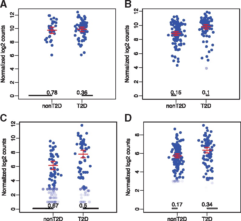
Examples of different forms of differential expression from the T2D dataset: (A) phase transition alone (Form I P-value = 4.41e-11, Form II P-value = 0.98); (B) magnitude regulation only (Form I P-value = 0.22, Form II P-value = 4.9e-06); (C) phase transition and magnitude regulation in concordant manner (Form I P-value = 8.42e-03, Form II P-value = 4.04e-05); (D) expression compensation (Form I P-value = 3.91e-03, Form II P-value = 1.61e-05). Each figure plots the expressions for a particular gene from all cells. The bars at the bottom of the figures represent the proportions of cells not expressing the gene (in Phase I). Each dot represents the log expression values for this gene from a cell. (P-values are from the proposed SC2P method)

These examples demonstrate the importance of identifying DE in both forms in order to gain a full understanding of the mechanism of DE. From our proposed method, SC2P reports the estimated proportions of cells in phase I/II, the fold change in phase II, and false discovery rate (FDR) associated with either type of DE, thus provides more comprehensive information for DE detection.

3.4 DE detection comparison with existing methods

We compare the DE detection performance of SC2P with several existing methods: SCDE (Kharchenko et al., 2014), BPSC (Vu et al., 2016) and MAST (Finak et al., 2015).

3.4.1. SC2P has higher sensitivity without sacrificing false discovery control

First, we validated the ability to identify known DE genes. There is a lack of gold standard for true positives in data, but more than 20 cell type marker genes are given in the human brain dataset. These marker genes are identified by comparing purified cell types via bulk RNA-seq (Darmanis et al., 2015; Zhang et al., 2014). They provide a partial list of true positives with strong signal, thus the ability to recover these genes among the top genes declared as DE is a reasonable validation of sensitivity.

Figure 4 shows the results from human brain dataset, comparing astrocytes and oligodendrocytes cells. Figure 4A compares the ability to recover known marker genes from the top ranked DE genes reported by four methods. Overall, SCDE, MAST and SC2P provide comparable overall results, and BPSC performs unfavorably. In addition, there are many more marker genes belonging to the Form I DE than Form II, indicating that the phase transition is more prevalent than magnitude adjustment between cell types. Even though SCDE reports these genes as DE, this mechanism is not revealed. The results for recovering DE in known markers in other comparisons are provided in Supplementary Material (neuron versus oligodendrocyte in Supplementary Fig. S3, and astrocyte versus neurons in Supplementary Fig. S4), and they lead to the same conclusion.

Fig. 4.

DE detection in human brain data, for astrocytes and oligodendrocytes comparison. Genes with FDR <0.05 from the statistical tests are deemed DE. (A) Recovery of known marker genes among top ranked DE genes; (B) Overlaps of DE genes in both forms from MAST and SC2P; (C) Assessment of type I error control based from permutation

We focus on the comparison with MAST hereafter since it is the only other method in the group that also provides the functionality of testing DE in two phases. Figure 4B shows MAST and SC2P identify many genes in common for both forms of DE, with SC2P being much more sensitive, when both methods control FDR at 0.05. To ensure that the high sensitivity of SC2P is not achieved by sacrificing the control of false discoveries, we performed the following permutation test to assess the type I error control from DE tests. We randomly shuffle the cells among two conditions, and then perform DE test on the shuffled dataset. All DE genes detected from the shuffled dataset should be false positives, and the resulting P-values from the DE test on shuffled dataset should follow uniform distribution. We then compute the observed type I error rate for a given P-value threshold, and compare that with the nominal P-value to evaluate the type I error control from the statistical test. Figure 4C shows that the observed type I errors based on a permutation test for both SC2P and MAST are well controlled and below the nominal type I error for both forms of DE detection, validating that the higher sensitivity of SC2P is not from inflated type I error. Comparison between other human brain cell types and the T2D data (Supplementary Figs S3–S6) lead to the same conclusion. These results show SC2P has better sensitivity than MAST, while having the comparable type I error control and accuracy in ranking genes.

We obtained the lists of different DE genes called by SC2P and MAST. The heatmap of these gene’s expression data are presented in Supplementary Figures S7 and S8. These figures provide a direct visualization of the raw data, thus are not obscured by the choice of modeling or processing, though they do not provide quantitative assessment of performance.

3.4.2. Robustness of SC2P

One critical property of any DE detection method is the robustness: that the discoveries are not sensitive to a few outliers. When we declare that a gene is differentially expressed between two cell populations, this result should not be driven by only a few cells. In other words, the analysis should be highly independent on the inclusion or exclusion a few cells, which are random samples from cell populations we study.

We compared the P-values obtained from the full dataset with the P-values from reduced dataset obtained by randomly removing 5% of the cells, from a population of 100 cells total in the neurons versus oligodendrocytes comparison. The panels in the second row of Figure 5 show excellent concordance between the two sets of P-values in DE detection from SC2P, in the testing of both forms of DE. In contrast, the panels in the first row of Figure 5 show such comparison results from MAST, which present substantial difference between results from the full data and reduced data. Most strikingly, we observe qualitatively different answers between the two sets of P-values: there are non-trivial amount of genes reported to have extreme statistical significance (with $\hspace{0.17em}{\text{log}}_{10}$P-value $\le -10$) when using all cell, but become non-significant (with log P-value near 0) when 5% cells are excluded. This contrast in robustness is observed in both DE in phase transition and in expression level within Phase II, in both datasets.

Fig. 5.

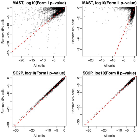
Robustness of DE detection. Figures show comparison of P-values from testing DE using all cells in the dataset or a subset with 5% cells randomly removed, in the human brain data (neurons versus oligodendrocytes). Form 1 (phase transition) and Form 2 (magnitude difference in phase II) DE are compared separately

We ran such analyses for 10 times, each time randomly selected 5% of the cells are removed. We observe that at least 5 out of the 10 times, the P-values from MAST show significant discordant. On the other hand, SC2P shows great consistence in all cases. The scatterplots for all 10 runs are provided as Supplementary Figure S9. We further perform additional analyses by removing 10, 20 and 50% cells. Each analysis is run 10 times. In each scenario, we compute the Pearson’s correlation coefficients of P-values before and after removing cells. The distributions of the correlation coefficients from MAST and SC2P are presented in Supplementary Figure S10. In all scenarios, SC2P has much higher correlations than MAST, indicating better robustness. These results show that compared to MAST, SC2P is much more robust to outlier cells, benefited from our method for estimating transcription phases.

3.4.3. Simulation

We conduct simulation studies to further compare the DE detection performances from MAST and SC2P. The simulated data are generated based on the human brain data so that they mimic the real data characteristics. The detailed simulation procedures and results are presented in Supplementary Material Section 8 and Supplementary Figures S13–S15. Overall, the simulation results are consistent with the real data results: SC2P are MAST provide comparable gene ranks, but SC2P is more sensitive due to better statistical inference.

3.4.4. Comparison with DESeq2

DESeq2 (Love et al., 2014) is a very popular tool for detecting DE genes in bulk RNA-seq data. Though it is not specifically designed for scRNA-seq, it is worth exploring its performance in scRNA-seq DE detection. We ran DESeq2 on the brain and T2D datasets and compared its performance with other methods. The results are presented in Supplementary Material Section 9 and Supplementary Figures S16–S20. In terms of recovering known marker genes, DESeq2 fell below the group of better performers (SCDE, MAST and SC2P) but was better than BPSC. DESeq2 tended to identify many more genes as DE at any FDR cutoff ranging from 1% to 20%, at a cost of inflated type I error. Though DESeq2 could discover many genes that were identified by SC2P or MAST or both, its observed type I error was much greater than nominal type I error, meaning it identified many more false positives than expected. In addition, since DESeq2 tests for the mean expression difference between groups, it does not reveal whether the form of DE involves phase transition. Overall, these drawbacks make DESeq2 undesirable for DE analysis for scRNA-seq data.

3.5 Computational performance

SC2P provides excellent computational performance. We profiled the times required for different methods to run DE analyses. All profiling was done on a MacBook pro laptop with i7 2.7 GHz CPU and 16 G RAM. When there are 100 cells in each group, SC2P takes 63.3 s, MAST takes 211.8 s and BPSC takes 3167.6 s. SCDE recommends to run on multiple cores. On a single core, it did not finish after five hours. So we focus on the comparison between SC2P and MAST. Table 1 summarizes the times (in seconds) required for different numbers of cells. Overall, SC2P is 2-3 times faster than MAST.

Table 1.

Time (in seconds) required for MAST and SC2P

# cells	100	200	500	1000	2000	5000
MAST	211.8	297.4	476.9	756.6	1214.6	2897.9
SC2P	63.3	85.7	160.0	285.3	574.4	1704.4

4 Discussion

Transcription is a complex process that is usually divided into three phases, including initiation (in higher eukaryotes, this is followed by the pause and release from pause of RNA Pol II), elongation and termination (Venkatesh and Workman, 2015). These steps are under regulation in various extent. The initiation, for example, involves intricate cooperation of multiple complexes in the disassembly of nucleosomes that creates a nucleosome-depleted region (NDR) which makes the DNA accessible to Pol II. Maintaining the NDR also allows multiple rounds of transcription to take place. Once initiated (and released from the pause), multiple factors affect the elongation speed, hence the production rate of RNA transcripts. The number of transcripts of a particular gene depends on both the production and degradation rate. Real-time measurements of transcription activity, taken from fluorescence in situ hybridization (FISH) in individual cells, indicate that genes transition between inactive and active states of transcription (Dar et al., 2012; Raj et al., 2006). The transition from inactive to active state leads to pulsatile expression patterns often referred to as bursting. As a result, we observe, in scRNA-seq data, gene expression counts that exemplify two modes of regulation: one mode that accounts for a binary transition from an inactive phase (Phase I) into an active, high expression phase (Phase II) and another mode that accounts for a regulation of the expression level within Phase II.

With bulk RNA-seq, the average expression of a large population of cells is measured, masking the heterogeneities among cells. scRNA-seq makes it possible to understand the transcriptional variation at the single cell level, providing evidence of bimodal expression regulation. However, the detection of DE has either remained as a comparison of the mean expression (Trapnell et al., 2014; Vu et al., 2016), or with arbitrary cut off for expression phases. In this work, we advocate that the DE test in scRNA-seq should be performed in both modes: phase transition and magnitude tuning. To achieve that, a vital first step is to accurately estimate the phases of expression for all genes in all cells. We present evidence that there are differences in overall detection rate among cells, and this is positively correlated with but different from the non-zero percentage (Supplementary Figs S10 and S11). This simple but effective method provides DE identification with increased sensitivity without sacrificing specificity, as well as greatly improved robustness. Furthermore, the results provide better interpretation of the DE regulation mechanism.

The excess of zero counts in scRNA-seq data is observed widely, though the source of these zero counts is debated. Some treat zero as unexpressed (Finak et al., 2015), others consider the zeros as technical dropouts and use imputation to recover the unobserved expression (Huang et al., 2017; Lin et al., 2017; Zhu et al., 2016). There are definitely technical dropouts, especially in low depth sequencing. On the other hand, the genome accessibility varies among cells (Buenrostro et al., 2015; Thurman et al., 2012) and transcription is certainly not active throughout the entire genome in a given cell. Therefore, we believe that both biological and technical reasons contribute to observed zero counts. Since scRNA-seq measures the quantity of RNA in a cell, not the transcription activity itself, even in inactive phase, there are RNA molecules already transcribed and not completely degraded. This is consistent with data from FISH experiments, in which cells without active transcription sites have fewer but non-zero reporter mRNA (Raj et al., 2006). Thus we argue that zero counts (as well as very low counts) are ‘lack of evidence’ for active transcription.

Existing threshold-based methods for phase determination fail to properly account for important data characteristics, including the variation of Phase I counts across cells. A major contribution of our method is providing data-driven thresholds that account for technical and biological factors, and both the cell- and gene-specific characteristics in the determination of expression status. Our current model only considers gene-specific factors in Phase II, while treating the Phase I parameters as if they were the same across genes. This is a choice for computational simplicity, as the variability due to Poisson counting at low counts makes it difficult to identify small difference in the Poisson rate. However, as public data accumulates, we will be able to observe a gene’s expression over a wide variety of conditions and in very large sample sizes. With multi-experiment databases we will be able to extend the model to estimate gene-specific patterns in both phases. Our long term goal is to establish gene-specific priors for both phases to accurately infer DE in cell- and gene-specific context. Such work on large scale databases have been presented on microarray platforms (McCall et al., 2011, 2014), which we predict will be greatly improved by single cell level data.

We model Phase II expression with a LNP distribution, instead of Gamma-Poisson (negative binomial), which is the most common choice for bulk RNA-seq data (Anders and Huber, 2010; Love et al., 2014; Robinson and Smyth, 2007; Wu et al., 2013). The Gamma distribution is often a choice of mathematical convenience and it is very similar to lognormal when the dispersion parameter is small, which is usually the case in bulk RNA-seq, since the expression level is an average over a large collection of cells. When the dispersion is small, both the dispersion parameter in the Gamma distribution and the parameter ${\sigma }^2$ in the lognormal distribution correspond to the square of the biological coefficient of variation (BCV) (Wu et al., 2013). However, when the CV is large and often exceeding 1 (Supplementary Material, Section 1), it would force the Gamma distribution to be extremely skewed and have a mode at 0, and lose its flexibility in shape. Using lognormal distribution to model the true expression rate not only allows better flexibility, but also allows easy extension to accommodate more complex study designs, such as mixed effects and nested design, by using existing methods for linear models on the log transformed data.

The datasets we tested do not use unique molecular identifiers (UMIs) (Islam et al., 2014; Kivioja et al., 2012), which are additional barcodes added to RNA transcripts before amplification. In UMI data, reads that map to a gene and share the same UMI are counted as originating from the same transcript, thus UMI data have much lower counts. Additional error correction of the UMIs in preprocessing may be necessary, and different normalization strategy is recommended (Stegle et al., 2015). These factors complicate the assessment of DE detection, and we have not included such comparison in this paper. The lower count level in UMI data makes it more difficult to decompose the two latent phases. At this stage, the current methods including SC2P may not work well for UMI data, or data with low depth sequencing, in terms of detecting DE in the form of phase changes.

Funding

This work was partially supported by NIH/NIGMS award R01GM122083 for HW, by R01GM122083, NSF DBI1054905, P20GM109035 for ZW. Single cell transcriptome work in the Stitzel Lab is supported by the Assistant Secretary of Defense for Health Affairs, through the Peer Reviewed Medical Research Program under Award No. W81XWH-16-1-0130. Opinions, interpretations, conclusions and recommendations are solely the responsibility of the authors, are not necessarily endorsed by the Department of Defense.

Conflict of Interest: none declared.

References

- Anders S., Huber W. (2010) Differential expression analysis for sequence count data. Genome Biol., 11, R106.. [DOI] [PMC free article] [PubMed] [Google Scholar]
- Bacher R., Kendziorski C. (2016) Design and computational analysis of single-cell RNA-sequencing experiments. Genome Biol., 17, 63.. [DOI] [PMC free article] [PubMed] [Google Scholar]
- Benjamini Y., Hochberg Y. (1995) Controlling the false discovery rate: a practical and powerful approach to multiple testing. J. R. Stat. Soc. Ser. B (Methodological), 57, 289–300. [Google Scholar]
- Buenrostro J.D. et al. (2015) Single-cell chromatin accessibility reveals principles of regulatory variation. Nature, 523, 486–490. [DOI] [PMC free article] [PubMed] [Google Scholar]
- Buettner F. et al. (2015) Computational analysis of cell-to-cell heterogeneity in single-cell RNA-sequencing data reveals hidden subpopulations of cells. Nat. Biotechnol., 33, 155–160. [DOI] [PubMed] [Google Scholar]
- Dar R.D. et al. (2012) Transcriptional burst frequency and burst size are equally modulated across the human genome. Proc. Natl. Acad. Sci. USA, 109, 17454–17459. [DOI] [PMC free article] [PubMed] [Google Scholar]
- Darmanis S. et al. (2015) A survey of human brain transcriptome diversity at the single cell level. Proc. Natl. Acad. Sci. USA, 112, 7285–7290. [DOI] [PMC free article] [PubMed] [Google Scholar]
- Delmans M., Hemberg M. (2016) Discrete distributional differential expression (d 3 e)—a tool for gene expression analysis of single-cell rna-seq data. BMC Bioinformatics, 17, 110.. [DOI] [PMC free article] [PubMed] [Google Scholar]
- Finak G. et al. (2015) MAST: a flexible statistical framework for assessing transcriptional changes and characterizing heterogeneity in single-cell RNA sequencing data. Genome Biol., 16, 278.. [DOI] [PMC free article] [PubMed] [Google Scholar]
- Grün D. et al. (2015) Single-cell messenger RNA sequencing reveals rare intestinal cell types. Nature, 525, 251–255. [DOI] [PubMed] [Google Scholar]
- Huang M. et al. (2017) Gene expression recovery for single cell RNA sequencing. doi: 10.1101/138677. [DOI] [PMC free article] [PubMed]
- Islam S. et al. (2014) Quantitative single-cell RNA-seq with unique molecular identifiers. Nat. Methods, 11, 163.. [DOI] [PubMed] [Google Scholar]
- Jiang L. et al. (2016) GiniClust: detecting rare cell types from single-cell gene expression data with Gini index. Genome Biol., 17, 144.. [DOI] [PMC free article] [PubMed] [Google Scholar]
- Jonkers I., Lis J.T. (2015) Getting up to speed with transcription elongation by RNA polymerase II. Nat. Rev. Mol. Cell Biol., 16, 167–177. [DOI] [PMC free article] [PubMed] [Google Scholar]
- Kharchenko P.V. et al. (2014) Bayesian approach to single-cell differential expression analysis. Nat. Methods, 11, 740–742. [DOI] [PMC free article] [PubMed] [Google Scholar]
- Kiselev V.Y. et al. (2017) SC3: consensus clustering of single-cell RNA-seq data. Nat. Methods, 14, 483–486. [DOI] [PMC free article] [PubMed] [Google Scholar]
- Kivioja T. et al. (2012) Counting absolute numbers of molecules using unique molecular identifiers. Nat. Methods, 9, 72.. [DOI] [PubMed] [Google Scholar]
- Korthauer K.D. et al. (2016) A statistical approach for identifying differential distributions in single-cell RNA-seq experiments. Genome Biol., 17, 222.. [DOI] [PMC free article] [PubMed] [Google Scholar]
- Lawlor N. et al. (2017) Single-cell transcriptomes identify human islet cell signatures and reveal cell-type–specific expression changes in type 2 diabetes. Genome Res., 27, 208–222. [DOI] [PMC free article] [PubMed] [Google Scholar]
- Lin P. et al. (2017) CIDR: ultrafast and accurate clustering through imputation for single-cell RNA-seq data. Genome Biol., 18, 59.. [DOI] [PMC free article] [PubMed] [Google Scholar]
- Love M.I. et al. (2014) Moderated estimation of fold change and dispersion for RNA-seq data with DESeq2. Genome Biol., 15, 550.. [DOI] [PMC free article] [PubMed] [Google Scholar]
- McCall M.N. et al. (2011) The gene expression barcode: leveraging public data repositories to begin cataloging the human and murine transcriptomes. Nucleic Acids Res., 39, D1011–D1015. [DOI] [PMC free article] [PubMed] [Google Scholar]
- McCall M.N. et al. (2014) The gene expression barcode 3.0: improved data processing and mining tools. Nucleic Acids Res., 42, D938–D943. [DOI] [PMC free article] [PubMed] [Google Scholar]
- Ntranos V. et al. (2016) Fast and accurate single-cell RNA-seq analysis by clustering of transcript-compatibility counts. Genome Biol., 17, 112.. [DOI] [PMC free article] [PubMed] [Google Scholar]
- Patel A.P. et al. (2014) Single-cell RNA-seq highlights intratumoral heterogeneity in primary glioblastoma. Science, 344, 1396–1401. [DOI] [PMC free article] [PubMed] [Google Scholar]
- Picelli S. et al. (2013) Smart-seq2 for sensitive full-length transcriptome profiling in single cells. Nat. Methods, 10, 1096–1098. [DOI] [PubMed] [Google Scholar]
- Raj A. et al. (2006) Stochastic mRNA synthesis in mammalian cells. PLoS Biol., 4, e309.. [DOI] [PMC free article] [PubMed] [Google Scholar]
- Ramsköld D. et al. (2012) Full-length mRNA-Seq from single-cell levels of RNA and individual circulating tumor cells. Nat. Biotechnol., 30, 777–782. [DOI] [PMC free article] [PubMed] [Google Scholar]
- Robinson M., Smyth G. (2007) Moderated statistical tests for assessing differences in tag abundance. Bioinformatics, 23, 2881–2887. [DOI] [PubMed] [Google Scholar]
- Shalek A.K. et al. (2013) Single-cell transcriptomics reveals bimodality in expression and splicing in immune cells. Nature, 498, 236–240. [DOI] [PMC free article] [PubMed] [Google Scholar]
- Shalek A.K. et al. (2014) Single-cell RNA-seq reveals dynamic paracrine control of cellular variation. Nature, 510, 363–369. [DOI] [PMC free article] [PubMed] [Google Scholar]
- Shekhar K. et al. (2016) Comprehensive classification of retinal bipolar neurons by single-cell transcriptomics. Cell, 166, 1308–1323. [DOI] [PMC free article] [PubMed] [Google Scholar]
- Smyth G.K. (2004) Linear models and empirical bayes methods for assessing differential expression in microarray experiments. Stat. Appl. Genet. Mol. Biol., 3, 1. [DOI] [PubMed] [Google Scholar]
- Stegle O. et al. (2015) Computational and analytical challenges in single-cell transcriptomics. Nat. Rev. Genet., 16, 133.. [DOI] [PubMed] [Google Scholar]
- Tang F. et al. (2009) mRNA-Seq whole-transcriptome analysis of a single cell. Nat. Methods, 6, 377–382. [DOI] [PubMed] [Google Scholar]
- Thurman R.E. et al. (2012) The accessible chromatin landscape of the human genome. Nature, 489, 75.. [DOI] [PMC free article] [PubMed] [Google Scholar]
- Trapnell C. et al. (2014) The dynamics and regulators of cell fate decisions are revealed by pseudotemporal ordering of single cells. Nat. Biotechnol., 32, 381–386. [DOI] [PMC free article] [PubMed] [Google Scholar]
- Usoskin D. et al. (2015) Unbiased classification of sensory neuron types by large-scale single-cell RNA sequencing. Nat. Neurosci., 18, 145–153. [DOI] [PubMed] [Google Scholar]
- Venkatesh S., Workman J.L. (2015) Histone exchange, chromatin structure and the regulation of transcription. Nat. Rev. Mol. Cell Biol., 16, 178.. [DOI] [PubMed] [Google Scholar]
- Vu T.N. et al. (2016) Beta-Poisson model for single-cell RNA-seq data analyses. Bioinformatics, 32, 2128–2135. [DOI] [PMC free article] [PubMed] [Google Scholar]
- Wills Q.F. et al. (2013) Single-cell gene expression analysis reveals genetic associations masked in whole-tissue experiments. Nat. Biotechnol., 31, 748–752. [DOI] [PubMed] [Google Scholar]
- Wu H. et al. (2013) A new shrinkage estimator for dispersion improves differential expression detection in rna-seq data. Biostatistics, 14, 232–243. [DOI] [PMC free article] [PubMed] [Google Scholar]
- Zhang Y. et al. (2014) An RNA-sequencing transcriptome and splicing database of glia, neurons, and vascular cells of the cerebral cortex. J. Neurosci., 34, 11929–11947. [DOI] [PMC free article] [PubMed] [Google Scholar]
- Zhu L. et al. (2016) A unified statistical framework for RNA sequence data from individual cells and tissue. arXiv preprint arXiv: 1609.08028.
Associated Data
This section collects any data citations, data availability statements, or supplementary materials included in this article.