Multi-speed Sedimentation Velocity Simulations with UltraScan-III

Abstract

Recent developments in the UltraScan-III software make it possible to model multi-speed analytical ultracentrifugation sedimentation velocity experiments using finite element solutions of the Lamm equation. Using simulated data, we demonstrate here how these innovations can be used to enhance the resolution of sedimentation velocity experiments when compared to single-speed experiments. Using heterogeneous systems covering as much as five orders of magnitude in molar mass and five-fold in anisotropy we compare results from runs performed at multiple speeds to those obtained from single-speed experiments, fitted individually and analyzed globally over multiple speeds, and quantify resolution for samples heterogeneous in size and anisotropy. We also provide guidance on the design of multi-speed experiments and offer a program that can be used to deduce optimal spacing of rotor speeds and speed step durations when a few parameters from the experiment can be estimated. These include the meniscus position, the sedimentation coefficient of the largest species in a mixture, and a solute distribution. Our results show that errors observed in the determination of hydrodynamic parameters for system with great heterogeneity are markedly reduced when multi-speed analysis is employed.

Introduction

When performing sedimentation velocity experiments we frequently encounter complex mixtures exhibiting significant heterogeneity. Examples include systems where protein analytes aggregate, degrade, or both processes occur at the same time, leading to mixtures that contain both large and small species that may vary significantly in their anisotropies and molar masses. In polymer chemistry, synthesis products often exhibit very large size ranges, which translate into broad range sedimentation and diffusion coefficient distributions. Isodesmically associating systems can exhibit very broad sedimentation coefficient ranges, as do complex biological systems such as heterochromatin [1], resulting in very challenging data analysis situations [2]. Such systems typically do not lend themselves to traditional finite element analysis because the disparate analytes have drastically different sedimentation speeds, sedimentation times, and diffusion properties which need to be discretized over very large ranges, leading to low resolutions in discretized parameters. In an effort to make heterogeneous sample analysis by finite element modeling more practical, we have implemented a rigorous multi-speed method protocol in UltraScan-III. The theory behind multi-speed simulation and analysis, and its implementation in UltraScan [3], a software package for the analysis of analytical ultracentrifugation (AUC) data from both the Beckman-Coulter Proteomelab XLA/XLI and the Optima AUC, has been discussed in a companion manuscript [4]. Multi-speed sedimentation velocity analysis promises to enhance the precision with which hydrodynamic parameters can be obtained from sedimentation velocity experiments by enhancing the hydrodynamic signal obtained in these experiments Here, we describe a strategy for multi-speed sedimentation velocity (SV) experimental designs and data analysis that is based on finite element solutions of the Lamm equation. As explained in [4], for heterogeneous mixtures that contain solutes exhibiting a large range of sedimentation and diffusion coefficients, the results are optimized when successively higher speeds are used to emphasize a range of hydrodynamically different components. Initially, a slow speed is used to collect sufficient diffusion signal for the largest species in the mixture, and sufficient scans can be measured before they pellet and are no longer visible in the solution column. Then the speed is raised, potentially multiple times, to provide optimal sedimentation coefficient resolution for successively smaller species. By using a multi-speed run profile, the sedimentation and diffusion signals are therefore enhanced for each species in a heterogeneous mixture, and this permits a more detailed analysis. It is reasonable to expect that different solutes can be detected in multiple speed steps, with overlap in the signal between different speed steps when the speeds are sufficiently closely spaced. This means that each speed step contributes some diffusion and sedimentation signal for each solute, as long as these species have not yet pelleted, or are not yet sedimented far enough to where the boundary is separated from the meniscus. Depending on the speed where solutes are measured, either sedimentation or diffusion signal will be enhanced, with no single speed providing both optimal sedimentation and optimal diffusion information for all species. In this work, we will show a) how to design a suitable speed profile for a heterogeneous mixture, and b) how a suitable finite element analysis method can exploit the sedimentation and diffusion signal available from multiple speed steps, and c) using simulated data, we compare the obtained result to the known parameters of the simulated system to quantify the additional information obtained.

Methods

1. Simulation

Simulated data provide realistic test conditions, including stochastic noise, that permit a systematic evaluation of the fitting method’s ability to retrieve information under conditions where rotor speed and experimental duration are varied and all other factors are held constant. This is useful since known input variables can be directly compared to the obtained results, and the effects of noise on the results and the limits of resolution such methods afford can be determined. To establish the value of multi-speed SV measurements, we simulated a mixture of five discrete components, at identical concentrations, which span five orders of magnitude in molar mass with identical partial specific volumes, and a simultaneous five-fold change in anisotropy. The simulation parameters are listed in Table 1.

Table 1.

Simulation parameters for a five component simulation model, spanning five orders of magnitude in molar mass and a five-fold change in anisotropy.

Parameter/Solute	Solute 1	Solute 2	Solute 3	Solute 4	Solute 5
s (× 1013 sec)	1.0111	2.3464	7.2608	25.276	93.858
D (× 107 cm2/sec)	18.862	4.3774	1.3545	0.47154	0.17509
Molar mass (Da)	5.0 × 103	5.0 × 104	5.0 × 105	5.0 × 106	5.0 × 107
f/f0	1.0	2.0	3.0	4.0	5.0
Absorbance	0.2	0.2	0.2	0.2	0.2
$\overline{\nu }\left(\text{ml}/\mathrm{g}\right)$	0.74	0.74	0.74	0.74	0.74

Simulation speeds were chosen to span the range of accessible speeds on the analytical ultracentrifuge, and to provide approximately a factor of 250-fold change in centrifugal force over all speeds. The experiment was simulated for 5 speed steps (3.8, 7.5, 15, 30 and 60 krpm), by simulating 100 equally spaced scans in time for each speed step. An acceleration time delay required for each speed step was added before the first scan was simulated, assuring that each scan originated from a constant speed as listed in Table 2. This replicates the constraints on an actual instrument, where due to technical reasons related to data acquisition, data can only be collected during a period of constant rotor speed. Hence, we simulated discrete speed steps rather than a continuous ramping of speed. For comparison, a 15,000 rpm single speed experiment control was simulated for the same composition, using otherwise identical simulation settings.

Table 2.

Simulation speeds and durations.

Speedstep:	1	2	3	4	5
Rotor speed (rpm):	3,800	7,500	15,000	30,000	60,000
Duration (hh:mm)	37:13	25:56	22:03	16:10	07:54
Delay (minutes):	0.167	0.167	0.317	1.875	1.875

Artificial stochastic noise of 0.4% of the total concentration was added to the simulation, to reflect a signal to noise ratio of 250, commensurate with values typically observed in the Beckman-Coulter Proteomelab XLA for a sample with a signal concentration of 1.0 absorbance units (AU). As in the companion manuscript [4], we chose a meniscus m of 5.9 cm to simulate a small air pocket above the meniscus, and a bottom of cell position of 7.2 cm at rest. Rotor stretch was added for each speed according to the rotor calibration of one of our An60Ti rotors, with stretch coefficients of s₁ = 1.20642 × 10⁻⁸ and s₂ = 5.29077 × 10⁻¹². The simulation assumed the density and viscosity of water at 20°C (as defined in UltraScan) and an acceleration rate of 400 rpm/sec. Compressibility of the solvent was not considered. All finite element solutions were simulated with the Adaptive Space-Time Finite Element Method (ASTFEM) for non-interacting, ideal solutes [5] using an initial number of 1000 radial points.

Speeds and durations for each speed step are listed in Table 2.

2. Experimental Design

Experimental designs require that the operator sets the rotor speed v and the duration t for a sedimentation velocity measurement. Given a rotor speed, t is optimally set to no less than the duration required for the midpoint of the boundary from each component with sedimentation coefficient s to sediment from the meniscus position m to the point where it would have crossed the bottom position b, were the cell infinitely long. This theoretical time can be calculated with Equ. 1

$$t=\ln \left(\frac{b}{m}\right)\frac{1}{s{\mathrm{\omega }}^2}$$ Equ. 1

where ω is the angular rotor speed. Clearly, for a heterogeneous system, each component in the mixture will have a different sedimentation coefficient, so t will be different for each species in a mixture. The first speed step should start with the lowest speed, and optimally describe the largest species in the system, and v₁ should be small enough and t₁ should be large enough to provide sufficient diffusion signal and to provide sufficient time for the detector to collect enough data. For the first speed step, v₁ and t₁ are therefore dependent on the largest species in the mixture. The next higher speed step should be chosen such that the second largest species is optimally measured, and sedimented to the bottom of the cell as calculated by Equ. 1. To best predict t₂, one must consider the sedimentation displacement for species 2 during the first speed step, and subtract that amount from the sedimentation still required for the boundary midpoint from species 2 to reach the bottom. Again, Equ. 1 is used to predict the time for each speed step. Subsequent speed steps follow the same principle, each species acquiring a new m from each speed step. The change in speed for each speed step depends on the s-value distribution in the experiment, which, if unknown, can be approximated from a single speed experiment. An exponential s-value distribution may require an exponential speed step distribution, while a more gaussian distribution may be adequately described by a linear increase in centrifugation force with each speed step. To facilitate the selection of the experimental duration and rotor speed for each step, we have written a small C++ program (SI 1) that takes the original meniscus, the largest s-value observed, and the starting and maximal rotor speed as a command line argument to predict appropriate rotor speeds and speed step durations for optimal speed step configurations.

3. Fitting approach for multi-speed data

When collecting data in multi-speed mode, UltraScan will separate each speed step into a separate experimental dataset. Each speed step must be analyzed initially as a separate experiment. While a global analysis of all speeds covering all solutes promises to combine the best of both sedimentation and diffusion signal, a non-interacting global analysis over all speeds as implemented in UltraScan is not appropriate in the general case, because it assumes that the overall number of solutes does not change, and that all solutes are measurable with a similar concentration in all speed steps. However, in the general case, it is possible that the largest components may have completely sedimented out of view during the later high-speed speed steps by pelleting during earlier speed steps. Similarly, very small components may not have sedimented enough at the slowest speeds to capture a sufficient boundary signal from them. Hence, a global fit for a very heterogeneous system where solutes may be missing at either end of the speed spectrum is not suitable. Nevertheless, a pseudo-global analysis is possible, where each speed step is analyzed individually over the entire expected sedimentation and anisotropy range, and results from all speed steps are merged into a global model, which can be further refined for each speed step depending on individual results obtained from each speed step.

The first step in the analysis consists of identifying the maximum s-value that needs to be considered in the range to be fitted. Here, the slowest speed step will contain the signal from the fastest sedimenting solutes, and should be used to determine the upper limit for all speed steps. Since all data collected in intensity mode will contain a considerable amount of time-invariant noise, this is best accomplished with the time-derivative method [6] implemented in UltraScan, which eliminates time-invariant noise by scan pair subtractions. To estimate the upper limit, a group of scans near the end of the first speed step is selected for analysis that still includes a stable plateau region. The point where the g*(s) distribution approaches zero on the high end of the sedimentation coefficient spectrum should be chosen for the cut-off. For the lowest s-value included in the fitting range a lower limit of 0.5 s is appropriate in most cases, unless prior knowledge suggests that the lowest s-value is higher, in which case an increase of the lower limit of the s-value range is preferred to improve resolution for the overall range. Frictional ratio ranges should be chosen based on prior knowledge of the system. If solutes are known to be globular, well-folded proteins, or spherical nanoparticles, a low range of 1-2 could be chosen for the anisotropy fitting range, otherwise higher frictional ratios should be included in the fitting range. For reference, a highly anisotropic molecule such as a 2,880 base pair linear DNA fragment in 100 mM NaCl approaches a frictional ratio limit of approximately 9 [7]. Data analysis with UltraScan is performed on parallel architectures [8], and the datasets from each speed should initially be analyzed with the same sedimentation and frictional ratio fitting range. The ASTFEM approach used for fitting by any method available in UltraScan [7, 9, 10, 11, 12] detects any solute already pelleted and will exclude those solutes automatically from the fit and simulation for higher speed steps [3]. Initially, a two-dimensional spectrum analysis (2DSA) [9, 10] is performed to remove time-invariant noise contributions. Next, 2DSA is used to fit the meniscus positions [13], simultaneously fitting both time- and radially-invariant noise contributions. This is followed by an iterative 2DSA refinement step, also performed with time- and radially-invariant noise removal. In the final step a 2DSA-Monte Carlo (2DSA-MC) analysis is performed [14]. At this point, a comprehensive fit for each speed step is available from the 2DSA-MC models. For a global interpretation of the multi-speed dataset, it is recommended that the 2DSA-MC models from all speed steps are merged into a global model, which can be visualized in the pseudo-3D viewer in UltraScan. The combined model then reflects all species present in the entire experiments, regardless of speed step. If a few discrete species are identified in this model, rather than a broad distribution, a manual initialization of a genetic algorithm (GA) analysis is recommended. This is accomplished by drawing limit regions (referred to as “buckets” in the software) around areas of signal in the 2-dimensional domain (see Figure 1A). The obtained initialization file is then used to perform a GA-Monte Carlo (GA-MC) analysis. In this approach each bucket will be fitted to result in a single solute. By performing a Monte Carlo analysis on top of the GA analysis, the noise in the experimental data is explored, and 95% confidence limits for each parameter describing individual solutes will be available [14]. The same GA initialization file is then used to repeat the GA-MC fit for each individual speed step separately.

Figure 1.

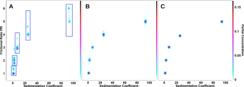
Combined results for 2DSA and GA-MC analyses. A: Global overlay model for all speeds of the 2DSA-MC analyses of the simulated 5-component system. Blue lines represent the GA initialization limits used for the GA-MC analysis. B: 2DSA-MC analysis model using only the optimal solute from each speed step, clearly showing better distribution statistics than the overlay of all models. Either one can be used to initialize the GA analysis. C: Final GA-MC analysis model using only the optimal solute from each speed step, producing nearly identical values as the simulated input parameters (within 1 % error of the original values).

4. Analysis and result interpretation

For simulated data, we have prior knowledge of the simulation parameters used to generate the test data. Therefore, we have a good metric to judge the quality of the results by comparing the obtained values to the actual values obtained for the parameters describing a solute. One intuitive and convenient metric is the solute’s molar mass M, given by:

$$M=\frac{\mathit{sRT}}{D\left(1-\overline{\nu }\mathrm{\rho }\right)}$$ Equ. 2

where R is the gas constant, T the temperature, ρ the density of the solvent, and is the partial specific volume of the solute. The molar mass captures both the sedimentation and diffusion coefficients of the solute, the primary signals measured in the sedimentation velocity experiment. Since the partial specific volume is given, the molar mass represents the quality of the information retrieved from the experiment. A second parameter that is useful to describe the properties of the molecule is the anisotropy, expressed in terms of the frictional ratio, f/f₀, which is not a true hydrodynamic parameter, but a measure of the globularity of the particle, which is 1.0 for a perfect sphere and larger for non-spherical particles. It has M, D and dependence, and is given by Equ. 3.

$$\frac{f}{f_0}=\frac{RT}{ND}\left[6\mathrm{\pi }\mathrm{\eta }{\left(\frac{3M\overline{\nu }}{4\mathrm{\pi }N}\right)}^{1/3}\right]$$ Equ. 3

where N is Avogadro’s number, f the frictional coefficient of the solute, and f₀ the hypothetical frictional coefficient of a spherical particle with the same partial specific volume as the sedimenting solute. The final fitted parameter of interest is the partial concentration of each solute. Since we added realistic stochastic noise to the simulated data, we do not expect a unique solution, but rather a range of values from a Monte Carlo analysis. The metrics we chose to compare the performance of multi- and single-speed analysis include the percent error observed from the means of the Monte Carlo parameter distributions (Equ. 4)

$$\mathrm{\%}\mathit{\text{Error}}=100\mathrm{\%}\cdot \left[\frac{\sqrt{{\left(X_e-X_m\right)}^2}}{X_e}\right]$$ Equ. 4

where X_e is the expected simulated parameter, and X_m is the observed mean from the Monte Carlo distribution, and the average 95% confidence interval (CI) error from each Monte Carlo parameter distribution (Equ. 5)

$$95\mathrm{\%}CI\mathit{\text{Error}}=100\mathrm{\%}\cdot \left[\frac{\left(\sqrt{{\left(X_e-X_{95l}\right)}^2}+\sqrt{{\left(X_e-X_{95h}\right)}^2}\right)/2}{X_e}\right]$$ Equ. 5

where X_95l and X_95h are the low and high 95% confidence intervals, respectively.

Results

The simulated system investigated here was selected to represent a mixture of discrete, non-interacting species, spanning a large range of molar masses and anisotropies. We tried to resolve a mixture containing five different molecules present at equal concentration. Such a system is suitable for analysis by both 2DSA and GAs. Either method can be combined with a Monte Carlo analysis to derive fitting statistics for this system as discussed above. For all fits performed for both methods, the root mean square deviations (RMSD) obtained consistently matched the simulated stochastic noise level, with perfectly random residuals in all cases. When 2DSA-MC analysis results were combined into a global model, a pseudo-3D representation of this model suggested 5 discrete species (see Figure 1A), allowing us to define limited regions from the two-dimensional parameter space to be analyzed by GA-MC analysis. As anticipated, inspection of the individual speeds provided even better defined limits when speeds were optimally matched for a given solute. This is shown in Figure 2 and can be readily observed from the percent errors when the fitted parameter means were compared to the simulated input parameters. Figure 3 shows the percent errors for molar mass, frictional ratio, and total concentration obtained for each individual speed from the multi-speed experiment. From these results it is clear that each speed highlights a different solute optimally. Figure 1B demonstrates the pattern obtained from 2DSA-MC analysis when only the species with the smallest 95% confidence limit is selected from each speed step. As can be seen from Figure 1C, after GA-MC analysis based on the initialization shown in Figure 1A, a nearly identical pattern is obtained as in Figure 1B, but each solute is even more narrowly defined, attesting to the robustness of both methods. The percent error obtained when comparing the simulation parameters with the means of the parameter distributions for molar mass, frictional ratio, and partial concentration are shown for both 2DSA-MC and GA-MC analysis in Figure 3. From these results it is evident that for each speed step typically only one solute produces an error less than 1%, while the percent error for the other solutes from the same speed step can be significantly higher. Importantly, the single best reproduced species is different for each speed step, therefore, when all speed steps are considered, each species can be defined with a very low error. A very similar result is seen when the 95% confidence intervals for these parameters are compared. These can be computed for the parameter distributions from the molar mass and the frictional ratio (see Figure 4). As anticipated, here again the highest confidence is typically only obtained for one of the species of a speed step, but this species is a different one for each speed step, providing a reliable metric to identify the best speed for a given range of solutes in a mixture where the percent confidence interval is lower than that of the more poorly defined species. This pattern is revealed by the parabolic shape of the bar graphs in Figure 4. The 2DSA-MC analysis returned 95% confidence intervals with less than 25% deviation from the mean, and those returned by GA-MC analysis were less than 5% from the mean for the most well-defined species for any particular speed. Based on the 95% confidence intervals, the GA-MC results are, on average, 29% better than the 2DSA-MC results due to the lower degrees of freedom employed in the analysis. It should also be noted that the frictional ratio absolute confidence limits are lower than those from the molar masses, primarily due to the larger scale on which the molar mass is measured (across five orders of magnitude). Finally, we evaluated the overall benefit of using multi-speed analysis by comparing the multi-speed results to a standard single speed, 8-hour, 15 krpm experiment that was simulated for the same 5-solute system. The 2DSA-MC result for the single-speed experiment is shown in the lower right panel of Figure 2, the quantitative comparison for 2DSA-MC and GA-MC is shown in Figure 5. Regardless of method or parameter compared, the multi-speed experiment significantly outperforms the single-speed experiment. Based on the 95% confidence intervals of the Monte Carlo distributions, the multi-speed 2DSA-MC analysis shows a 54% improvement over the single-speed experiment, while the GA-MC analysis performs 60% better for the multi-speed experiment when optimally defined solute regions are considered in the multi-speed experiments.

Figure 2.

2DSA-MC results for individual speed steps. At each speed a different solute is optimally measured, and incurs the narrowest confidence limits (blue arrow). Lower right: 2DSA-MC result for a regular single speed experiment (15 krpm).

Figure 3.

Percent error statistics for the 2DSA-MC (red) and GA-MC (green) analyses for each of the speed steps when comparing mean values obtained from the analysis to simulation values (see Equ. 4). Top row: molar mass errors; center row: frictional ratio errors; bottom row: partial concentration errors. ND – species not detected due to having sedimented out of view.

Figure 4.

95% confidence interval statistics for the 2DSA-MC (red) and GA-MC (green) analyses for each speed step. Reported here are the average 95% confidence interval values obtained by comparing upper and lower limits of the 95% percent confidence intervals (see Equ. 5). Top row: molar mass errors; bottom row: frictional ratio errors. ND – species not detected due to having sedimented out of view. Due to the reduced number of degrees of freedom in the GA-MC fit the 30 and 60 krpm 95% confidence limits are near zero and not visible on the presented scale.

Figure 5.

95% confidence interval comparison between multi-speed (green) and single-speed (red) experiments for the molar mass (top) and frictional ratio (bottom) from 2DSA-MC (left) and GA-MC results.

Taken together, these results clearly show the significant benefit of multi-speed analysis which allows the investigator to obtain much higher precision and accuracy for heterogeneous samples. While on average the GA-MC analysis performed slightly better on optimally defined species and those in their vicinity at a given speed step, 2DSA-MC results provided a virtually identical pattern of individually well-matched species at different speeds, just showing slightly higher 95% confidence intervals. Obviously, percent error values are not available for actual experiments, but as can be seen from these results, the 95% confidence intervals are well suited to guide the user in determining which speed step provides the most reliable information for a subset of species present in a mixture. Variable speed profiles can be programmed easily in the new Optima AUC, in the older Proteomelab XLI/A it is also possible, with some restrictions, to accomplish a similar variable speed profile by using the equilibrium method setups. Additional experimental work will be necessary to validate our results, with particular focus on situations where solvent compressibility will affect boundary conditions for finite element solutions of the Lamm equation when the rotor speed is changed mid-run. While the analysis effort is somewhat greater for a multi-speed experiment, the gain in accuracy and precision promise to make multi-speed analysis a worthwhile approach for sedimentation velocity experiments of heterogeneous systems with broad distributions in sedimentation coefficients and diffusion coefficients.

References

- 1.Rogge RA, Hansen JC. Sedimentation Velocity Analysis of Large Oligomeric Chromatin Complexes Using Interference Detection. Methods Enzymol. 2015;562:349–62. doi: 10.1016/bs.mie.2015.05.007. Epub 2015 Jun 29. [DOI] [PubMed] [Google Scholar]
- 2.Ma J, Zhao H, Sandmaier J, Alexander Liddle J, Schuck P. Variable Field Analytical Ultracentrifugation: II. Gravitational Sweep Sedimentation Velocity. Biophys J. 2016 Jan 5;110(1):103–12. doi: 10.1016/j.bpj.2015.11.027. [DOI] [PMC free article] [PubMed] [Google Scholar]
- 3.Demeler B, Gorbet G. Analytical Ultracentrifugation Data Analysis with UltraScan-III. Ch 8. In: Uchiyama S, Stafford WF, Laue T, editors. Analytical Ultracentrifugation: Instrumentation, Software, and Applications. Springer; 2016. pp. 119–143. [Google Scholar]
- 4.Gorbet GE, Mohapatran S, Demeler B. Multi-Speed Sedimentation Velocity Implementation in UltraScan-III. Eur Biophys J. 2018 doi: 10.1007/s00249-018-1297-z. current issue. [DOI] [PMC free article] [PubMed] [Google Scholar]
- 5.Cao W, Demeler B. Modeling analytical ultracentrifugation experiments with an adaptive space-time finite element solution of the Lamm equation. Biophys J. 2005;89(3):1589–602. doi: 10.1529/biophysj.105.061135. [DOI] [PMC free article] [PubMed] [Google Scholar]
- 6.Stafford W. Boundary analysis in sedimentation transport experiments: A procedure for obtaining sedimentation coefficient distributions using the time derivative of the concentration profile. Anal Biochem. 1992;203:295–301. doi: 10.1016/0003-2697(92)90316-y. [DOI] [PubMed] [Google Scholar]
- 7.Gorbet G, Devlin T, Hernandez Uribe B, Demeler AK, Lindsey Z, Ganji S, Breton S, Weise-Cross L, Lafer EM, Brookes EH, Demeler B. A parametrically constrained optimization method for fitting sedimentation velocity experiments. Biophys J. 2014;106(8):1741–1750. doi: 10.1016/j.bpj.2014.02.022. [DOI] [PMC free article] [PubMed] [Google Scholar]
- 8.Brookes EH, Demeler B. Parallel computational techniques for the analysis of sedimentation velocity experiments in UltraScan. Colloid Polym Sci. 2008;286:138–148. [Google Scholar]
- 9.Brookes E, Boppana RV, Demeler B. Computing Large Sparse Multivariate Optimization Problems with an Application in Biophysics. Supercomputing ’06. 2006 ACM 0-7695-2700-0/06. [Google Scholar]
- 10.Brookes E, Cao W, Demeler B. A two-dimensional spectrum analysis for sedimentation velocity experiments of mixtures with heterogeneity in molecular weight and shape. Eur Biophys J. 2010;39(3):405–14. doi: 10.1007/s00249-009-0413-5. [DOI] [PMC free article] [PubMed] [Google Scholar]
- 11.Brookes E, Demeler B. Parsimonious Regularization using GAs Applied to the Analysis of Analytical Ultracentrifugation Experiments. GECCO Proceedings. 2007 ACM 978-1-59593-697-4/07/0007. [Google Scholar]
- 12.Demeler B, Nguyen TL, Gorbet GE, Schirf V, Brookes EH, Mulvaney P, El-Ballouli AO, Pan J, Bakr OM, Demeler AK. Hernandez Uribe BI, Bhattarai N, and RL Whetten. Characterization of Size, Anisotropy, and Density Heterogeneity of Nanoparticles by Sedimentation Velocity. Anal Chem. 2014 Aug 5;86(15):7688–95. doi: 10.1021/ac501722r. [DOI] [PMC free article] [PubMed] [Google Scholar]
- 13.Demeler B. Methods for the Design and Analysis of Sedimentation Velocity and Sedimentation Equilibrium Experiments with Proteins. Cur Protoc Prot Sci. 2010 doi: 10.1002/0471140864.ps0713s60. Chapter 7: Unit 7.13. [DOI] [PMC free article] [PubMed] [Google Scholar]
- 14.Demeler B, Brookes EH. Monte Carlo analysis of sedimentation experiments. Colloid Polym Sci. 2008;286:129–137. [Google Scholar]
Associated Data
This section collects any data citations, data availability statements, or supplementary materials included in this article.