Functional connectomics from neural dynamics: probabilistic graphical models for neuronal network of Caenorhabditis elegans

Abstract

We propose an approach to represent neuronal network dynamics as a probabilistic graphical model (PGM). To construct the PGM, we collect time series of neuronal responses produced by the neuronal network and use singular value decomposition to obtain a low-dimensional projection of the time-series data. We then extract dominant patterns from the projections to get pairwise dependency information and create a graphical model for the full network. The outcome model is a functional connectome that captures how stimuli propagate through the network and thus represents causal dependencies between neurons and stimuli. We apply our methodology to a model of the Caenorhabditis elegans somatic nervous system to validate and show an example of our approach. The structure and dynamics of the C. elegans nervous system are well studied and a model that generates neuronal responses is available. The resulting PGM enables us to obtain and verify underlying neuronal pathways for known behavioural scenarios and detect possible pathways for novel scenarios.

This article is part of a discussion meeting issue ‘Connectome to behaviour: modelling C. elegans at cellular resolution’.

1. Introduction

A probabilistic graphical model (PGM) is a statistical model in which a graph maps the conditional dependence structure between multiple random variables [1–3]. Construction of a PGM has been shown as an effective methodology for retrieving dominant trends and analysing events with very large numbers of dependent variables. Applications of graphical models has revolutionized a number of fields such as medical diagnosis, natural language processing and computer vision. The nodes of the PGM correspond to variables in a domain, and edges correspond to probabilistic interactions (conditional dependencies) between the variables. The most commonly used graphical models are Bayesian networks and Markov random fields. Bayesian networks are directed graphs parameterized by conditional probability distributions (CPDs), whereas Markov random fields are non-directed graphs parameterized by factors.

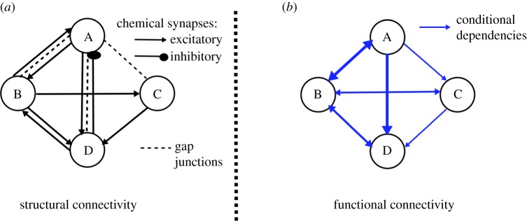
PGMs were successfully applied to problems for which direct inference is intractable [2]. It is thereby appealing to apply them in the context of neuronal network functionality. However, classical approaches for learning PGM structure are designed for discrete variables and are not compatible with neuronal networks consisting of dynamic neurons interacting through dynamic connections. Both neurons and their connections are typically modelled as nonlinear processes. A possible adaptation of a neuronal network to a statistical model, which captures functionality, is to consider each neuron as a random variable that takes values representing the states of the neuron. For simplicity it is often assumed, and here we assume it as well, that each neuron activity is binary-valued, with 0 being the inactive state and 1 being the active state. The PGM of a neuronal network is thereby a graph with neurons being the nodes and their dependencies being the edges (as demonstrated in figure 1).

Figure 1.

Representation of a neuronal network as a graphical model. (a) Example of structural/anatomical connectivity map in which nodes denote neurons and edges map connections, e.g. chemical synapses and electrical gap junctions. Interactions between neurons produce a nonlinear network that dynamically transports stimuli to neuronal behaviours. (b) Example of PGM constructed from the neuronal network governed by the structural connectivity map and nonlinear dynamics. In the PGM, nodes are random variables corresponding to neuronal states and edges are conditional probabilities. PGM structure captures functionality of the network and hence is typically different from the anatomical connectivity map. (Online version in colour.)

There are two main difficulties in learning a graphical model from dynamics. (i) Difficulty in estimating input–output correlations for a network whose responses are time-dependent. (ii) High dimensionality and complexity of neuronal networks typically incorporating recurrent structures. These factors make statistical inference hard to realize. Relevant work has been done in dynamic networks using either experimental data, such as [4–6], or simulated data, such as [7]. In both cases, ‘snapshots’ that record network dynamics are used to analyse time-series data. For estimating input–output correlations, statistical methods are applied to measure pairwise node correlation. For example, Honey et al. [7] proposed to use transfer entropy to capture patterns of directed interaction and information flow between pairs of nodes. Butte & Kohane [8] used entropy of gene expression patterns and the mutual information between RNA expression patterns for each pair of genes to compute pairwise mutual information. To address the problem that the network responses are time-dependent, works assuming that the underlying network is time-invariant, such as [4,9], or that estimate a sequence of graph structures such as [5,6], have been proposed.

It is also possible to use a machine learning approach, such as to sample the neuronal network multiple times as training data, and to evaluate candidate models according to a scoring function and search for the optimal model [1]. One of the drawbacks of score-based approaches is that in high-dimensional and cyclic neuronal networks, the problem of finding an optimal solution becomes NP-hard. Additional approaches have been employed for Bayesian network modelling for human functional network analysis. Zhang L. et al. and Zhang J. et al. introduced Dynamic Bayesian Networks, the Dynamic Bayesian Variable Partition Model and Dynamic Causal Modelling for fMRI time-series snapshots [10,11]. In these models, an underlying assumption for the time series is a Gaussian model, which does not apply for attractor neural dynamics generically appearing in the neuronal networks and require extensive computational cost. While more efficient approaches have been introduced, they still incorporate non-generic assumptions such as low-rank and sparsity of the responses [12].

Here, we propose a different approach that circumvents these complexities. As neurons are random variables, mathematically our approach is based on the concept that if we stimulate them using independently and identically distributed process, then the construction of the dependencies would be based on measuring how network response deviates from the stimuli distribution. Here, we use a simple distribution, the delta distribution, which is single neuron excitation, and record network response to each stimulus. Such an approach is simple to implement with simulated neural dynamics and potentially realizable with the rapid advance of optogenetic technologies to record and stimulate networks at a single neuron resolution [13]. While we employ a single excitation in our proposed algorithm, theoretically the approach is not limited to this stimulation and other distributions of the stimuli can be used. The required assumption is that stimulation of each neuron is independent and the outcome PGM superimposes response dynamics to independent experiments into a model.

To construct the graph, our key idea is to learn the dependencies from low-dimensional projections of time series instead of learning from sampled data directly. The low-dimensional representations capture the dominant dynamics of the network and thus reduce the complexity of the learning algorithm and the computational cost. To be able to capture the dominant patterns, we sample the network over a sufficiently long period such that we have captured the typical and dominant dynamics, i.e. the network converged to attractor dynamics, if such dynamics exist. Using this approach, we construct a PGM (a Bayesian network) that maps the functional connectivity between the neurons. The model can be used to ‘query’ the system given evidence regarding activity of some neurons or infer typical relation between activity of neurons. We define these concepts and explain the procedures for these tasks in §2 (figure 1).

We apply our method to the neuronal network of Caenorhabditis elegans to validate the PGM. Caenorhabditis elegans is a well-studied organism; the somatic nervous system of C. elegans consists of 279 neurons and the wiring diagram between these neurons was compiled by Varshney et al. consisting of 6393 chemical synapses, 890 gap junctions and 1410 neuro-muscular junctions [14]. In addition, experimental electrophysiological and optogenetic techniques for stimulating and recording neural activity in vivo and in situ have been introduced for C. elegans [15–17]. The connectome representing weights of dynamic interactions between neurons combined with a biophysical model of neural dynamics and their interactions enables us to simulate the full nervous system model [18–21]. In the following sections, we construct a Bayesian network that represents the functional connectivity of the neuronal network of C. elegans and verify the results with experimental data.

2. Construction of probabilistic graphical model from neuronal network dynamics

We first introduce the components of the Bayesian network in the context of neuronal networks. We then illustrate how conditional probabilities are assigned from the simulated neural dynamics. Finally, we show how computed probabilistic dependencies are used for the construction of a Bayesian network.

(a). Representing neuronal distributions with Bayesian networks

A Bayesian network is a representation of a joint probability distribution using a graph structure G = (V, E) and CPDs θ. The graph structure G is a directed acyclic graph whose vertices, V, correspond to random variables {X₁, X₂, …X_n}, and edges, E, correspond to connections between random variables, i.e. conditional dependencies. For each variable, θ describes the CPD given its parents in G. By applying the probability chain rule and using properties of conditional independence, joint probability distribution can be decomposed into the product form

where Pa^G(X_i) is the set of parents of X_i in G.

PGM is based on this property and graphically reformats probability distributions into a graph with parent and children nodes. For neuronal networks, each X_i corresponds to an individual neuron where each of them takes discrete values. Thus, we can represent P(X_i|U₁, …, U_k) as a table that specifies the probability of values for a neuron X_i for each joint assignment to its parent neurons U₁, …, U_k [4]. In the simplest case, we only consider pairwise conditional probability P(X_i = s_l | X_j = s_k), where neuron X_j receives input that drives it to a neural state s_k out of a set of states s = {s₁, .., s_k, .., s_m}, and we would like to estimate the probability of neuron X_i being in state s_l subject to evidence that X_j is in state s_k.

The structure of the PGM is designed to conveniently map the statistical dependencies to allow us to ‘query’ the graph in an efficient way. The query procedure, called posterior inference, uses the constructed PGM to provide information about probabilities of particular variables and their states, taking into account evidence regarding the states of other variables, i.e. conditional probability. In particular, there are two types of posterior inference tasks in the context of network pathways that can be answered using a graphical model. The first task is to infer conditional probabilities of the type P(Y | E = e), where the probability distribution over the values y ∈ Y, conditioned on E = e is inferred. For example, in such a case, functional pathways from upstream neurons (E) to downstream neurons (Y) can be inferred. The second task is to infer the maximum a posteriori (MAP) probability: , where the most probable assignment to the variables in Y is sought given the evidence E = e. In this task, functional pathways can be inferred through an inverse process, where downstream neurons (E) states are provided (E = e) and inference provides most probable upstream neurons (Y) with states (Y = y). PGM is capable of discovering the unstructured information within the distributions as it turns complex distributions into structured information that can be analysed effectively and efficiently using statistical tools. The benefit of using a PGM as the functional connectome is that posterior inference can be performed efficiently and circumvent the complexities in direct inference of response pathways in dynamic neuronal networks. In particular, posterior inference reveals the relations and pathways between known stimuli and downstream neurons or allows us to discover the stimuli that would trigger downstream neurons.

(b). Collecting data from simulated dynamics

We propose to find conditional probabilities for all pairs of neurons by simulating the network and recording data in snapshot matrices. The snapshot matrix represents finite time series of whole network dynamics for a particular input to a single neuron. The matrices are computed by injecting a constant input into every neuron in the network independently, thus resulting in a total of n matrices for the network of n neurons. Network dynamics are modelled by a set of dynamic equations, e.g. conductance-based model, which describe the biophysical processes of neurons and interactions between neurons. A snapshot matrix has the structure S = [S(t₀) S(t₁) … S(T)] of dimensions n × T, where n is the total number of neurons in the network and T is the length of the time span.

(c). Dimension reduction

We process the time-series data by projecting it into a lower-dimensional space using singular value decomposition (SVD). The benefits of SVD include reducing dimensionality and thus reduction of computational cost and robustness to noise [22]. Furthermore, when the SVD-based approach is applied to multi-node time-series network dynamics, it decomposes the data into spatial modes and their associated time-dependent coefficients. The spatial modes are orthogonal vectors representing activity patterns of the nodes [23]. When the recorded data have been conditioned on a particular event, each spatial mode vector is effectively a vector containing a response score for each node. As the spatial modes are ranked by singular values to reflect their dominance, the combination of dominant modes will include the most dominant combination of scores as a response to the event. This is the property that we use here to estimate dependence between stimulation and network response. Such an approach is more beneficial than direct estimate of statistical dependence (e.g. correlation) as it separates spatial and time-dependent data and ranks the spatial modes. Furthermore, these properties of SVD ensure that the estimation of the dependencies is robust with respect to sample time as long as they have captured the full dynamics to which the network converges.

More precisely, SVD of an n × p matrix S has the form

where U and V are n × n and p × p unitary matrices, with the columns of U spanning the column space of X (spatial neuronal modes) and the columns of V spanning the row space (time-dependent coefficients) [24]. Σ is assumed to have diagonal entries σ_j which are non-negative and in descending order, i.e. σ₁ ≥ σ₂ ≥ … s ≥ σ_m ≥ 0, where . Once the original matrix S is decomposed, U_j (column vector of U) and V_j (column vector of V) record the mode corresponding to singular value and temporal coefficients corresponding to the σ_j, respectively. Each singular value σ_j in Σ corresponds to the significance of the corresponding mode. Using SVD, we can find a lower-dimensional representation for the matrix S, which captures the dominant features of neural dynamics. Dimension reduction is performed by retaining k-dimensional subspace, where k < n, spanned by k-modes corresponding to top k singular values.

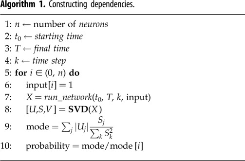
When using SVD to obtain a low-dimensional representation of the data, we need to retain enough modes to approximate the data. In practice, an energy criterion on singular values is often used as it specifies the amount of energy included in the chosen modes. For example, a typical energy criterion requires 95% of the energy in Σ. That is, the sum of the squares of the retained singular values should be at least 95% of the sum of the squares of all singular values. For a snapshot matrix whose network responses reach a fixed point, the first dominant mode would be sufficient to represent the fixed point. For oscillatory networks, the first two modes together represent oscillatory dynamics. Instead of using the classical k-rank approximation, we propose a new approach that takes the linear combination of the modes according to their significance, which results in a one-dimensional column vector. Specifically, we use the sum of all modes weighted by singular values as a one-dimensional representation of the original data (figures 2 and 3).

Figure 2.

Construction of dependencies between nodes. By injecting input stimuli into each neuron, we obtain a series of snapshot matrices that record network dynamics. By decomposing the snapshot matrices using SVD, we obtain the decomposition modes and compress them into a single vector for each matrix. We then normalize the vector according to its input neuron and obtain pairwise responses, which constitute the adjacency matrix of pairwise conditional probabilities.

Figure 3.

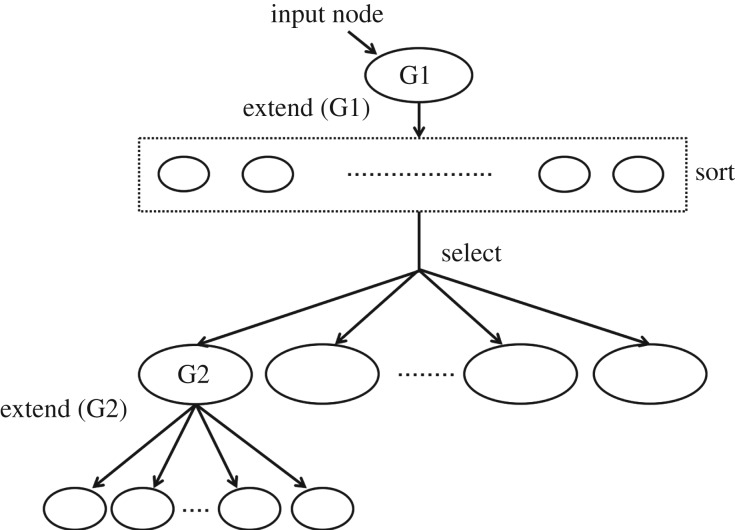
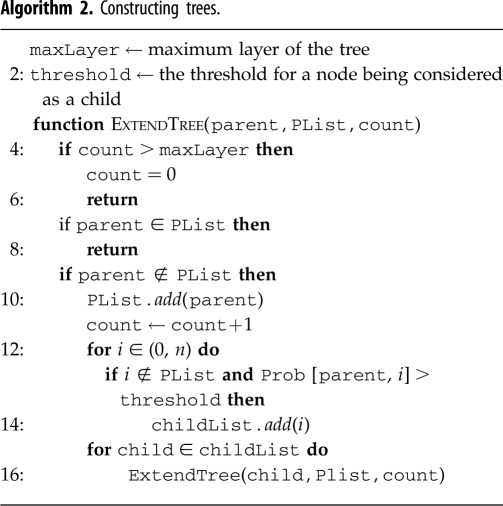
Tree construction from adjacency matrices. We start with the input node, and sort the other nodes according to their probabilities conditioned on the input node. We ignore nodes with conditional probabilities lower than the threshold, and select the top nodes with the highest conditional probabilities. A constraint can be imposed to limit the number of children that a node can have. From there we extend each node recursively, until it either reaches the maximum tree depth, or reaches neurons in a particular set (e.g. motor neurons). The threshold, maximum tree depth and maximum number of children are pre-set parameters to limit the size of the tree.

(d). Construction of a Bayesian network

The features extracted from snapshot matrices are used to obtain pairwise dependencies. Each snapshot matrix corresponds to a stimulation of a single neuron. We assume the stimulated neuron is driven into an active state and thus the snapshot matrix reflects the response of other neurons, which we transform to probabilities, conditioned on the stimulated neuron being activated. We achieve this by normalizing each mode according to the response of its input neuron, X_i. We interpret the result as the conditional probability P(X_j = 1 | X_i = 1) and store it into the ith column of the conditional probability table. The PGM itself consists of probabilities and thus does not indicate whether it is positive causality or negative (anti-)causality. Additional descriptive states of neuron activity could be added in the future by extending neural states, for example, each node state would be active, anti-active and inactive. P(X_j = 0 | X_i = 1) can be calculated by 1 − P(X_j = 1 | X_i = 1), and we assume that P(X_j = 0 | X_i = 0) = 1 and P(X_j = 1 | X_i = 0) = 0, i.e. a node cannot be active if there is no input into the network.

The resulting table is an n × n dependency matrix, which records the complete pairwise dependencies for the entire neuronal network (see figure 2). The matrix itself contains useful information about the network, and by constructing the PGM we can further extract and visualize this information. As any joint distribution can be decomposed into a product of conditional probabilities, the dependency matrix when transformed into pairwise conditional distributions records the full joint distributions encoded by the PGM. A natural graphical representation of a neuronal network is a directed cyclic graph as the majority of networks incorporate multiple pathways and recurrence. Inference on such graphs is hard to perform as the existence of cycles often leads to non-convergence of the probabilities [2]. We, therefore, choose to eliminate cycles and propose a restricted iterative deepening (RID) algorithm that builds a tree for each posterior inference problem on the graph (algorithm 2). The tree structure ensures that each neuron has at most one parent and therefore is acyclic by construction. A directed spanning tree can be constructed by choosing an arbitrary root and direct edges away from the root [2]. As our goal is to identify functional sub-circuits within the network and their component neurons, a tree-structured graph allows us to capture the propagation of neural pathway subject to stimuli.

For constructing the tree, the RID algorithm that we implement starts with designated input neuron and extends the tree according to pairwise conditional dependencies. The process continues until the tree either reaches the desired set of output neurons, e.g. motor neurons, or reaches the maximum depth of the tree, which can be imposed. We restrict the width of the tree (the number of children that a parent can have) by imposing a threshold on the conditional dependencies. For each parent neuron X_i, we explore all of its children neurons X_j that have pairwise dependencies P(X_j | X_i) exceeding the threshold probability in descending order (see figure 3).

3. Examples of three node neuronal network motifs

To illustrate our methodology, we consider example motifs with three units. Neurons' dynamics are set by a continuous time-recurrent neural network [25]:

where u_i(t) is the internal state of the ith unit, τ_i is the time constant of the ith unit, w_ji are the connectivity signed weights (+ activation, − inhibition), and I_i(t) is the input into ith unit. The term σ(u_i(t)) specifies the output of the ith unit, with σ being the output function. Here, we use σ(x) = tanh(x). We use random variables X, Y, Z to denote the three nodes in the respective PGM; each takes binary values {0, 1}.

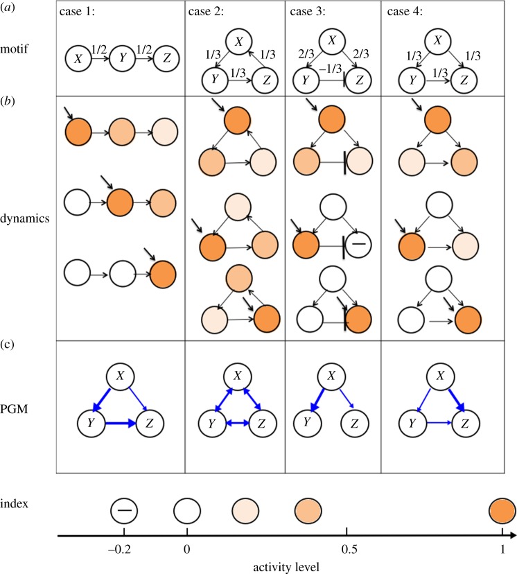
In the case of three units, there are several ways to connect them. We choose four distinct connectivity configurations that provide distinct functionality, shown in figure 4a. The configurations are: (i) A simple chain from X to Y to Z, with weights ; (ii) A simple loop, with weights ; (iii) Inhibition edge from Y to Z, with weight , ; (iv) Three edges that constitute a directed acyclic network, with weights . All other unassigned weights are 0. We call these static connectivity maps connectomes. Our goal is to infer functional connectivity based on the connectome and the network dynamics.

Figure 4.

Construction of PGMs for three-unit motifs. (a) Connectomes of four examined motifs. (b) Network responses when external input is injected into each unit (indicated by diagonal arrow). The colour of the units indicate the activation level of each unit, i.e. darker colour indicates a more active node. (c) Constructed PGM structures. If there is an edge from X to Y, then the conditional probability P(Y | X) > 0.1. Stronger arrows correspond to higher probability.

To simulate the dynamics, we inject a constant input of 1 unit into a specific neuron and record network response in a snapshot matrix. We then apply SVD on the snapshot matrix and extract the dominant modes, as described in the previous section. For example, in case 2, the network is simulated for a sufficiently long time with stimuli {I₁, I₂, I₃} set to {[1, 0, 0], [0, 1, 0], [0, 0, 1]} independently. Applying the method yields the pairwise dependency matrix P

The elements of P are used as approximations to conditional probabilities:

If we add Gaussian noise to the simulation, we obtain a slightly perturbed pairwise dependency matrix P̃:

which demonstrates that the SVD-based approach is robust to noise.

Owing to the simplicity of the motifs, we can validate the PGM via an analytical dynamical systems approach by calculating the fixed points. For case 2, the fixed point induced by input into node X is (u*₁, u*₂, u*₃) ≈ (1, 0.2507, 0.0817), which is exactly the value of the conditional probabilities we computed using the PGM construction approach. Because all edge weights are identical, the same fixed point will be induced by input into the other two nodes up to shuffling of the indices.

We also calculate the correlation coefficients directly from the time series, and obtain a correlation matrix Q:

With the same Gaussian noise added to the system, the correlation matrix is greatly perturbed, resulting in a matrix Q̃:

Notably, the matrix Q̃ does not represent the functional connectivity of the underlying system; particularly note the negative correlation between X and Y . In addition, the matrices Q and Q̃ are substantially different, indicating the sensitivity of the correlation approach to noise. In summary, these examples demonstrate that our proposed SVD approach is more appropriate to capture the intrinsic dynamics and statistical dependency between nodes.

A similar validation process can be used for other configurations. We include their analysis in the Appendix. To infer the functional connectivity graph, we apply the RID algorithm to the dependency matrix P and set the threshold to be 0.1 and the maximum depth of the tree as 3, because there are only three nodes. Three individual trees are constructed for each case. Combination of them into one graph is shown in figure 4c. Comparing figure 4a (connectome) with 4c (PGM), we observe that the PGMs have different structures from their corresponding connectomes. Indeed, the edges in the PGM represent the conditional dependencies instead of weights and reflect how the motif processes inputs. In particular, in case 1 the PGM shows that Y strongly depends on X, and Z strongly depends on Y, which corresponds to the chain structure of the motif. It also demonstrates weaker dependence of Z on X, which is not trivially seen in the connectome. In case 2, the PGM indicates symmetry and interdependence between all the nodes. Thereby input injection into any node will produce an equivalent response, a characteristic of a circular structure of the motif in this case. Notably, the motif's connectome shows propagation in one direction, while the PGM estimates symmetric behaviour. In case 3, there is an inhibitory edge between Y and Z, resulting in a negative dependence, and we consider two approaches here: one is to set the conditional probability to zero and eliminate the edge between Y and Z in the functional connectome (as shown in figure 4). Another way is to take the absolute value of the dominant modes (as described in algorithm 1), and show a positive dependence from Y to Z. The first approach ignores the negative causality: while the second approach retains some information of the causality; therefore we adopt the second approach in the C. elegans study described below. Also, even though the weights w_XY and w_XZ are the same in the connectome, the dependency from Y to X in the PGM is stronger than the dependency from Z to X. Such an effect is due to inhibition of stimulus propagation from X to Z through Y. In comparison, in case 4, where the inhibitory edge between Y and Z is replaced by an excitatory edge, the PGM indicates that Y enhances the propagation of stimulus from X to Z, even though the weights w_XY and w_XZ are all identical. These exemplary cases demonstrate that PGM structure is different from the motif's connectome and captures the functional dependencies between the nodes. These dependencies are not trivial to conclude from the connectome structure alone and become more complex as the dimension of the motif and ratio of connections change.

4. Application to neurobiological dynamic connectome

(a). Neuronal network of Caenorhabditis elegans

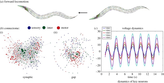
The nematode Caenorhabditis elegans nervous system is a well-studied system, consisting of 302 neurons identifiable and consistent across individuals. The connections between the neurons are composed of chemical synapses and gap junctions, whose wiring diagrams, i.e. connectomes, are nearly fully resolved from serial section electron microscopy [14]. In addition to the connectomes, the dynamic model that describes the biophysical processes between neurons has been introduced [20]. Specifically, the dynamical model of the nervous system is governed by a system of nonlinear differential equations (figure 5):

where C is the whole-cell membrane capacitance, G^c is the membrane leakage conductance and E_cell is the leakage potential. I^Ext_i is the external input current injected to the ith neuron. I^Gap_i and I^Syn_i correspond to the input currents modelling gap junctions and synapses, respectively. More details on the biophysical model can be found in [20] and in the Appendix.

Figure 5.

Two layers of the neuronal network of C. elegans. (a) An example of forward locomotion induced by two layers of the neuronal network of the worm (image credit http://www.connectomeengine.com/). The first layer (b): connectome of C. elegans, consisting of 297 somatic neurons, 6393 chemical synapses and 890 gap junctions. The connectome shows (i) the chemical synapses between neurons and (ii) the gap junctions. The second layer (c): neural dynamics modelled by differential equations. Here, we show voltage oscillations of the motor VB group. Combining the two layers we achieve the dynome, a dynamically evolving network, which is the foundation for constructing the PGM.

Combining the connectome and the dynamical model constitute the dynome of C. elegans. Incorporating both the layers of connectivity and dynamic biophysical processes, the C. elegans dynome models the nervous system functionality and processing of stimuli that it performs. Indeed, when provided with arbitrary input stimuli, the C. elegans dynome is capable of producing various forms of characteristic dynamics such as static, oscillatory, non-oscillatory and transient voltage patterns consistent with experimentally observed ones [20,26]. These simulated dynamics indicate that the C. elegans dynome is a valuable model for the worm's nervous system and thus a suitable foundation for the construction of its probabilistic graphical model.

(b). Constructing dependencies

We apply our method to the neuronal network of the C. elegans nematode by injecting scaled input current into each of the n = 279 neurons independently using the Neural Interactome platform (see [21,27] for further details). We run the simulations for 15 s with a time step of 0.01 s and record the dynamics of all neurons in snapshot matrices with each snapshot matrix S of dimensions n × T = 279 × 1501. We then subtract the activation threshold for each neuron from the simulation and exclude the initialization phase of the network (1 s). We then obtain 279 response vector representations of all neurons to the stimulation of the input neurons by performing SVD on each snapshot matrix and taking the weighted sum of all modes as described in §2. Each of these vectors is normalized according to input neuron response, which yields the conditional probability P(X_j = 1 | X_i = 1) as elements of the vector. The vectors are stored as column vectors of the conditional probability table, resulting in a 279 × 279 dependency matrix, which records the complete pairwise dependencies of the nodes in the C. elegans neuronal network.

5. Caenorhabditis elegans functional connectome represented by probabilistic graphical model

(a). Anatomical connectomes compared with probabilistic graphical model functional connectome

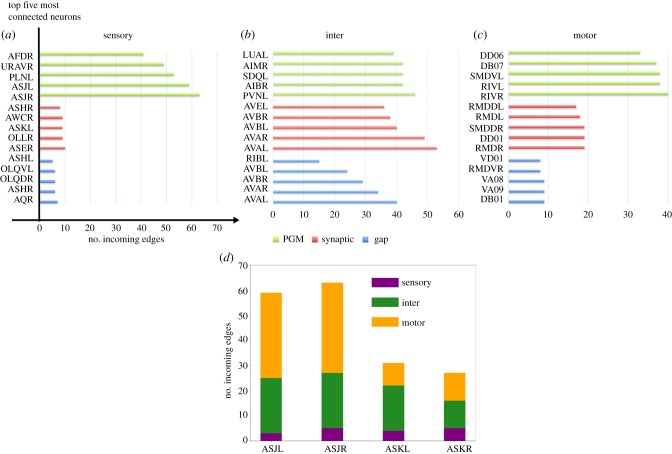
We compare the dependency matrices (functional connectome) obtained from our PGM construction with the anatomical (gap and chemical connectomes) in figures 6 and 7. Figure 6 compares top connected (hub) neurons in each group type (sensory, inter and motor) across the three different connectomes. The definition of connectivity for synaptic and gap connectomes is straightforward and we use the number of incoming edges as a count for connectivity. The connectivity in the PGM is expressed through probabilistic interaction and thereby top connected neurons are the neurons with the highest conditional probability. Notably, the PGM identifies a vastly different set of hub neurons compared with those identified by synaptic and gap connectomes. In particular, we observe that ‘hub’ neurons in the synaptic and gap connectomes, such as AVA and AVB, are not listed in PGM's top connected neurons. Furthermore, top sensory and motor neurons in PGM receive far more connections than neurons from the same group in the synaptic and gap connectomes.

Figure 6.

Top connected neurons in sensory, inter and motor groups. (a–c) We compare three groups: functional connectivity represented by PGM, connectome mapping chemical synapses, and a connectome mapping gap junction. Connectivity is measured by the number of incoming edges. Top five connected neurons in each group along with the number of incoming edges into them are shown. In the synaptic group, an edge exists from one node (X_i) to another (X_j) if there is at least one chemical synapse X_i → X_j. In the gap group, an edge exists between X_i and X_j when there is at least one gap junction between X_i and X_j, as the gap junctions are non-directed. In the PGM group, an edge exists from X_i to X_j if P(Y = 1|X = 1) > threshold, set here as threshold = 0.1. (d) Number of incoming edges in the PGM for ASJ and ASK sensory neurons, categorized into three classes (sensory, inter and motor).

Figure 7.

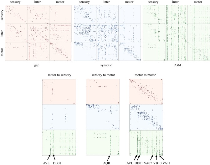
Connectivity matrices of gap, synaptic and PGM. In the dependency matrices, the element in the jth column and ith row, a_ji, represents the total number of gap contacts/synaptic contacts, probability dependencies respectively from ith neuron to jth neuron. The subplots motor sensory, motor motor, sensory motor are zoomed in to compare detailed differences in gap, synaptic and PGM connections. Input neurons that activate the majority of the responding neurons are labelled.

From sensory neurons, PGM highlights ASJ, PLNL, URAVR and AFDR as the neurons with the most probabilistic interactions. These neurons are reported to be associated with avoidance behaviours under different circumstances in the environment. ASJ neurons take part in light sensation and promote reversals [28] while PLN neurons are part of the sensory group associated with oxygen sensing [29]. URA neurons are generally considered as sensory neurons but also innervate head muscles via the nerve ring [30]. AFD neurons are considered as thermo-sensors and promote turns on encounters with high temperature [31]. It is particularly intriguing to find ASJ neurons as top functional neurons, as they are anatomically sparsely connected sensory neurons. We investigated the reason for such discrepancy by looking at the incoming neurons related to ASJ and comparing them with ASK neurons, which have the reverse property: they are anatomically well connected neurons but not functionally (figure 6d). Our comparison shows that the majority of incoming edges (60%) into ASJ in the PGM are motor neurons, whereas for ASK, despite being connected to ASJ, there are significantly fewer functional interactions with motor neurons and consequently a smaller number of incoming edges. These results suggest that ASJ may have substantial interactions with motor neurons and possibly a particular role in motor coordination, e.g. proprioceptive feedback, where motor neurons interact with sensory neurons. Further analysing the PGM, we discovered that the AVA, DB01, PVC, VA motor group and DVC neurons have the highest probabilities of triggering ASJ neurons. As many of these neurons are associated with backward locomotion, one can speculate that, despite its low connectivity, ASJ could be more widely implicated in reversal and avoidance behaviours than previously known in the literature. Similar observation can be made with respect to PLNL, URAVR and AFDR. These neurons are not particularly well connected in the anatomical connectomes, but have a high number of probabilistic interactions with neurons associated with backward motion.

Inter neurons associated with avoidance and locomotion appear to be functionally dominating. PGM identifies LUA, PVN, SDQ, AIM, AIB neurons as the top connected ones. While the exact functions of LUA and PVN are not very well known, LUA is suggested to function as a connector cell between PLM touch receptors and ventral cord, suggesting its potential role in locomotion [32]. While AIM neurons are speculated to modulate the locomotion circuit via regulating extra-synaptic serotonin [33], SDQ and AIB neurons, on the other hand, are known to be associated with high oxygen avoidance and promotion of turn, respectively [29].

As in other groups, within the motor neurons group we find that the top connected neurons are associated with turning/locomotion behaviours. Both RIV and SMD neurons innervate neck/head muscles that modulate avoidance/escape behaviours such as omega turns [34], and both DD06 and DB07 neurons are components of main modulators controlling turns and locomotion, respectively, in the dorsal cord upon their activation [35]. Furthermore, we observe that the majority of the neurons that have probabilistic interactions with DD06 and DB07 in the PGM are members of body wall motor neurons such as the A, B and AS groups. The results suggest that DD06 and DB07 may serve as hub neurons within the array of motor neurons distributed throughout the worm's body wall. Indeed, some studies propose repeated network motifs within the body wall motorneuronal connectivity as a mechanism that facilitates locomotion [36]. Taken together, our results provide new insights into the worm's neural function by (i) suggesting the importance of avoidance/turning behaviours to the organism, and (ii) suggesting the potential functional importance of neurons whose roles are currently unclear.

In figure 7, we visualize side-by-side the PGM dependency matrix and the anatomical connectomes with the direction of the connectivity being (from,  to) and the neurons are ordered by location (anterior to posterior), similar to the order in [14]. This visualization shows the unique characteristics of each connectome. Gap connections appear to be mostly local, i.e. clustered around the diagonal, in which physically neighbouring neurons have gap junctions. Also there are a few horizontal and vertical ‘chains’ in inter and motor neurons, which correspond to single neurons having gap junctions with multiple neurons. Synaptic connections incorporate dense connectivity patterns (inter–inter, sensory but not functionally inter) in addition to local structure and a few connectivity chains. Furthermore, sensory inter and inter motor connections are well established in the anatomical connectomes, while sensory motor connections are rarer.

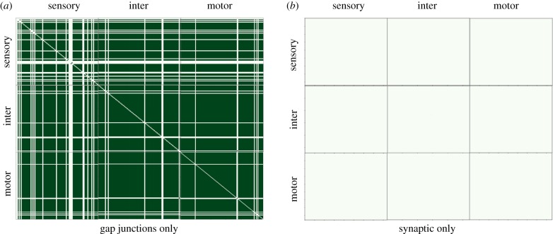
PGM connectivity appears to be structured differently from the anatomical connectomes, with local responses being less profound. Most of the dominant patterns appear to be vertical chains. Each chain corresponds to a receiving neuron triggered by stimulation of multiple neurons across groups. Triggering neurons are also distant neurons with no gap or synaptic connections. Most of the vertical chains appear in inter and motor neuron groups. In addition, we observe that excitation of sensory neurons leads to excitation of motor neurons, and motor neurons in reverse also impact sensory neurons. Such observations could be related to the known ability of sensory neurons to trigger motor behaviours and motor neurons to influence sensation. Another observation from PGM visualization is that there are no dominant horizontal chains indicating that a single neuron response is triggered by only a few input neurons. To understand how each anatomical connectome contributes to the PGM structure we constructed PGMs by including only a single anatomical connectome (gap or synaptic) in the neural dynamics simulator (see figure 10). The PGM associated with the synaptic-only dynamical model results in a graph with extremely sparse dependencies, indicating that only trivial dynamics persist. In particular, we do not observe outgoing edges from ALML/R, PLML/R known to be functional in locomotion behaviour. On the other hand, the PGM constructed from the gap-only dynamical model turned out to be extremely dense, with many distinct and additional functional connections not present in the PGM constructed from the full dynamical model. For example, for the ALML/R PLML/R neurons, we note that a different set of motor neurons is activated. These experiments indicate that both anatomical connectomes are required to produce adequate neural dynamics. In terms of contribution to the PGM construction, we observe that the synaptic connectome serves as a selective filter to gap-only functional connections.

Figure 10.

PGM dependency matrices constructed by including a single anatomical connectome (a: gap; b: synaptic) in the neural dynamics simulator. (Online version in colour.)

(b). Inference of functional sub-circuits

While global features of functional properties could be obtained through visualizing the PGM dependency matrix, additional analysis is needed to retrieve specific features such as pathways of neural information flow from a neuron of interest or a cluster of neurons. Such pathways can be inferred through posterior inference traversing the PGM. We pose two types of inference queries on the pairwise conditional table. (i) Given a set of input neurons: What is the set of downstream neurons most likely to be activated? For example, such inference is relevant to identify inter and motor neurons activated by a set of sensory neurons. (ii) Given a set of downstream neurons: What are the subsets of upstream and midstream neurons most likely to activate these downstream neurons? Such inference can reveal, for example, inter neurons and sensory neurons that are most probably to activate motor neurons. Both of these questions can be answered by constructing a graphical model for the network and performing posterior inference. While the first problem follows stimulus propagation forward, the second problem is an inverse problem, often called the MAP problem, and requires examination and optimization over many probable inverse propagation sequences. We summarize our key results below and include individual neuron trees in the Appendix.

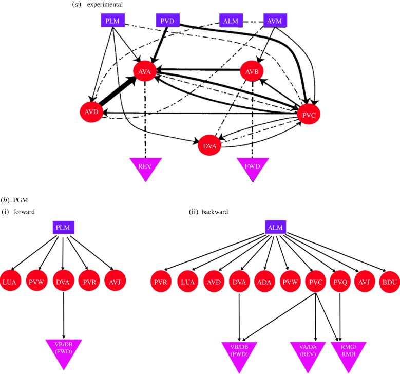
To infer downstream neurons, we start with a set of input nodes and use the RID algorithm to construct a response tree for each input node in the set. For each parent node, we explore all of its children that have conditional dependency exceeding 0.1 in descending order. For simplicity, we restrict the tree to having a maximum depth of 3—one layer each of sensory, inter and motor neurons—to keep the flow from sensory to motor neurons straightforward. In particular, we focus on well-known experimental scenarios such as forward and backward locomotion, as shown in figure 8. Specifically, we investigate forward locomotion triggered by posterior touch: activation of sensory PLML/R neurons results in the activation of the DB and VB groups, associated with forward locomotion. We investigate this sub-circuit by constructing a tree with input nodes PLML and PLMR (labelled PLM). Both neurons activate the same set of inter neurons, LUA, PVR, PVW, AVJ, DVA, i.e. these neurons have the highest probabilities conditioned on the activation of PLML and PLMR sensory neurons and lead to motor neurons. Other inter neurons do not lead to any immediate motor neurons. The DVA neuron leads to the DB01 motor neuron in group B (motor neurons group associated with forward movement [32]), which in turn activates most of the motor neurons in the DB and VB groups. These results are consistent with functional stimulus propagation flow reported in the literature.

Figure 8.

Sub-circuits that lead to forward and backward locomotion in C. elegans (a) Experimentally proposed connectome sub-circuit of forward and backward locomotion (sensory neurons are shown by rectangles, inter neurons by circles and motor neurons by triangles: FWD, forward; REV, reverse). Lines with arrows refer to chemical synapses and dashed lines refer to gap junctions. Reproduced from [18]. (b) Sub-circuits inferred from PGM. (i) Forward locomotion induced by injecting input into sensory neurons PLML and PLMR, known to trigger forward locomotion upon posterior touch. (ii) Backward locomotion induced by injecting input into ALML and ALMR, known to trigger backward locomotion upon anterior touch. (Online version in colour.)

We also examine anterior touch, triggered by stimulation of ALML and ALMR (labelled ALM) neurons, which leads to backward locomotion. ALM activation leads to a larger set of inter neurons. The set contains all inter neurons associated with forward locomotion and additionally includes AVD, ADA, PVC, PVQ and BDU, most of which are indeed associated with backward movement. Indeed, AVD is experimentally known to be associated with backward locomotion, and PVC plays an important role in both forward and backward motion [18,30]. Stimulus flows from the PVC neuron to several motor neurons, especially neurons in group A, i.e. DA, VA (experimentally identified as associated with backward movement), as well as in DB and VB groups.

Compared with the circuit extracted from the synaptic and gap connectomes in figure 8a from [18], the PGM successfully recovers neurons participating in this circuit and separates them into two functional sub-circuits. In each of the sub-circuits, motor neurons are reached to induce locomotion. As can be seen from the circuit sketch, separation into independent circuits is nontrivial. The PGM also identifies inter neurons such as AVD, PVC and DVA, while the hub neurons AVA and AVB are missing. A possible explanation is that individual activation of ALM or PLM is insufficient for AVA/AVB to reach a strong state of excitation and they are activated through another stimulation/process.

We use MAP inference to perform reverse tracking of activating neurons of motor neurons associated with locomotion. We, thus, choose motor neurons in the ventral cord members of A and B groups shown as triangles in figure 9 and labelled as DA, VA, DB, VB, DD, VD. Posterior MAP inference finds inter and sensory neurons, which are most likely to activate the given motor neurons. Specifically, we apply the RID algorithm and flipped conditional probabilities. Instead of sorting P(X_i | X_j), we sort P(X_j | X_i), with X_j being the parent node. As in forward RID, we limit the depth of the tree to be 3 and keep one layer each of motor, inter and sensory neurons. We find ten inter neurons and six sensory neurons that most frequently appear in the reverse traversal paths. We list these neurons in figure 9 as circles (inter) and rectangles (sensory). Notably, most of sensory and inter neurons that MAP inference produces were indeed experimentally associated with locomotion, and these are neurons that we identified in PLM and ALM pathways in figure 8. Furthermore, additional neurons known to participate in locomotion are identified. Inferred inter neurons now do include AVA and AVB, which were not present in forward inference from ALM and PLM (see figure 8), emphasizing that when additional paths are considered, these neurons do play a role in sensory–motor neural integration, but not in direct stimulation of ALM and PLM. The power of MAP inference is in its ability to associate additional neurons with the designated motor neurons, without any prior biological knowledge of the network. For example, additional inferred sensory neurons include AQR and PQR, known experimentally to influence locomotion. Their function is currently being studied and conjectured to be associated with oxygen sensation and avoidance [37]. Using MAP inference in PGM we, thereby, are able to support this conjecture. The posterior inference from these neurons would provide more detail about which pathways the stimulus from AQR and PQR is following to reach locomotion motor neurons.

Figure 9.

MAP posterior inference: reverse tracking of A and B motor groups associated with locomotion. We identify a group of neurons using MAP inference. Given that a specific group of motor neurons are being excited, the set of inter and sensory neurons that leads to such excitation is shown. From top to bottom is the natural stimulus flow, i.e. sensory → inter → motor. From bottom to top is MAP inference. (Online version in colour.)

6. Discussion

We presented a new approach to forming a graphical model (PGM) for a neuronal network. Two key components in our approach allow us to construct the PGM that captures network functionality. The first component is the underlying dimension reduction technique to obtain a low-dimensional projection of network responses to stimuli. The second component is that we capture network responses to independent stimuli (single neuron stimulation). We thus consider pairwise dependencies instead of full dependencies on the whole network and greatly reduce the number of parameters. This constraint-based approach is computationally efficient and allows posterior inference when combined with a method for traversing the PGM to produce response trees (RID).

We describe how to apply these techniques to simple motif examples and to a neuronal model of the C. elegans nervous system whose anatomical connectomes and dynamics have been resolved. The application to C. elegans neuronal activity identified key neurons and sub-circuits without any prior knowledge of their functionality. In particular, our findings prompt additional examination of functional roles for some of the neurons outlined by PGM. Ultimately, determination and validation of the roles of these neurons should be performed in experimental settings or by coupling neural dynamics with biomechanical models of muscles and body. Furthermore, the constructed PGM can be used for extraction of additional pathways associated with stimuli and behaviours that we did not consider here. Notably, the pathways inferred using the PGM indicate that if a particular neuron is excited electrophysiologically or optogenetically, the neurons included in the associated pathway tree will be most responsive to this excitation. While we applied the methodology to construct the PGM from simulation-driven data, a similar approach could be implemented in an experimental setting using single-neuron clamping and multi-neuron imaging network dynamics. Likewise, the methodology introduced here can be applied to other network models and organisms.

Our framework assumes that the underlying network structure remains isotropic over simulation time, that is, the anatomical connectomes and pairwise conditional probabilities P(B|A) remain similar if the simulation is continued for a longer time, unlike networks that undergo rewiring during simulation time, studied in previous works [5,6]. From a dynamical point of view, we expect our approach to perform best when the simulated network dynamics converge to low-dimensional attractors. Indeed, for the C. elegans network, stimuli-induced low-dimensional attractors were shown to exist in the network and simulation of the network for an efficiently long period (15 s) is expected to capture attractor dynamics [20].

The dimension reduction employed here is based on SVD. We collapse all SVD modes into a single vector by computing a weighted sum according to singular values of all modes. A plausible reduction is to retain the modes composing 90% or more of the total energy. In many simulations of C. elegans, the first two modes indeed take up more than 90% of the energy and the first four modes take up more than 99%. This is consistent with the observation that behavioural manoeuvres are spanned by several modes [38]. Indeed, we observe only a minor difference between taking the weighted sum of all modes and with taking the weighted sum of the first two modes. As expected, we do see a significant difference between using the weighted sum of the first two modes and just the dominant mode, indicating that attractors are spanned by at least a two-dimensional space. Notably, it is also possible to use other approaches to compress the modes into a single vector, for example, a combination of k-rank approximation with methods such as Exclusive Threshold Reduction and Optimal Exclusive Threshold Reduction, introduced in [39].

By independent stimulation and activation of each neuron followed by construction of pairwise response probabilities, our approach assumes that responses could be superimposed, i.e. the response probability caused by two or more stimuli is the sum of the responses that would have been caused by each stimulus individually. While, in general, the assumption is not guaranteed to hold in nonlinear neuronal systems, networks that have input induced attractors, such as the C. elegans system and other attractor systems where there are many functionalities, are an aggregate of response patterns to individual stimulations. Theoretically, it is possible to construct a Bayesian network D(G, θ) with θ_i = P(X_i | X₁, …, X_n), in which we go beyond the pairwise conditional probabilities and explore all the possible assignments to all the variables in the set. Specifically, we either activate each node in the network, or force it to be inactive. However, doing so requires us to specify 2ⁿ distributions and would require much more simulations such that for large n the construction will become computationally intractable.

Our approach for measuring probabilistic dependencies in dynamic processes is different from previously introduced approaches. Alternative approaches propose constructions which are based on measuring correlations or causality that collapse time and can possibly lose valuable information. In this realm, another possibility is to consider time-dependent PGMs. However, the posterior inference becomes ill-defined and inefficient as for the original dynamical model from which the PGM is constructed. Our approach is therefore considered as a hybrid of the two aforementioned approaches because it uses spatio-temporal dimension reduction with pairwise probabilities constraint to produce a static PGM for which posterior inference is fast and well defined.

The posterior inference could also be performed in real time, by incorporating simulations as the inference occurs, i.e. simulate the network and construct probabilities from time-series snapshot matrices. Such an extension will allow us to relax the pairwise probabilities constraint and potentially lead to the more accurate representation of information flow. We did not choose such an approach because it is time-consuming and requires performing network simulations for every inference task. In practice, for a network with more than a few nodes, real-time inference becomes intractable. We thereby pre-process network responses as pairwise dependencies and construct a pre-processed PGM for which inference is a standard procedure in a statistical model.

Appendix

(a) Analytical validation of motif examples

For case 1, a simple chain, we set the weights , , and all other weights to be zero. Then the network dynamics are as follows:

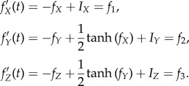1. Fixed point:

   
2. Linearization:

   

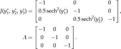
As all eigenvalues are negative real numbers, the system is stable at the fixed point.

Using algorithm 1, the conditional probabilities obtained from simulated data are as follows:

which is consistent with the analytical results. If we add Gaussian noise to the system, we get approximately the same result, which validates that our approach is robust to noise.

For case 3 with feedforward inhibition, suppose , , , and all others are zero. Then the network dynamics are as follows:

1. Fixed point:

   
2. Linearization:

   

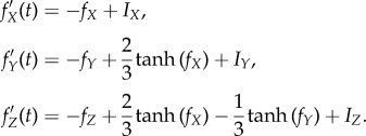As all eigenvalues are negative real numbers, the fixed point is stable.

Using algorithm 1, the conditional probabilities obtained are as follows:

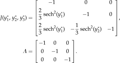
For case 4 with feedforward excitation, suppose , , , and all others are zero. Then the network dynamics are as follows:

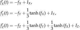1. Fixed point:

   
2. Linearization:

   

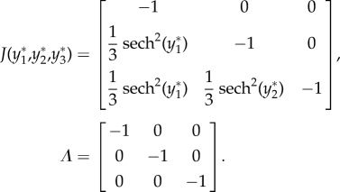
As all eigenvalues are negative real numbers, the fixed point is stable.

Using algorithm 1, the conditional probabilities obtained are as follows:

(b) Caenorhabditis elegans dynamics

The dynamic model of the neuronal network is governed by a system of nonlinear differential equations:

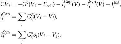where G^g_ij is the total conductivity of the gap junctions between i and j, and G^s_ij is the maximum total conductivity of synapses from j to i. The synaptic activity variable, s_i, is governed by

where a_r and a_d correspond to the synaptic activity's rise and decay time s, V_th is voltage at equilibrium, and ϕ is the sigmoid function with width β:

Data accessibility

To simulate C. elegans neural dynamics we use the Neural Interactome available at [21,27] and store the dynamics as Python matrices. Python software to construct the PGM for C. elegans is available at [40].

Competing interests

We declare we have no competing interests.

Funding

The work was supported by the National Science Foundation under grant nos DMS-1361145, the Air Force Office of Sponsored Research under grant no. FA95501610167, and the Washington Research Foundation Innovation Fund. The authors would also like to acknowledge the partial support by the Departments of Applied Mathematics, and Electrical Engineering at the University of Washington.

References

- 1.Koller D, Friedman N, Getoor L, Taskar B. 2007. Graphical models in a nutshell. In Introduction to statistical relational learning, pp. 13–55. Cambridge, MA: MIT press. [Google Scholar]
- 2.Koller D, Friedman N. 2009. Probabilistic graphical models: principles and techniques. Cambridge, MA: MIT Press. [Google Scholar]
- 3.Murphy KP. 2012. Machine learning: a probabilistic perspective. Cambridge, MA: MIT Press. [Google Scholar]
- 4.Friedman N, Linial M, Nachman I, Pe'er D. 2000. Using Bayesian networks to analyze expression data. J. Comput. Biol. 7, 601–620. ( 10.1089/106652700750050961) [DOI] [PubMed] [Google Scholar]
- 5.Kolar M, Song L, Ahmed A, Xing EP. 2010. Estimating time-varying networks. Ann. Appl. Stat. 4, 94–123. ( 10.1214/09-aoas308) [DOI] [Google Scholar]
- 6.Ahmed A, Xing EP. 2009. Recovering time-varying networks of dependencies in social and biological studies. Proc. Natl Acad. Sci. USA 106, 11 878–11 883. ( 10.1073/pnas.0901910106) [DOI] [PMC free article] [PubMed] [Google Scholar]
- 7.Honey CJ, Kötter R, Breakspear M, Sporns O. 2007. Network structure of cerebral cortex shapes functional connectivity on multiple time scales. Proc. Natl Acad. Sci. USA 104, 10 240–10 245. ( 10.1073/pnas.0701519104) [DOI] [PMC free article] [PubMed] [Google Scholar]
- 8.Butte AJ, Kohane IS. 2000. Mutual information relevance networks: functional genomic clustering using pairwise entropy measurements. In Pacific Symp. Biocomputing 2000 (ed. Altman RB, Dunker AK, Hunter L, Lauderdale K, Klein TE), pp. 418–429. Singapore: World Scientific. [DOI] [PubMed] [Google Scholar]
- 9.Basso K, Margolin AA, Stolovitzky G, Klein U, Dalla-Favera R, Califano A. 2005. Reverse engineering of regulatory networks in human B cells. Nat. Genet. 37, 382–390. ( 10.1038/ng1532) [DOI] [PubMed] [Google Scholar]
- 10.Zhang L, Guindani M, Vannucci M. 2015. Bayesian models for functional magnetic resonance imaging data analysis. Wiley Interdiscip. Rev. Comput. Stat. 7, 21–41. ( 10.1002/wics.1339) [DOI] [PMC free article] [PubMed] [Google Scholar]
- 11.Zhang J. et al. 2014. Inferring functional interaction and transition patterns via dynamic Bayesian variable partition models. Hum. Brain Mapp. 35, 3314–3331. ( 10.1002/hbm.22404) [DOI] [PMC free article] [PubMed] [Google Scholar]
- 12.Ozdemir A, Bernat EM, Aviyente S. 2017. Recursive tensor subspace tracking for dynamic brain network analysis. IEEE Trans. Signal Inf. Process. Networks 3, 669–682. ( 10.1109/TSIPN.2017.2668146) [DOI] [Google Scholar]
- 13.Yizhar O, Fenno LE, Davidson TJ, Mogri M, Deisseroth K. 2011. Optogenetics in neural systems. Neuron 71, 9–34. ( 10.1016/j.neuron.2011.06.004) [DOI] [PubMed] [Google Scholar]
- 14.Varshney LR, Chen BL, Paniagua E, Hall DH, Chklovskii DB. 2011. Structural properties of the Caenorhabditis elegans neuronal network. PLoS Comput. Biol. 7, e1001066 ( 10.1371/journal.pcbi.1001066) [DOI] [PMC free article] [PubMed] [Google Scholar]
- 15.Goodman MB, Hall DH, Avery L, Lockery SR. 1998. Active currents regulate sensitivity and dynamic range in C. elegans neurons. Neuron 20, 763–772. ( 10.1016/S0896-6273(00)81014-4) [DOI] [PMC free article] [PubMed] [Google Scholar]
- 16.Kato S, Kaplan HS, Schrödel T, Skora S, Lindsay TH, Yemini E, Lockery S, Zimmer M. 2015. Global brain dynamics embed the motor command sequence of Caenorhabditis elegans. Cell 163, 656–669. ( 10.1016/j.cell.2015.09.034) [DOI] [PubMed] [Google Scholar]
- 17.Nguyen JP, Shipley FB, Linder AN, Plummer GS, Liu M, Setru SU, Shaevitz JW, Leifer AM. 2016. Whole-brain calcium imaging with cellular resolution in freely behaving Caenorhabditis elegans. Proc. Natl Acad. Sci. USA 113, E1074–E1081. ( 10.1073/pnas.1507110112) [DOI] [PMC free article] [PubMed] [Google Scholar]
- 18.Wicks SR, Roehrig CJ, Rankin CH. 1996. A dynamic network simulation of the nematode tap withdrawal circuit: predictions concerning synaptic function using behavioral criteria. J. Neurosci. 16, 4017–4031. ( 10.1523/JNEUROSCI.16-12-04017.1996) [DOI] [PMC free article] [PubMed] [Google Scholar]
- 19.Shlizerman E, Schroder K, Kutz JN. 2012. Neural activity measures and their dynamics. SIAM J. Appl. Math. 72, 1260–1291. ( 10.1137/110843630) [DOI] [Google Scholar]
- 20.Kunert J, Shlizerman E, Kutz JN. 2014. Low-dimensional functionality of complex network dynamics: neurosensory integration in the Caenorhabditis elegans connectome. Phys. Rev. E 89, 052805 ( 10.1103/PhysRevE.89.052805) [DOI] [PubMed] [Google Scholar]
- 21.Kim J, Leahy W, Shlizerman E. 2017. Neural Interactome: interactive simulation of a neuronal system bioRχiv, 209155 ( 10.1101/209155) [DOI] [PMC free article] [PubMed]
- 22.Stewart GW. 1991. Perturbation theory for the singular value decomposition. In SVD and signal processing II: algorithms analysis and applications (ed. Vacarro RJ.), pp. 99–109. Amsterdam: Elsevier. [Google Scholar]
- 23.Shlizerman E, Schroder K, Kutz JN. 2012. Neural activity measures and their dynamics. SIAM J. Appl. Math. 72, 1260–1291. ( 10.1137/110843630) [DOI] [Google Scholar]
- 24.Friedman J, Hastie T, Tibshirani R. 2001. The elements of statistical learning (Springer Series in Statistics, vol. 1). New York: Springer. [Google Scholar]
- 25.Funahashi K-I, Nakamura Y. 1993. Approximation of dynamical systems by continuous time recurrent neural networks. Neural Networks 6, 801–806. ( 10.1016/S0893-6080(05)80125-X) [DOI] [Google Scholar]
- 26.Kunert-Graf JM, Shlizerman E, Walker A, Kutz JN. 2017. Multistability and long-timescale transients encoded by network structure in a model of C. elegans connectome dynamics. Front. Comput. Neurosci. 11, 53 ( 10.3389/fncom.2017.00053) [DOI] [PMC free article] [PubMed] [Google Scholar]
- 27.Kim J. 2018. C. elegans Neural Interactome β See https://github.com/shlizee/C-elegans-Neural-Interactome.
- 28.Ward A, Liu J, Feng Z, Xu XS. 2008. Light-sensitive neurons and channels mediate phototaxis in C. elegans. Nat. Neurosci. 11, 916–922. ( 10.1038/nn.2155) [DOI] [PMC free article] [PubMed] [Google Scholar]
- 29.Zimmer M. et al. 2009. Neurons detect increases and decreases in oxygen levels using distinct guanylate cyclases. Neuron 61, 865–879. ( 10.1016/j.neuron.2009.02.013) [DOI] [PMC free article] [PubMed] [Google Scholar]
- 30.Altun Z, Hall D. 2002. WormAtlas. See http://www.wormatlas.org, vol. 1384. [Google Scholar]
- 31.Mori I, Ohshima Y. 1995. Neural regulation of thermotaxis in Caenorhabditis elegans. Nature 376, 344–348. ( 10.1038/376344a0) [DOI] [PubMed] [Google Scholar]
- 32.Chalfie M, Sulston JE, White JG, Southgate E, Thomson JN, Brenner S. 1985. The neural circuit for touch sensitivity in Caenorhabditis elegans. J. Neurosci. 5, 956–964. ( 10.1523/JNEUROSCI.05-04-00956.1985) [DOI] [PMC free article] [PubMed] [Google Scholar]
- 33.Jafari G, Xie Y, Kullyev A, Liang B, Sze JY. 2011. Regulation of extrasynaptic 5-HT by serotonin reuptake transporter function in 5-HT-absorbing neurons underscores adaptation behavior in Caenorhabditis elegans. J. Neurosci. 31, 8948–8957. ( 10.1523/JNEUROSCI.1692-11.2011) [DOI] [PMC free article] [PubMed] [Google Scholar]
- 34.Gray JM, Hill JJ, Bargmann CI. 2005. A circuit for navigation in Caenorhabditis elegans. Proc. Natl Acad. Sci. USA 102, 3184–3191. ( 10.1073/pnas.0409009101) [DOI] [PMC free article] [PubMed] [Google Scholar]
- 35.Donnelly JL, Clark CM, Leifer AM, Pirri JK, Haburcak M, Francis MM, Samuel AD, Alkema MJ. 2013. Monoaminergic orchestration of motor programs in a complex C. elegans behavior. PLoS Biol. 11, e1001529 ( 10.1371/journal.pbio.1001529) [DOI] [PMC free article] [PubMed] [Google Scholar]
- 36.Haspel G, O'Donovan MJ. 2012. A connectivity model for the locomotor network of Caenorhabditis elegans. In Worm, vol. 1, pp. 125–128. London: Taylor & Francis; ( 10.4161/worm.19392) [DOI] [PMC free article] [PubMed] [Google Scholar]
- 37.Chang AJ, Chronis N, Karow DS, Marletta MA, Bargmann CI. 2006. A distributed chemosensory circuit for oxygen preference in C. elegans. PLoS Biol. 4, e274 ( 10.1371/journal.pbio.0040274) [DOI] [PMC free article] [PubMed] [Google Scholar]
- 38.Stephens GJ, Johnson-Kerner B, Bialek W, Ryu WS. 2008. Dimensionality and dynamics in the behavior of C. elegans. PLoS Comput. Biol. 4, e1000028 ( 10.1371/journal.pcbi.1000028) [DOI] [PMC free article] [PubMed] [Google Scholar]
- 39.Blaszka D, Sanders E, Riffell JA, Shlizerman E. 2017. Classification of fixed point network dynamics from multiple node timeseries data. Front. Neuroinform. 11, 58 ( 10.3389/fninf.2017.00058) [DOI] [PMC free article] [PubMed] [Google Scholar]
- 40.Liu H. 2018. Probabilistic graphical models for neuronal network of C. elegans See https://github.com/HexuanLiu/ProbabilisticGraphical-Models-for-Neuronal-Network-of-C-elegans. [DOI] [PMC free article] [PubMed]
Associated Data
This section collects any data citations, data availability statements, or supplementary materials included in this article.
Data Citations
- Kim J, Leahy W, Shlizerman E. 2017. Neural Interactome: interactive simulation of a neuronal system bioRχiv, 209155 ( 10.1101/209155) [DOI] [PMC free article] [PubMed]
- Kim J. 2018. C. elegans Neural Interactome β See https://github.com/shlizee/C-elegans-Neural-Interactome.
- Liu H. 2018. Probabilistic graphical models for neuronal network of C. elegans See https://github.com/HexuanLiu/ProbabilisticGraphical-Models-for-Neuronal-Network-of-C-elegans. [DOI] [PMC free article] [PubMed]
Data Availability Statement