Analysis of Observational Self-matched Data to Examine Acute Triggers of Outcome Events with Abrupt Onset

Abstract

Several self-matched approaches have been proposed, including case-crossover, case-time control, fixed-effects case-time control, and self-controlled case series. Rather than comparing treatment effects between different individuals, studies use these approaches to evaluate the acute effects of transient exposures, often called “triggers,” by comparing outcome risk among the same individual at different times. This eliminates confounding by between-person characteristics that remain stable over time, allowing for valid analyses even in situations where information on some health behaviors is not available, such as long-term smoking history. However, to attain valid results, differences in the probability of exposure and outcome that change over time must be addressed in the design and analysis of the study. In this article, we describe the setting, assumptions and analytic options for conducting studies using self-matched data. Approaches that involve matching or a group of noncases to address time-varying confounding may have less statistical flexibility but they are powerful tools that overcome the need to assume a particular form of any time trends in potential confounders. If data are available for all of the person–time under study, there is a gain in statistical efficiency and the ability to address time-varying confounding using flexible regression models, under the strong assumption of no mis-specification of the model.

Self-matched approaches, also known as “case-only”^1–3 or “self-controlled”⁴ designs are useful for examining the impact of transient exposures on acute outcomes. Rather than comparing the effect of an exposure between different individuals, self-matched techniques evaluate the acute effects of intermittent exposures by comparing outcome risk within the same individual at different times. The great strength of these self-matched approaches is that they eliminate confounding by fixed and slowly varying characteristics, both measured and unmeasured. Therefore, there is no confounding by factors such as sex, race, habitual smoking, or medical history. However, factors related to exposure and outcome that change over time must be addressed in the design and analysis to ensure the validity of the results.

In this article, we describe the case–crossover,⁵ case-time control,^6,7 fixed-effects case-time control,⁸ and self-controlled case series^9,10 approaches. Although other self-matched techniques have been proposed, in this article, we do not describe methods that do not address biases from time-varying factors.^11–14 We also do not discuss case-only gene–environment interaction studies to identify interactions between genetic factors and environmental factors or case–specular studies to evaluate exposures defined by proximity to an environmental source.

All analyses of self-matched data examine the acute risk of an outcome during exposed and unexposed times within each individual. However, because these techniques were introduced with different substantive examples using different terminology and they utilize different sampling mechanisms and statistical models, they are often incorrectly seen as more different than is actually the case. In this article, we describe the setting, assumptions, and analytic options for each technique, and factors to consider when selecting the optimal self-matched approach to examine the acute effects of a potential trigger. A summary of the characteristics of the approaches described below is presented in Table 1, and a summary of the different analytic options is presented in Table 2.

TABLE 1.

Characteristics of Self-matched Designs for Individual and Shared Exposures

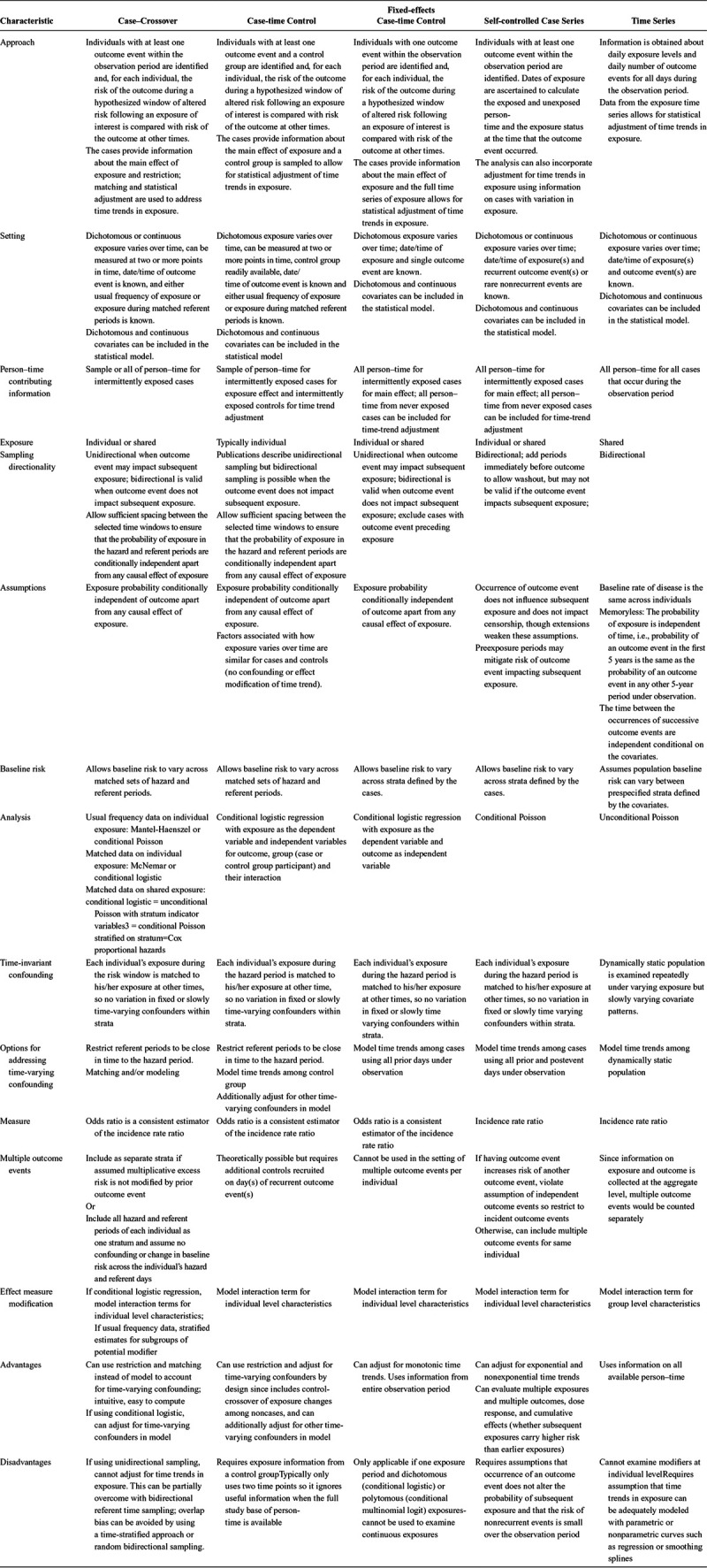
TABLE 2.

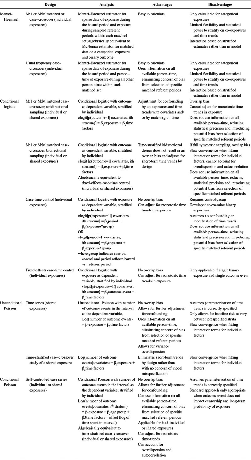
Analytic Approaches for Self-matched Studies

CONDITIONAL EXCHANGEABILITY FOR SELF-MATCHED DATA

In a randomized crossover experiment, each participant receives different interventions at different times during the trial, and the order in which each individual receives the exposures is determined by random allocation. An analysis matched on the individual compares outcomes under different exposure regimes. The investigators design the study to compare exposed and unexposed periods that are close in time so that the probability of the outcome independently of exposure is expected to be the same across the time periods (e.g. the participants’ age and underlying health is not progressing), and they include sufficiently long washout periods to minimize the risk of carryover effect of treatment in the first phase on outcomes in the second phase. In this setting, the exposed and unexposed times under comparison are assumed to be exchangeable; after accounting for any causal effect of exposure on outcome, the probability of the outcome is identical. Therefore, any difference in risk across the time periods is expected to be attributable to the causal effect of the exposure.

When randomization is infeasible or unethical, there are several approaches to examine causal effects of exposures that vary over time within individuals. However, in the observational setting, exposure is determined by the individual or imposed by society or the natural environment rather than by randomization. Therefore, sources of nonexchangeability can threaten the validity of the study. Time-varying confounding can arise due to temporal changes in the risk of the outcome related to the timing of exposure. Selection bias can occur if referent periods for each individual are not sampled independent of their exposure. These sources of nonexchangeability are addressed in the design and analysis of self-matched data.¹⁵ Similar to a randomized crossover experiment, the analysis may be restricted to fairly short time windows so that the baseline risk of the outcome is assumed to be constant across the times under comparison, and washout periods between the time windows may be used to minimize a carryover effect. Just as in cohort and case-control studies, we account for common causes of exposure and outcome (confounding) using restriction, matching and statistical adjustment to achieve conditional exchangeability within levels of the measured confounders.

APPROACHES FOR EXAMINING SELF-MATCHED DATA

Some self-matched approaches compare all exposed person–time to all unexposed person–time for each individual, and some approaches sample some of the eligible person–time (Figure 1). This is directly analogous to the identical objective of a cohort study comparing all exposed and unexposed person–time across individuals and a case-control study comparing an efficient sampling from the underlying study base to answer the same question—whether the outcome rate can be attributed to the exposure.¹⁶ Despite the common goal, each self-matched approach uses different techniques to attain conditional exchangeability between the time periods under comparison.

FIGURE.

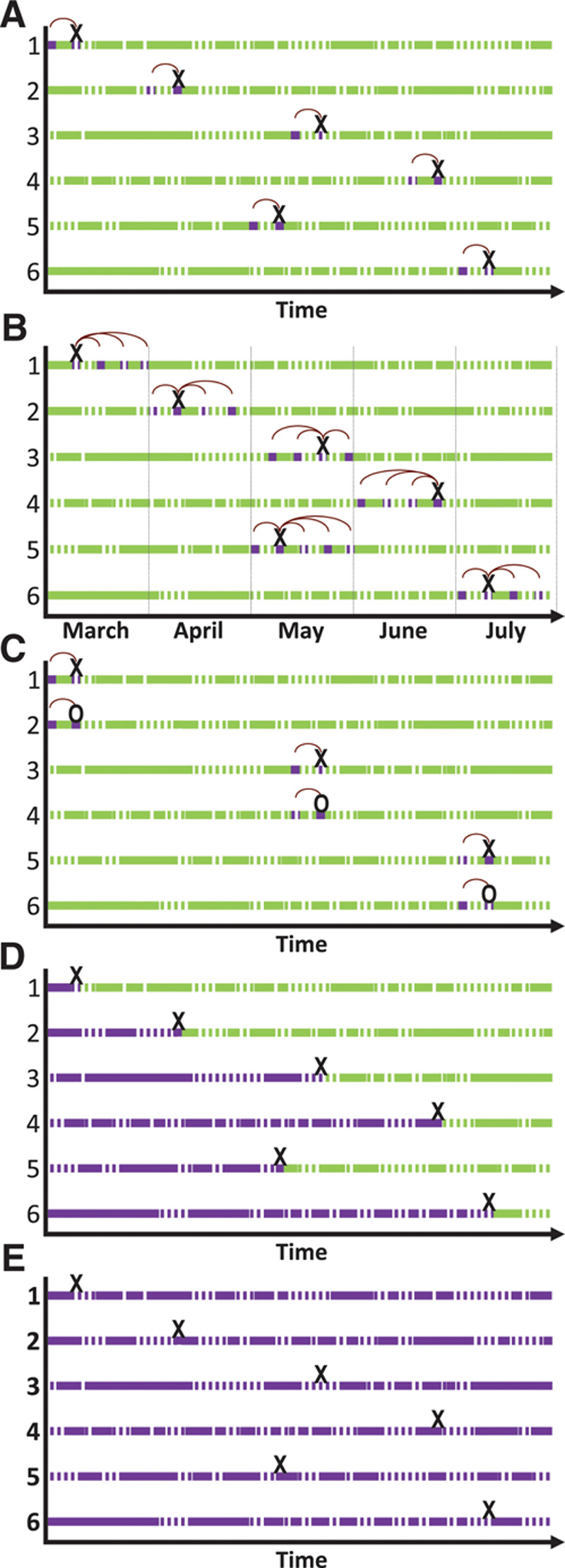
Options for self-matched analyses. Hypothetical data for six individuals. Solid lines represent exposed person–time and dashed lines represent unexposed person–time. Dark shading represents time included in the analysis and light shading represents time excluded from the analysis. An “X” represents the time of the outcome event for each case and an “O” represents the time when someone was sampled as a control. The vertical dashed line represents stratification by time (month). Vertical lines for further stratification could be added to any of these figures because all approaches allow for further adjustment for time-varying factors. Arches represent the referent periods sampled to be close in time to the hazard periods. Each panel represents an example with no censoring, but can be extended to situations with left and/or right censoring. All approaches can be conducted with exposures ascertained prospectively or retrospectively for individual or shared exposures. A, Unidirectional case-crossover with one referent period sampled for each outcome event. Additional referent periods before the outcome event can also be included. In this example, #5 would not contribute information to the estimate because the individual was exposed during the hazard and referent period. B, Time-stratified bidirectional case–crossover. Stratification by time (month) before sampling the referent periods as all days falling on the same day of the week in the same month as the outcome event. Randomly sampling a referent period before or after the hazard period (semisymmetrical bidirectional sampling) or including all recent days other than the hazard period as the referent times (full stratum bidirectional sampling) also avoid overlap bias. C, Case-time control to account for population-level trends in exposure using a sample of controls. The approach was developed for analyses using unidirectional sampling but could theoretically be used with semisymmetric bidirectional sampling. D, Fixed-effects case-time control and self-controlled case-series data for all person–time before the outcome event. A case–crossover analysis of usual frequency data includes this person–time, but exposure is summarized as typical frequency rather than using each time unit in the analysis. E, Self-controlled case-series and fixed-effects case-time control include all person–time under observation, both before and after the outcome event.

Case-crossover

Maclure⁵ proposed that, similar to a randomized crossover experiment, treatment effects can be estimated in an observational setting by comparing each participant’s exposure immediately before the outcome event (referred to as the case period or hazard period) with that individual’s exposure at other times (referred to as the control periods or referent periods). The referent periods must be close enough to the hazard period to ensure that the assumption of exchangeability is met, but far enough in time from the hazard period to prevent short-term autocorrelation and carryover effects within an individual.

In the initial studies using this approach, patients were recruited after events occurred, and they retrospectively reported their usual frequency of past exposure as an estimate of exposure during the entire observation period.^17,18 For instance, patients admitted for a myocardial infarction (MI) were asked about marijuana use immediately before the MI (the hazard period) and about their typical frequency of marijuana use in the past year (the referent period). Because the referent period is restricted to times close to the hazard period, the baseline risk of the outcome is expected to be similar, but within-person confounding due to short-term changes in exposure and outcome risk is not easily addressed. The data are analyzed using a Mantel-Haenszel measure that is efficient for sparse data, which is necessary here because each stratum includes data from only one individual. It only requires the assumption that, conditional on the causal effect of exposure on outcome, the probability of outcome is the same for the hazard period and each of the matched referent periods (pairwise exchangeability).¹⁹ However, this approach is only useful for categorical exposures, it relies on a summary of prior exposure rather than more finely resolved data, and the statistical power to jointly stratify on the individual and on time-varying factors may be limited by the practicality of data collection.

To reduce confounding by time-varying factors such as circadian rhythm, day of week, or co-exposure to other factors that may impact outcome risk, matched interval sampling is used to compare the risk of the outcome, conditional on exposure, during the hazard period to the risk in one or more referent periods matched on some time factor for each individual.²⁰ For example, in a study examining whether coffee intake triggers an MI, there is a higher risk of cardiovascular events in the morning and people are more likely to drink coffee in the morning than at other times of day. Therefore, the heightened risk may be at least partially due to the time of day rather than to the coffee intake. To address this concern, exposure in the hour before MI is compared with exposure in matched referent periods at the same time of day on prior days, or time is included as a covariate in the model.²⁰ Other time-varying factors can be also be addressed by statistical adjustment. For instance, covariates for co-exposure to physical activity can be included in the regression model.

Analyses of matched referent periods are commonly conducted using routinely collected data with high temporal resolution to account for time-varying factors. When experiencing an outcome event impacts subsequent exposure, reverse causation may occur so only times preceding the outcome event are selected as referent periods (unidirectional sampling); otherwise, times before and after the hazard period can be used (bidirectional sampling). Matched interval data are analyzed with conditional logistic regression, allowing for continuous exposures and confounders. Compared with an analysis of usual frequency data with a Mantel-Haenszel estimator, this often yields greater flexibility to adjust for covariates, but only a sample of referent person–time is included so it typically has less statistical efficiency.²⁰ Furthermore, stronger assumptions are necessary when there are two or more referent periods per case. In addition to pairwise exchangeability between the hazard period and each referent period, the probability of outcome must be independent across all periods within a matched set conditional on the causal effect of exposure on outcome (global exchangeability).¹⁹ Second, there can be no dependence (autocorrelation) in exposure over time. A third concern is the issue of overlap bias.²¹ The conditional likelihood formula for conditional logistic regression reflects the probability of the observed data configuration relative to the probability of all possible permutations of the data. If referent periods always precede the outcome event or if referents are systematically selected at specific intervals before and after the outcome event, overlap bias arises because the referent periods are a function of the outcome event times.^21,22

Case-time Control

The case-time control approach was developed for pharmacoepidemiologic research, where confounding by indication is a great challenge. Therefore, a self-matched approach is appealing. Typically, unidirectional sampling is necessary because experiencing an outcome event likely changes subsequent treatment. In addition to temporal changes in individual-level factors, there are also population-level changes. For instance, the probability of treatment may increase over time as its benefits or risks become widely recognized. If there are time trends in exposure, even in the absence of changes in outcome risk, and hence, no time-varying confounding, there is a problem of selection bias, because rather than selecting referent times that represent the exposure distribution in the underlying study base, referent periods were selected when exposure was systematically different.²³

To address time trends in exposure, Suissa^6,7 proposed the case-time control approach as an extension of the case-crossover technique. Cases and a sample of noncases (controls) at risk at the time the case occurred are recruited at the time of the cases’ outcome event as in a risk-set sampling paradigm, and information on a dichotomous exposure during the hazard period and an earlier referent period is obtained for all participants. The data are analyzed using conditional logistic regression. However, rather than the conventional approach of estimating the odds of the outcome, exposure is modeled as the dependent variable and outcome and time factors are included as predictors, with the model stratified by individual. In an intuitive mathematically identical parameterization, the model includes period (hazard or referent) as the dependent variable with independent variables for exposure and an interaction term for exposure and group (case or control). The association for the controls is estimated by the coefficient for exposure as a function of time period, which if there were no time trend in exposure would be null. The interaction term corresponds to the self-matched exposure effect based on the cases adjusted for the self-matched time (period) effect estimated among the controls.

The design has been criticized because it assumes the same time trend in exposure for cases and controls.^7,23 This is analogous to difference-in differences estimators in econometrics²⁴ that require the assumption that, in the absence of treatment, the average outcomes for the treated and untreated groups would have followed parallel trends over time. These assumptions are unverifiable in a standard case-time control study, because it is restricted to intermittently exposed cases and controls at two time points. However, one could examine whether the time trends are different between cases and controls if the sample were nested within a population-based registry or other well-defined cohort. Another drawback is that it was developed for data with one hazard period and one referent period. If all person–time during the observation period is available, accounting for time trends using only a sample of controls and only two time points may not maximally use the richness of the data. Despite these limitations, if data on an appropriate control group is available, it provides a valid and easy computational method for conducting a self-matched analysis with unidirectional sampling that accounts for time trends in exposure and is free from overlap bias.

A subsequent variant of the case-time control design²⁵ aimed to address time trends in exposure using data restricted to cases and referent times preceding the outcome event. However, if exposure impacts survival, this approach is likely to induce selection bias by modeling time trends based on the exposure distribution among future cases rather than a sample that represents exposure in the underlying study base. Furthermore, when exposure and outcome are associated, referent times selected from future cases are more likely to be unexposed times, inducing a bias from sampling referent times dependent on exposure. This limits the utility of this approach, and may be particularly problematic in the setting of pharmacoepidemiology.

Fixed-effects Case-time Control

To address the limitations of the case-time control approach, Allison and Christiakis⁸ proposed a method that also models exposure status as the dependent variable in a conditional logistic regression model to adjust for time trends in exposure, but it only requires information on cases and utilizes all person–time under observation before the outcome event. For each case, there is one row of data for each day of observation. If observation continues after the outcome event, the data are analyzed with a conventional conditional logistic regression model. If occurrence of the outcome event is a censoring event (e.g. death), a standard conditional logistic model would not converge because the outcome event is always the last observation for each participant. Therefore, the case-time-control technique of reversing the dependent and independent variables in the conditional logistic regression model is applied. This approach is only applicable for a dichotomous exposure, though a multinomial logit model for polytomous exposures should be possible. When appropriate, it offers several advantages. Unlike a unidirectional case–crossover analysis, there is no concern of overlap bias because the dependent variable is not perfectly predicted by time, and adjustment for monotonic functions of time is possible. Unlike the case-time control approach, there is no need to obtain information on controls.

Self-controlled Case Series

Farrington⁹ proposed the self-controlled case series approach that uses all person–time both before and after the outcome event. A dataset is created with person–time for each case partitioned into exposed and unexposed intervals. To attain exchangeability, the data are further divided by time-varying factors that are strong predictors of exposure and outcome, such as age. In the standard approach, the data are analyzed with a conditional Poisson model stratifying on the individual with the number of outcome events as the response variable and the log of each interval length as an offset. This is mathematically identical to a multinomial or fixed effect model.²⁶ This approach uses all of the person–time under observation, it does not require the assumption of global exchangeability, and overlap bias does not occur. Semiparametric extensions using conditional Poisson²⁷ or Cox stratified proportional hazards models²⁸ were designed to avoid misspecification of the baseline incidence.

In this approach, it is assumed that within individuals, outcome events are recurrent and independent of each other or rare and nonrecurrent, and that occurrence of an outcome event does not alter the probability of subsequent exposure. If experiencing an event temporarily alters exposure, adjustment for the immediate preexposure period removes this person–time from the referent information. If each individual experiences one episode of exposure, this problem could be addressed by redefining the beginning of observation as the start of exposure time, with some loss in statistical power.¹⁰ Alternatively, for dichotomous exposures with short postexposure risk, a pseudo-likelihood approach can be used to reclassify postevent exposure time. The final assumption is that the occurrence of an outcome event does not impact the censoring of the observation period. Extensions have been developed to address violations of changes in postevent exposure²⁹ or censoring.^30,31

SELECTING THE OPTIMAL SELF-MATCHED APPROACH AND ANALYSIS

All self-matched techniques examine the acute risk of an outcome event following transient exposure to a potential trigger by comparing risk among each individual at different times, assuming no misclassification of exposure, outcome, or covariates. Similar to matched cohort and case-control studies, all of these approaches are susceptible to greater bias from nondifferential exposure misclassification than analyses that do not require matching.^32,33 In all approaches, as with any study design, the etiologically relevant hazard period may be immediately before the outcome event or may involve time lags. All regression models for self-matched data provide an estimate of the relative risk assuming a constant baseline incidence within categories of the specified time-varying factors for each individual.^10,19 They all adjust implicitly for exponential time trends in the baseline incidence and account for other nonmonotone time-trends with parametric terms.¹⁹ The case-time control and fixed-effects case-time control can also include covariates for monotonic time trends. There are, however, several factors to consider when selecting an approach for analyzing self-matched data.

Changes in Exposure and Outcome

The concern of time-varying confounding depends on the substantive question of interest and on the composition of the study base. There may be little concern of confounding in a study conducted on an open cohort of individuals hospitalized at a local hospital over a relatively short follow-up period. However, an aging closed cohort may involve concerns that there are factors that systematically change in a manner related to exposure and outcome. For instance, in a self-matched study examining the acute risk of MI following the death of a spouse, individuals in a closed cohort are aging over time, with a potentially corresponding higher probability of experiencing the death of a spouse and a higher probability of experiencing an MI.

Person–time Contributing Information

The exposure effect in all self-matched approaches is based on cases, but the individuals who contribute information differ. A case–crossover analysis with usual frequency data is restricted to intermittently exposed cases, and a case–crossover study with matched interval data is restricted to cases with exposures that are discordant for the hazard period and at least one of the matched referent periods. The case-time control approach includes individuals who were not cases at the time of inclusion in the study (controls), and the fixed-effects case-time control and self-controlled case series approaches include cases whose exposure remains constant during the observation period to model changes in the risk of the outcome over time. If it is necessary to account for the effect of long-lasting or monotone exposures, unexposed cases may be required to separate age and exposure effects.²⁷ Including cases with constant exposure could theoretically be included to estimate time trends in a case–crossover analysis. The differences in who contributes information may impact the internal validity and generalizability of the results because cases that are never exposed during long observation periods may be different from people with variation in exposure during the study. In these situations, restricting the sample to people who were exposed at some time over the observation period may result in lower precision and limit generalizability, but it may improve internal validity⁸ and avoid violations of the positivity requirement that there are exposed and unexposed participants for each value of the covariates.³⁴

Exposure, Confounder, and Outcome Assessment

In all self-matched approaches, exposure may be recorded prospectively before outcomes occur, such as data obtained with self-report daily questionnaires, electronic health records, administrative records, or meteorologic surveillance with local monitors. Alternatively, exposure data may be ascertained retrospectively after the onset of the outcome. For instance, information may be obtained via. interviews upon hospitalization for the outcome event or medical record review after identifying arrhythmias from implantable defibrillators.

The study may involve self-reported exposures and outcomes, such as anger outbursts, alcohol intake, or physical activity, or they can be conducted using objectively recorded data from sources such as sleep polysomnography³⁵ and actigraphy monitors. Routinely collected data are immensely useful; phone billing records³⁶ include data on the timing of cell phone use; administrative health datasets often include information on dates of prescription drug orders and dispensed doses, vaccinations, and procedures; and national registries often have information on inpatient and outpatient diagnoses. If data have already been collected for a well-defined cohort over many years, the choice among self-matched approaches may depend on how the investigator prefers to minimize bias due to time-varying factors. These methods include matching restriction to periods close in time and statistical adjustment (case–crossover), a control group and further matching; restriction and statistical adjustment (case–time control); statistical adjustment in a conditional Poisson (self-controlled case–series); or discrete-time modeling (fixed-effects case–time control).

Total Observation Period versus a Sample of the Observation Period

Some case–crossover and case–time control studies use a sample of person–time that may seem analogous to case-control studies, whereas the fixed-effects case–time control and self-controlled case-series approaches use all of the person–time in the observation period, which may seem analogous to cohort studies. However, as we have discussed previously,¹⁵ a study using all of the person–time under observation may garner greater statistical precision than a study using a sample of the person–time,³⁷ but in the absence of confounding and selection bias, both approaches yield identical results in expectation because all case-control studies can be conceptualized as an efficient sampling from the underlying, possibly hypothetical, pool of person–time.^16,38

Given this equivalence, the choice between using a sample or all of the person–time depends on the ability to address time-varying factors. One option is to select referent periods that are close in time to the hazard period to minimize concerns of time-varying confounding by changes in baseline risk but spaced far enough apart to prevent carryover effects and autocorrelation.¹⁵ Selecting more referent periods per case may yield greater statistical precision, but may result in greater risk of autocorrelation between referent periods. Furthermore, selecting one referent period for each hazard period only requires the assumption of pairwise exchangeability, but selecting two or more referent periods requires the stronger assumption of global exchangeability.¹⁹

An analysis using all person–time can improve statistical efficiency and prevent selection bias arising from incorrectly sampling referent times when individuals are more or less likely to be exposed. To minimize time-varying confounding, the investigator parameterizes time-trends in multivariable models with indicator variables, polynomials, or splines for time-varying factors such as season, age, or policy changes. This allows for flexibility in handling time trends beyond what is possible with matching on discrete time blocks, but there may be a greater concern of long-term trends in exposures and confounders for studies where individuals contribute person–time for many years, and one must assume that the shape of the time trends are correctly specified.

Impact of Outcome Events on Subsequent Exposure

Experiencing an outcome event may affect subsequent exposure. For instance, having an MI may lead to less physical activity and changes in medication use. In this situation, including postevent referent times leads to reverse causation. For example, if outcome decreases subsequent exposure, it would lead to an upward bias if postevent times were included. In a self-controlled case-series analysis, postevent changes in exposure are addressed by including a term for the immediate preexposure period, by redefining the beginning of the observation period as the start of a single exposure time under observation, or by using a technique that reclassifies postevent exposure time as unexposed time with the number of events estimated from other unexposed times. In a case-crossover, case-time control or fixed-effects case-time control analysis, this is addressed by selecting all referent periods from times preceding the hazard period (unidirectional sampling).

If unidirectional sampling is appropriate, a case-crossover analysis can be conducted with either a Mantel-Haenszel measure for usual frequency data or conditional logistic regression for matched interval data, though the latter may lead to overlap bias.²² In a unidirectional case–crossover analysis, changes in the probability of exposure between the hazard and referent period(s) may induce selection bias because the selected referent times have a systematically different exposure distribution than the underlying study base.²³ Conditional logistic regression can be used with the case-time control and fixed-effects case-time control approaches to address selection bias from time trends in exposure. In these analyses, the dependent variable is exposure, so the fact that the referent periods systematically precede the outcome no longer induces overlap bias.

Bidirectional sampling is appropriate when experiencing the outcome event does not impact subsequent long-term exposure. For instance, in a study of coffee intake and the occurrence of migraines, a regular coffee drinker may resume their daily habit regardless of whether they recently suffered a migraine. Similarly, having an MI does not impact subsequent population levels of ambient pollution or weather. Therefore, in these situations, bidirectional sampling can be used to include either a sample or all available person–time before and after the outcome occurs.

Several approaches use a sample of person–time, either randomly sampling a referent period before or after the hazard period (semisymmetrical bidirectional sampling),³⁹ including all recent days other than the hazard period as the referent times (full stratum bidirectional sampling),⁴⁰ or most commonly, selecting referent times on the same day of the week within the same calendar month as the hazard period (bidirectional time-stratified sampling).⁴¹ Bidirectional sampling may improve statistical efficiency by including more referent periods per hazard period, it overcomes the problems of overlap bias and confounding by slowly varying characteristics^39,41 in a time-stratified or full stratum case–crossover analysis, and it is a requirement for standard self-controlled case-series analyses.

Individual and Shared Exposures

Self-matched analyses can be conducted for individual exposures such as medication use and lifestyle factors, and it can be used to study exposures shared across individuals such as ambient pollution. In studies of individual exposures and fatal outcomes, unidirectional sampling is typically used. In studies of shared exposures, bidirectional sampling is appropriate even though the individual is no longer at risk of a subsequent event, because referent periods selected after the outcome event still represent the exposure distribution in the underlying study base.^15,42

In analyses of shared exposures, potential confounders are factors that change over time in a manner related to fluctuations in the exposure and outcome at a population level, such as environmental factors. Therefore, functions of time are included in the regression model with indicator variables, periodic (sine/cosine) functions, or flexible splines. In studies of individual exposures, there is no concern of a correlation in exposure or outcome between individuals, but in studies of shared exposures, the assumption that there is no correlation in the number of events (i.e., between strata) must also be considered. If events are not independent and there is clustering by day, this autocorrelation in events may lead to overdispersion.

There are several techniques for studying shared exposures. Typically, the dataset for a time-stratified bidirectional case–crossover analysis includes rows for each hazard and each referent period per case. This expanded layout can result in large datasets when there are many cases, and it has slow convergence when fitting interaction terms for individual-level modifiers. Because several cases occur each day with the same shared exposure level, a more compact semiexpanded dataset includes a row for each day and a row for each of its matched referent days, with a count of events on those days. For both layouts, the data are analyzed with a conditional logistic regression model stratified by the event date, and the semiexpanded data are weighted by event frequency. The approach is intuitive for comparing hazard and referent days, and it allows for examination of individual-level modifiers, but there is no ability to account for overdispersion or autocorrelation in the outcome.

An alternative computationally efficient approach can be conducted using a compact data set with one row for each day with at least one event and measures of exposure, time-varying factors, and the number of events on that day. By assuming that the population size remains fairly stable over the time scale under analysis, the denominator of total population size is not needed. Although it is not self-matched, this aggregated time series data accomplish the same goal as the self-matched approaches; it eliminates confounding by fixed or slowly varying factors, such as population age distribution or socioeconomic position. If analyzed with unconditional Poisson regression, only group-level modifiers can be examined. If analyzed with a conditional Poisson model, individual-level modifiers can be included, but either way, all of the person–time under observation is included and the model can account for overdispersion or autocorrelation.^3,43

The results of a full-stratum bidirectional or time-stratified case–crossover study using conditional logistic regression are mathematically equivalent to the results of a time series study using unconditional Poisson regression with indicator variables for strata of time,^3,22,44 where the smooth function of time is assumed to be a step function with a separate level of baseline risk for each prespecified stratum.²² It is also equivalent to a conditional Poisson model conditioned on the number of outcome events in each stratum, and the latter allows for overdispersion, autocorrelation, and varying rate denominators.⁴³

Compared with a time-series analysis using unconditional Poisson regression, a case–crossover analysis using conditional logistic regression offers an intuitive conceptualization of the comparison of interest, providing insight that could be missed when analyzing aggregated daily data with complex multivariable models that include nonlinear terms for time trends.⁴⁵ Also, it is more suitable for examining potential modifiers of the association to identify characteristics of individuals who are particularly susceptible to adverse health effects or are more likely to benefit from healthful exposures. Conversely, a time-series approach is often more computationally straightforward because aggregated data are typically readily available from existing data sources, and the analysis allows for overdispersion and autocorrelation.

CONCLUSION

In all self-matched approaches, exposure and outcome information may be collected prospectively or retrospectively, and they may be ascertained objectively or via. self-report. The validity of all self-matched analyses relies on the assumption that, conditional on the causal effect of exposure on outcome, there are no temporal changes in the risk of the outcome related to the timing of exposure. Different techniques aim to attain this comparability in different ways: matching, restriction to periods close in time, and statistical adjustment (case–crossover), a control group and further matching, restriction and statistical adjustment (case-time control) or statistical adjustment in a conditional Poisson (self-controlled case-series) or discrete-time model (fixed-effects case-time control).

Prior Presentation

Some of these ideas were presented in a presentation for the Society for Epidemiologic Research Epidemiologic Methodology Applications Conference on November 17, 2012.

REFERENCES

- 1.Armstrong BG. Fixed factors that modify the effects of time-varying factors: applying the case-only approach. Epidemiology. 2003;14:467–472.. [DOI] [PubMed] [Google Scholar]
- 2.Smeeth L, Donnan PT, Cook DG. The use of primary care databases: case-control and case-only designs. Fam Pract. 2006;23:597–604.. [DOI] [PubMed] [Google Scholar]
- 3.Lu Y, Zeger SL. On the equivalence of case-crossover and time series methods in environmental epidemiology. Biostatistics. 2007;8:337–344.. [DOI] [PubMed] [Google Scholar]
- 4.Gault N, Castañeda-Sanabria J, De Rycke Y, et al. Self-controlled designs in pharmacoepidemiology involving electronic healthcare databases: a systematic review. BMC Med Res Methodol. 2017;17:25. [DOI] [PMC free article] [PubMed] [Google Scholar]
- 5.Maclure M. The case-crossover design: a method for studying transient effects on the risk of acute events. Am J Epidemiol. 1991;133:144–153.. [DOI] [PubMed] [Google Scholar]
- 6.Suissa S. The case-time-control design. Epidemiology. 1995;6:248–253.. [DOI] [PubMed] [Google Scholar]
- 7.Suissa S. The case-time-control design: further assumptions and conditions. Epidemiology. 1998;9:441–445.. [PubMed] [Google Scholar]
- 8.Allison PD, Christakis NA. Fixed-effects methods for the analysis of nonrepeated events. Sociol Methodol. 2006;36:155–172.. [Google Scholar]
- 9.Farrington CP. Relative incidence estimation from case series for vaccine safety evaluation. Biometrics. 1995;51:228–235.. [PubMed] [Google Scholar]
- 10.Whitaker HJ, Farrington CP, Spiessens B, et al. Tutorial in biostatistics: the self-controlled case series method. Stat Med. 2006;25:1768–1797.. [DOI] [PubMed] [Google Scholar]
- 11.Aalen OO, Borgan Ø, Keiding N, et al. Interaction between life history events. Nonparametric analysis for prospective and retrospective data in the presence of censoring. Scandinavian J Stat. 1980;7:161–171.. [Google Scholar]
- 12.Prentice RL, Vollmer WM, Kalbfleisch JD. On the use of case series to identify disease risk factors. Biometrics. 1984;40:445–458.. [PubMed] [Google Scholar]
- 13.Feldmann U. Epidemiologic assessment of risks of adverse reactions associated with intermittent exposure. Biometrics. 1993;49:419–428.. [PubMed] [Google Scholar]
- 14.Feldmann U. Design and analysis of drug safety studies, with special reference to sporadic drug use and acute adverse reactions. J Clin Epidemiol. 1993;46:237–244.. [DOI] [PubMed] [Google Scholar]
- 15.Mittleman MA, Mostofsky E. Exchangeability in the case-crossover design. Int J Epidemiol. 2014;43:1645–1655.. [DOI] [PMC free article] [PubMed] [Google Scholar]
- 16.Miettinen O. Estimability and estimation in case-referent studies. Am J Epidemiol. 1976;103:226–235.. [DOI] [PubMed] [Google Scholar]
- 17.Mittleman MA, Maclure M, Tofler GH, et al. Triggering of acute myocardial infarction by heavy physical exertion. Protection against triggering by regular exertion. Determinants of Myocardial Infarction Onset Study Investigators. N Engl J Med. 1993;329:1677–1683.. [DOI] [PubMed] [Google Scholar]
- 18.Mittleman MA, Lewis RA, Maclure M, et al. Triggering myocardial infarction by marijuana. Circulation. 2001;103:2805–2809.. [DOI] [PubMed] [Google Scholar]
- 19.Vines SK, Farrington CP. Within-subject exposure dependency in case-crossover studies. Stat Med. 2001;20:3039–3049.. [DOI] [PubMed] [Google Scholar]
- 20.Mittleman MA, Maclure M, Robins JM. Control sampling strategies for case-crossover studies: an assessment of relative efficiency. Am J Epidemiol. 1995;142:91–98.. [DOI] [PubMed] [Google Scholar]
- 21.Austin H, Flanders WD, Rothman KJ. Bias arising in case-control studies from selection of controls from overlapping groups. Int J Epidemiol. 1989;18:713–716.. [DOI] [PubMed] [Google Scholar]
- 22.Levy D, Lumley T, Sheppard L, et al. Referent selection in case-crossover analyses of acute health effects of air pollution. Epidemiology. 2001;12:186–192.. [DOI] [PubMed] [Google Scholar]
- 23.Greenland S. Confounding and exposure trends in case-crossover and case-time-control designs. Epidemiology. 1996;7:231–239.. [DOI] [PubMed] [Google Scholar]
- 24.Ashenfelter O. Estimating the effect of training programs on earnings. Rev Econ Stat. 1978;60:47–57.. [Google Scholar]
- 25.Wang S, Linkletter C, Maclure M, et al. Future cases as present controls to adjust for exposure trend bias in case-only studies. Epidemiology. 2011;22:568–574.. [DOI] [PMC free article] [PubMed] [Google Scholar]
- 26.Xu S, Zeng C, Newcomer S, et al. Use of fixed effects models to analyze self-controlled case series data in vaccine safety studies. J Biom Biostat. 2012;0:1–5.. [DOI] [PMC free article] [PubMed] [Google Scholar]
- 27.Farrington CP, Whitaker HJ. Semiparametric analysis of case series data. J R Stat Soc Ser C Appl Stat. 2006;55:553–594.. [Google Scholar]
- 28.Xu S, Gargiullo P, Mullooly J, et al. Fitting parametric and semi-parametric conditional Poisson regression models with Cox’s partial likelihood in self-controlled case series and matched cohort studies. J Data Sci. 2010;8:349–360.. [Google Scholar]
- 29.Hua W, Sun G, Dodd CN, et al. A simulation study to compare three self-controlled case series approaches: correction for violation of assumption and evaluation of bias. Pharmacoepidemiol Drug Saf. 2013;22:819–825.. [DOI] [PubMed] [Google Scholar]
- 30.Farrington CP, Whitaker HJ, Hocine MN. Case series analysis for censored, perturbed, or curtailed post-event exposures. Biostatistics. 2009;10:3–16.. [DOI] [PubMed] [Google Scholar]
- 31.Farrington CP, Anaya-Izquierdo K, Whitaker HJ, et al. Self-controlled case series analysis with event-dependent observation periods. J Am Stat Assoc. 2011;106:417–426.. [Google Scholar]
- 32.Greenland S. The effect of misclassification in matched-pair case-control studies. Am J Epidemiol. 1982;116:402–406.. [DOI] [PubMed] [Google Scholar]
- 33.Frisell T, Öberg S, Kuja-Halkola R, et al. Sibling comparison designs: bias from non-shared confounders and measurement error. Epidemiology. 2012;23:713–720.. [DOI] [PubMed] [Google Scholar]
- 34.Hernán MA, Robins JM. Estimating causal effects from epidemiological data. J Epidemiol Community Health. 2006;60:578–586.. [DOI] [PMC free article] [PubMed] [Google Scholar]
- 35.Monahan K, Storfer-Isser A, Mehra R, et al. Triggering of nocturnal arrhythmias by sleep-disordered breathing events. J Am Coll Cardiol. 2009;54:1797–1804.. [DOI] [PMC free article] [PubMed] [Google Scholar]
- 36.Redelmeier DA, Tibshirani RJ. Association between cellular-telephone calls and motor vehicle collisions. N Engl J Med. 1997;336:453–458.. [DOI] [PubMed] [Google Scholar]
- 37.Breslow NE, Day NE. Statistical methods in cancer research. Volume I - The analysis of case-control studies. IARC Sci Publ. 1980:5–338.. [PubMed] [Google Scholar]
- 38.Wacholder S, McLaughlin JK, Silverman DT, et al. Selection of controls in case-control studies. I. Principles. Am J Epidemiol. 1992;135:1019–1028.. [DOI] [PubMed] [Google Scholar]
- 39.Navidi W, Weinhandl E. Risk set sampling for case-crossover designs. Epidemiology. 2002;13:100–105.. [DOI] [PubMed] [Google Scholar]
- 40.Navidi W. Bidirectional case-crossover designs for exposures with time trends. Biometrics. 1998;54:596–605.. [PubMed] [Google Scholar]
- 41.Lumley T, Levy D. Bias in the case-crossover design: implications for studies of air pollution. Environmetrics. 2000;11:689–704.. [Google Scholar]
- 42.Miettinen OS, Cook EF. Confounding: essence and detection. Am J Epidemiol. 1981;114:593–603.. [DOI] [PubMed] [Google Scholar]
- 43.Armstrong BG, Gasparrini A, Tobias A. Conditional Poisson models: a flexible alternative to conditional logistic case cross-over analysis. BMC Med Res Methodol. 2014;14:122. [DOI] [PMC free article] [PubMed] [Google Scholar]
- 44.Navidi W. Poisson regression and the case-crossover design: similarities and differences. Commun Stat Theory Methods. 2008;37:213–220.. [Google Scholar]
- 45.Maclure M, Mittleman MA. Case-crossover designs compared with dynamic follow-up designs. Epidemiology. 2008;19:176–178.. [DOI] [PubMed] [Google Scholar]