RNA-seq: Basic Bioinformatics Analysis

Abstract

Quantitative analysis of gene expression is crucial for understanding the molecular mechanisms underlying genome regulation. RNA-seq is a powerful platform for comprehensive investigation of the transcriptome. In this Unit, we present a general bioinformatics workflow for the quantitative analysis of RNA-seq data and describe a few current publicly available computational tools applicable at various steps of this workflow. These tools comprise a pipeline for quality assessment and quantitation of RNA-seq data that starts from raw sequencing files and is focused on the identification and analysis of genes that are differentially expressed between biological conditions.

INTRODUCTION

Quantifying gene expression and identifying transcripts that are differentially expressed between two conditions in a cell, tissue, or organism is an important approach to deciphering the molecular physiology of the cell. RNA-seq analysis based on next-generation sequencing (NGS) data has recently become the de facto standard for the analysis of gene expression at the level of the whole transcriptome. This analysis is often crucial for the generation of mechanistic hypotheses about molecular events in cells and tissues. Examples include cellular responses to physiological stimuli, effects of experimental perturbations on specific genes and pathways, or the malfunction of gene regulation in disease. RNA-seq involves isolation of total RNA from tissues or cells of interest followed by the construction of DNA libraries and sequencing of these libraries using a next-generation sequencing instrument.

This Unit covers a basic computational workflow of bioinformatics analysis of RNA-seq data. The focus is on basic computational analysis of traditional RNA-seq data, and does not cover single-cell RNA-seq, small RNA-seq, GRO-seq, or other specialized RNA-seq applications. The workflow described below requires installation of and basic familiarity with Unix/Linux and R command-line interfaces.

The workflow includes three parts: (a) mapping sequencing reads to a reference genome or transcriptome; (b) quantifying expression levels of individual genes and transcripts; and (c) identifying specific genes and transcripts that are differentially expressed between samples. The resulting sets of differentially expressed genes can be further analyzed, either manually or automatically, for example, for the presence of relevant genes of interest, enrichment of functional gene categories, or overlap with sets of genes or regulatory genomic elements identified in other experiments.

STRATEGIC PLANNING

Meaningful experimental design is essential for successful RNA-seq analysis. A key recommendation is to include at least three biological replicates per condition/group, which is crucial for robust estimates of statistical significance in the analysis of differential gene expression. In addition, the samples should be sequenced to sufficient depth. For a basic RNA-seq experiment in a mammalian model with sequencing performed on an Illumina HiSeq, NovaSeq, NextSeq or MiSeq instrument, the recommended number of reads is at least 10 million per sample, and optimally, 20–30 million reads per sample. Lower sequencing depths yield statistically insufficient numbers of reads per transcript and effectively limit statistical analyses to highly expressed genes. Another key issue concerns whether the goal is to quantify expression levels at loci, or to go to greater depth and compare splicing patterns on genes. Paired-end (PE) Illumina sequencing is better suited for capturing splicing events than single-end (SE) sequencing, but is more costly. Finally, 50 bp Illumina reads are typically sufficient for the unique mapping of a mammalian RNA to the genome, but longer reads increase the likelihood of directly capturing splice sites within the reads, thereby improving the analysis of potential alternative splice forms.

BASIC PROTOCOL

Raw RNA-seq data are typically formatted as FASTQ files. FASTQ is a text-based format storing the sequences of the reads as well as their sequencing quality. The file is organized in groups of four lines per read as shown below:

@NB500929:247:HL2TYBGX3:1:11101:25163:1060
GATTTGGGGTTCAAAGCAGTATCGATCAAATAGTAAATCCATTTGTTCAACTCACAGTTT
+
!’’*((((***+))%%%++)(%%%%).1***-+*’’))**55CCF>>>>>>CCCCCCC65

The first line starts with “@” and is followed by a unique sequence identifier, which includes instrument ID (NB500929), run number (247), and flow cell ID (HL2TYBGX3), followed by the numbers specifying the location of the DNA fragment on the flowcell. In the case of paired-end sequencing, two FASTQ files for read 1 and read 2 include the same sequence identifiers plus the read number (1 or 2), which indicates whether the sequence comes from read 1 or read 2 of the DNA fragment. The second line contains the read sequence. The third line starts with a “+” character and can optionally be followed by the same sequence identifier and any additional description. The fourth line encodes the sequencing quality scores for each base, which are coded as individual symbols according to a coding scheme (see https://support.illumina.com/help/BaseSpace_OLH_009008/Content/Source/Informatics/BS/QualityScoreEncoding_swBS.htm)

Alignment is the computational process of mapping the sequence of each read to a reference genome using a specific annotation of genes and other genomic elements generated, for example, by the ENSEMBL project (Zerbino et al., 2017). Compared to the alignment performed in whole-genome sequencing and other applications, a challenge of mapping short-read RNA-seq data comes from the non-contiguous structure of eukaryotic transcripts along genomic coordinates. This challenge requires special algorithmic treatment of the cases when the 5’ and 3’ parts of a read sequence correspond to two different exons, or when reads from two ends of the same library fragment are mapped to non-adjacent exons in the reference transcript. In this protocol, we describe the use of the STAR alignment tool (Dobin et al., 2013) as it provides relatively high alignment speed and lower mapping error rates.

After mapping reads to the genome, it is important to survey the quality of the RNA-seq data in more depth. This can be accomplished using standard software tools, for example Picard (http://broadinstitute.github.io/picard), Qualimap2 (Okonechnikov et al. 2016), RNASeQC (DeLuca et al. 2012), or SAMTools (Li et al. 2009). The workflow described in this UNIT uses Picard (http://broadinstitute.github.io/picard). Picard generates various “conglomerate” metrics of the mapped reads in a given sample. These metrics include the fractions of total nucleotide bases in the reads that map to annotated exons, introns, UTRs, and intergenic regions bases aligned to mRNA regions, the rate of read duplication (fraction of redundant reads mapping to the same genomic coordinates) etc. This step is essential for assessing the quality of sequencing libraries and diagnosing potential issues with RNA extraction, library construction, or sequencing. After resolving potential quality issues and removing low-quality samples, the workflow proceeds to the quantitation of reads mapped to individual transcripts and identification of differentially expressed genes.

Necessary Resources

Download and install the required tools:

• STAR: https://github.com/alexdobin/STAR

• Picard: https://broadinstitute.github.io/picard/

• HTseq: https://htseq.readthedocs.io/en/release_0.9.1/install.html

• R: https://www.r-project.org

• HARDWARE:

  Computer with Unix, Linux, or Mac OS X operating systems. RAM requirements are at least 10 × genome size bytes for STAR alignment. A human genome of ~3 gigabases (Gbp) will require ~30 gigabytes (GB) of RAM. 32 GB is recommended for human genome alignments. Consecutive STAR jobs with the same reference genome can be run using shared memory using –genomeLoad LoadAndKeep command option, which saves the time required to load the reference index for each job. It is also necessary to have sufficient storage space (>100Gb) for output files

• 1. Download the reference genome as a DNA FASTA file and the gene annotation GTF file from the Ensembl database: https://useast.ensembl.org/info/data/ftp/index.html

• 2. Open a Unix/Linux command line environment (“Terminal” application in a Linux operating system or macOS). Create the alignment index of the reference genome using the STAR index utility as described at the following website: https://github.com/alexdobin/STAR; using the following command:

  STAR --runMode genomeGenerate --genomeDir <reference directory> --genomeFastaFiles <reference genome fasta file> --sjdbGTFfile <reference genome gtf file> --sjdbOverhang 49

  For example, for genome reference fasta file “Homo_sapiens.GRCh38.dna.fa” and gene annotation file “Homo_sapiens.GRCh38.92.gtf” downloaded in step 1, use the following command to create the reference STAR index:

  STAR --runMode genomeGenerate --genomeDir human_GRCh38 --genomeFastaFiles Homo_sapiens.GRCh38.dna.fa --sjdbGTFfile Homo_sapiens.GRCh38.92.gtf --sjdbOverhang 49

  A more detailed protocol for STAR usage is described in Dobin and Gingeras, 2015.

• 3. Download the set of custom wrapper scripts from https://github.com/MolBioBioinformatics/RNA_seq_analysis. This set includes three Perl scripts (RNAseq_align.pl, RNAseq_qc.pl, and RNAseq_count.pl) and two examples of input files with local configuration of required computational tools (configure.txt) and the list of input samples (sample_list.txt).

• 4. Edit the tab-delimited configuration file (configure.txt), which was downloaded at step 3.

  This file contains a tab-delimited table (Table 1) that indicates the names and locations on the user’s machine (full local file paths) of the three required tools, STAR, Picard, and HTseq installed before starting the protocol; the GTF file with genome annotation downloaded at step 1; the directory with the STAR reference files generated at step 2; and the directory with the input FASTQ files. To determine the full path to a standard pre-installed package in a Unix/Linux environment, one can use the “which” command, for example:

  $ which STAR
  /usr/local/bin/STAR

• 5. Edit the tab-delimited input list in file sample.list, which was downloaded at step 3.

  This file contains a tab-delimited table (Table 2) that indicates the group assignment, the name of the sample, and the name of the corresponding FASTQ file for each experimental sample. In the example shown in Table 2, there is a total of 6 RNA samples that form two groups of biological triplicates: samples from wild-type (marked WT) and mutant cells (marked mut). The gene expression in the “WT” group will be compared to the gene expression in the “mut” group, and differentially expressed genes will be identified at the later steps of the workflow. Specific group names (the first column) and sample names (the second column) can be arbitrary, whereas file names (the third column) should be the exact names of the input FASTQ files that are located in the directory whose full path is listed as FASTQ_DIR in the configuration file (Table 1). In the case of paired-end sequencing when two FASTQ files are produced for each sample, this table should be extended into four columns, with the fourth column indicating the name of the second FASTQ file for each sample.

• 6. From the directory that contains the downloaded scripts (step 3) and edited files confirgure.txt (step 4) and sample_list.txt (step 5), use the following command to run the alignment:

  ./RNAseq_align.pl sample_list.txt configure.txt

  This step will map the reads from the input FASTQ files to the reference genome using the STAR aligner. Once it is completed, this step will generate several subdirectories that correspond to each individual sample and are named by sample names listed in the file sample_list.txt (Table 2), for example “WT.RNA.rep1”. Each subdirectory will contain the generated STAR alignments as BAM formatted files. The completion of this command may take several hours. This time will depend on the number of samples, the number of reads, genome size, and the CPU capacity of the particular machine.

Table 1.

Example of the configuration table (file configure.txt)

STAR	/usr/local/bin/STAR
Picard	/home/ji/tools/picard-tools/picard-tools-1.100
HTseq	/home/ji/.local/bin/htseq-count
GTF	/home/ji/data/CPMB/pipeline_RNA/ref/gtf
STAR_REF	/home/ji/data/CPMB/pipeline_RNA/ref
FASTQ_DIR	/home/ji/data/CPMB/pipeline_RNA/fastq

The first column includes the identifiers of tools and data files, and should be kept intact. The second column includes the full paths to these files at the user’s computer and should be edited by the user.

Table 2.

Example of the table with the list of group names, sample names, and corresponding input FASTQ files for the RNA samples in the specific study (file sample.list)

WT	WT.RNA.rep1	WT.RNA.rep1.fastq
WT	WT.RNA.rep2	WT.RNA.rep2.fastq
WT	WT.RNA.rep3	WT.RNA.rep3.fastq
mut	mut.RNA.rep1	mut.RNA.rep1.fastq
mut	mut.RNA.rep2	mut.RNA.rep2.fastq
mut	mut.RNA.rep3	mut.RNA.rep3.fastq

For each RNA sample, the first column indicates group assignment (e.g., whether the RNA is from a wild-type or mutant organism or is a control or a treatment sample; arbitrary alphanumeric string), the second column indicates the name of the sample (arbitrary alphanumeric string), and the third column indicates the name of the FASTQ file located in the directory that is listed as FASTQ_DIR in the configuration file. In the case of paired-end sequencing, the name of the FASTQ file for the second read should be indicated in the additional fourth column.

Initial quality assessment

• 7. Use the following command to produce data quality metrics from the alignments generated at the previous step:

  ./RNAseq_qc.pl sample_list.txt confirgure.txt

  This step uses the Picard tools to generate a table of quality control metrics written in the file RNA.qc.xls. This table includes alignment rate, duplication rate, and fractions of ribosomal RNA, UTR, Exon, Intron and intergenic nucleotide bases among the mapped reads (Table 3). Before proceeding to the next steps, it is important to closely examine these metrics as described below.

  Fraction of mapped reads (“Mapped read percentage”). For most RNA-seq libraries of high quality, this fraction is greater that 80–90%. A lower mapping rate may indicate contamination of foreign DNA/RNA species, issues with library construction (e.g. high level of adapter dimers), or other issues. Unmapped reads can be found in the file “Unmapped.out” in each run subfolder. A first approach to analyzing potential sources of unmapped reads is to manually inspect a few randomly selected read sequences and to run BLAST (website https://blast.ncbi.nlm.nih.gov/Blast.cgi) with the unmapped reads as queries against a non-redundant (NR) nucleotide database from NCBI. This will indicate whether the samples have been contaminated by DNA/RNA from other species (e.g. bacteria) or by artifacts of library construction.

  Fraction of ribosomal RNA (“Ribosomal RNA percentage”). In a typical high-quality RNA-seq library, the amount of ribosomal RNA, which originally accounts for >90% of all RNA in the cell, is significantly reduced by polyA selection or rRNA depletion strategies and usually accounts for <5% of mapped nucleotide bases. A higher rRNA fraction may indicate potential issues with library quality and will reduce the representation of mRNA in the sample.

  Duplication rate. Duplication rate is the fraction of duplicate reads that map to exactly the same location in the genome. Overly high duplication rates may suggest over-amplification by PCR during library construction, which may create bias in the representation of particular transcripts and regions over others. In some cases, over-amplification may stem from low complexity within the original RNA sample. RNA-seq alignments can have a higher duplication rate than many other NGS applications, including whole-genome sequencing, ChIP-seq, ATAC-seq, etc. Typical duplication rates range from 30% to 90%, often depending on sequencing depth and transcriptome size. Extremely high duplication rates (>90%) may, however, suggest potential PCR over-amplification. Over-amplification is often apparent when BAM alignment files are manually inspected in a genome browser, for example in IGV (Robinson et al., 2011). Multiple identical reads aligned to the same genomic position form characteristic “stacking” patterns, suggesting over-amplification of a single fragment, especially when immediately adjacent flanking regions have much lower numbers of aligned reads.

  These measures are the most important among the set of quality metrics produced by Picard. Similar metrics can also be calculated by other packages, e.g. Qualimap2 (Okonechnikov et al. 2016), RNASeQC (DeLuca et al. 2012), SAMTools (Li et al. 2009).

Table 3.

The table of quality control metrics generated by Picard tools (example)

ID	Total read #	Uniquely Mapped %	Multi Mapped %	Unmapped %	Duplication %	rRNA %	Coding Reads %	UTR Reads %	Intronic %	Intergenic %
WT.RNA.rep1	37,764,610	78.21%	16.03%	5.76%	43.0%	1%	48%	45%	4%	1%
WT.RNA.rep2	38,522,082	78.39%	16.13%	5.48%	43.4%	1%	49%	45%	4%	1%
mut.RNA.rep1	38,899,392	80.63%	13.93%	5.44%	38.7%	1%	50%	41%	6%	1%
mut.RNA.rep2	39,984,549	81.58%	12.99%	5.43%	36.8%	1%	48%	45%	5%	1%

The first column (“ID”) indicates the name of sample as listed in the sample list (Table 2), the second column (“Total read #”) indicates the total number of input reads in the submitted FASTQ file. The subsequent columns indicate various metrics of data quality based on the alignments produced at step 6. The names of these metrics are indicated in the header of the table.

Quantitation of mapped reads

• 8. The numbers of reads mapped to individual reference transcripts are counted using the HTseq package, which generates a tab delimited table of read counts for each transcript. Use the following command to run HTSeq on all samples:

  ./htseq-count_table.pl sample_list.txt configure.txt

  This command runs HTseq to quantify sequencing reads mapped to each gene and generates a tab-delimited table of read counts, count.xls, with genes as rows and samples as columns. This table contains the raw read count for each gene according to the genomic coordinates annotated in the input GTF file whose location should be listed as “GTF” in file configure.txt (Table 1). These raw counts are used at further steps of the workflow to: (a) identify genes that are differentially expressed between conditions (sample groups), and (b) derive gene expression values for each individual transcript, which can be calculated by normalizing the raw counts by the total number of reads in the dataset and by the length of individual transcripts. A few commonly used approaches for normalization include CPM (counts per million reads), RPKM (reads per kilobase per million reads), FPKM (fragments per kilobase per million reads), and TPM (transcripts per million reads).

Analysis of differential gene expression

There are multiple computational tools to identify genes that are differentially expressed between sample groups: EdgeR (Robinson et al., 2010), DESeq2 (Love et al. 2014), CuffDiff2 (Trapnell et al. 2013) etc. These tools use counts of next-generation sequencing reads over individual genes and transcripts across the genome to infer genes or transcripts that show statistically significant differences in gene expression between the samples that are being compared, which usually represent different biological conditions. As an example, the particular workflow described in this UNIT uses edgeR (Robinson et al., 2010) as a statistically robust and relatively user-friendly R package with an extensive manual. The edgeR package is included in the Bioconductor collection of R libraries and should be used within the R environment.

• 9. To start using edgeR, the user should install and open R, and then, within the R environment, download and install the edgeR package using the following commands:

  source(“https://bioconductor.org/biocLite.R”)
  biocLite(“edgeR”)

• 10. Load the count table produced by HTseq at step 8 and the group assignments (e.g., wild-type or mutant or non-treated or treated sample) for each individual sample (column 1 of Table 2) defined at step 5 in file sample_list.txt :

  counts <- as.matrix(read.table(“htseq.count.txt”,sep=“\t”,header = T,row.names = 1))
  group <- as.character(read.table(“sample_list.txt”)[,1])

• 11. Load the counts and group assignments from step 10 into a single computational object of the DGEList class, i.e. a specially designed combination of variables, data structures, and functional operations for the manipulation of these data as a single entity, in edgeR:

  library(edgeR)
  cds <- DGEList( counts, group = group )

• 12. Filter the genes that have low expression values in the majority of samples. For these genes, the number of reads is too low for a robust statistical analysis of differential expression between samples. A generally recommended cutoff of read number for a low-expressed transcript is CPM of 1. In the case of a typical sequencing depth of a total 10–30 million reads per sample, this cutoff corresponds to 10–30 reads mapped to the transcript. For example, only keep the genes whose CPM value is higher than 1 in at least two samples:

  cds <- cds[rowSums(1e+06 * (cds$counts/expandAsMatrix(cds$samples$lib.size, dim(cds)))> 1) >= 2, ]
  cds <- calcNormFactors( cds )

• 13. For the genes retained after filtering at step 12, generate a tab-delimited table of CPM values in all samples as file “CPM.txt”:

  CPM <- cpm(cds)
  write.table(CPM,”CPM.txt”,sep=“\t”,quote=F)

• 14. An important initial way of visualizing relationships between the compared samples is to represent each sample as a point in a multi-dimensional space of expression values. This multi-dimensional space is based on a system of coordinates where each coordinate axis is the level of expression of an individual gene. In this system, an RNA-seq sample can be represented by a point whose coordinates correspond to the levels of expression of all genes. If two samples have similar patterns of gene expression, they will be represented by points that are close to each other in this space. To produce a convenient view of samples in this space, one can use various computational techniques for dimensionality reduction, which effectively collapse multiple dimensions of the original space of gene expression into two or three artificial dimensions that achieve a strong degree of separation between samples as two or three-dimensional points. A popular example of a computational algorithm for dimensionality reduction based on linear transformations is principal component analysis (PCA). EdgeR implements a different, non-linear algorithm of multi-dimensional scaling (MDS).

  Use this command to generate a two-dimensional MDS in order to inspect the similarity between individual samples as points in a multi-dimensional space of expression values: plotMDS(cds)

  The resulting two- or three-dimensional plots allow the researcher to quickly inspect the consistency of expression patterns within a group of biological replicates and the separation between two or more compared groups of replicates (Fig. 1). These plots may also help identify potential outlier samples, i.e., individual samples whose expression patterns are strongly dissimilar from other replicates in the same group. Since consistency between individual replicates is important for a robust statistical comparison between groups of replicates from different biological conditions, the expression patterns of outlier samples can skew the comparison and bias the final results. Therefore, potential outliers (e.g. WT. rep3 in Fig. 1) should be examined for data quality (e.g. basic quality metrics generated at step 7) and for possible deviations in the experimental conditions used to produce the RNA samples.

  It is important to carefully consider the possibility of removing these outlier samples, especially if their quality is suspect. On the other hand, removing a replicate from further analysis may have negative effect on the downstream results due to the reduction of statistical sample size. This potential possibility highlights the importance of advance planning and having a robust experimental design that includes a sufficient number of biological replicates even after removing possible outliers. This removal can be performed using simple commands. For example, use the following commands to remove sample A_Rep1 (replicate 1 of group A) and sample B_Rep3 (replicate 1 of group B) as outliers:

  outliers <- c(“A_Rep1”, “B_Rep3”)
  counts <- counts[,-outliers]
  group <- group[-outliers]

  After removing outlier samples, repeat steps 10–14 and visually examine the new MDS plot.

• 15. Calculate fold change and statistical significance of expression differences between sample groups for all individual genes:

  cds <- estimateCommonDisp(cds)
  de.poi <- exactTest( cds, pair = c( “WT”,”mut” ))
  resultsByFC.poi <- topTags( de.poi, n = nrow( de.poi$table ), sort.by = “logFC” )$table

  These commands generate a tab-delimited table that contains the estimate of absolute difference in gene expression between two groups of replicate samples, “WT” and “mut”, and the estimate of statistical significance of this difference for each individual gene or transcript. Both estimates are based on the analysis of read counts for individual genes or transcripts across two groups of biological replicates. The estimate of absolute expression difference is calculated for each gene as log2 of fold change (logFC) of average expression in the two compared sample groups. The estimate of statistical significance of this difference is calculated as the false discovery rate (FDR). As opposed to the unadjusted P-values, which are based on statistical comparisons for a single gene, FDR is a more conservative estimate of statistical significance adjusted for multiple statistical tests performed among the large population of all genes and therefore is preferable for the accurate identification of differentially expressed genes.

• 16. Identify differentially expressed genes and create a file with a separate tab-delimited table for these genes. In the example below, differential gene expression is defined by the cutoffs of at least a 2-fold change in expression value (absolute value of logFC > 1) and FDR less than 0.01. The following two commands identify differentially expressed genes and create an Excel file (DE.gene.logFC.xls) with quantitative expression metrics for each gene:

  de.gene.logFC <- resultsByFC.poi[abs(resultsByFC.poi[,”logFC”])>1 & resultsByFC.poi[,”FDR”]<0.01, ]
  write.table(de.gene.logFC,”DE.gene.logFC.xls”,sep=“\t”,quote=F)

  As the result, the output file DE.gene.logFC.xls contains for each gene (i.e., gene name), the log fold change and the statistical significance of differential expression.

• 17. To simultaneously visualize both expression changes and their statistical significance across the whole gene set, a Volcano plot (Fig. 2) shows each gene as a point in a two-dimensional space of statistical significance (P-value or FDR) vs log fold change. Differentially expressed genes identified at step 16 are highlighted in color. Use the following commands to generate a Volcano plot:

  png(“Volcano.png”,5,5,units = “in”,res=300)
  plot(resultsByFC.poi[,1],-log10(resultsByFC.poi[,”FDR”]),xlab=“logFC”,ylab=“-log(P-value)”,pch=20,cex=0.3)
  points(de.gene.logFC[,1],-log10(de.gene.logFC[,”FDR”]),col=“red”,pch=1,cex=0.3)
  dev.off()

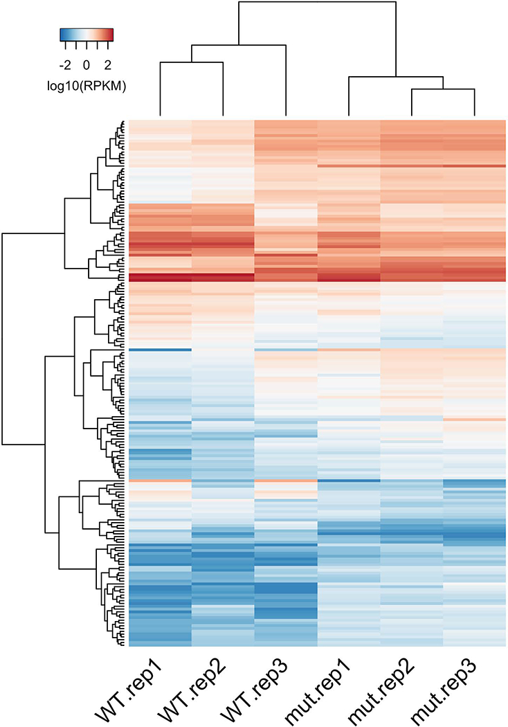
• 18. For a more detailed visualization of expression patterns, a heatmap of the expression values of differentially expressed genes across all individual samples can be generated (Fig. 3). To highlight grouping among samples and recurrent expression patterns among genes, heatmaps are typically clustered both by columns (samples) and rows (genes), often using a hierarchical clustering method. The degree of inferred similarity between individual samples and between individual genes can be represented as dendrograms of columns and rows, respectively (Fig. 3). Inspection of these heatmaps can provide more detailed information about similarities and differences of expression patterns between samples and between conditions, as well as about groups of genes whose expression behaves in a similar way. Below is an example of R commands using the R package gplots to produce an expression heatmap, as a graphic PNG file, from the table of differentially expressed genes produced at step 16.

  library(gplots)
  de.genes = rownames(de.gene.logFC)
  rpkm = rpkm(cds,gene.length)
  de.gene.RPKM.mtx = log10(rpkm[de.genes,]+0.1)
  colfunc <- colorRampPalette(brewer.pal(9,”Blues”))
  png(“DE.gene.heatmap.png”,5,7,units = “in”,res=300) heatmap.2(de.gene.RPKM.mtx,col=colfunc(100),trace=“none”,labRow=““,cexRow=1,cexCol=1.5,lhei=c(1,5), lwid=c(1, 3), density.info=“none”,margins = c(5,1),srtCol=45,key.title = ““,key.xlab = “logRPKM”)
  dev.off()

  These commands generate the file DE.gene.heatmap.png that contains the expression heatmap with samples and genes clustered using a basic hierarchical clustering method (Fig. 3). Since this clustering is non-supervised, the grouping of samples by the patterns of gene expression can serve as an additional verification of consistency between experimental replicates and provide a more detailed view of inconsistencies between potential outlier samples and the rest of the group (sample WT.rep3 in Fig. 3), in addition to a more general view of samples as points in the MDS or PCA plots (step 14). Most importantly, these heatmaps provide a detailed visual summary of expression differences between compared experimental conditions at the level of individual genes and groups of genes.

• 19. The tables of differentially expressed genes (Table 4) can be further inspected manually and analyzed computationally. Among various ways that the data can be further analyzed, the list of differentially expressed genes can be used to detect the enrichment of functional gene sets using a variety of computational methods such as DAVID (Huang et al., 2018) (http://david.ncifcrf.gov) or EnrichR (Kuleshov et al., 2016) (http://amp.pharm.mssm.edu/Enrichr/), among many others. As an alternative approach, the enrichment of functional gene sets can also be analyzed using the full tables of expression and fold change values across all genes in the genome (product of step 15), for example by submitting these ranked whole-genome tables to the GSEA tool (Subramanian et al., 2005).

Figure 1.

Example of MDS plot of six RNA-seq samples. Each sample is shown as a two-dimensional point represented by text (sample name) and colored by group (condition). In this particular case, the group of three biological replicates from mutant samples (mut, shown in red) is well separated from the group of three biological replicates from wild-type samples (WT, shown in black). In the WT group, replicate 3 (WT.rep3) is separated from other replicates of the same group and may be a potential outlier.

Figure 2.

Example of a Volcano plot. Each gene is represented as a point in the space of absolute difference in expression value between two compared groups of replicates (log2 of fold change, logFC) as the x axis and the statistical significance of this difference (-log10 of FDR or P-value) as the y-axis. The plot has a characteristic shape reflecting a general relationship between fold change and statistical significance. The overall distribution of points is usually symmetrical between up-regulated genes (points to the right of x=0) and down-regulated genes (points to the left of x=0), with the majority of points located near the origin, which corresponds to small and statistically insignificant differences. Differentially expressed genes (highlighted in red) are defined here by the cutoffs of 2-fold change (logFC > 1 or logFC < −1) and statistical significance < 0.01.

Figure 3.

Heatmap of expression values of differentially expressed genes across individual samples. Clustering of expression patterns of samples (columns) and genes (rows) is represented by the dendrograms on top and on the left, respectively. Color indicates expression value (log10 of RPKM).

Table 4.

The table of differentially expressed genes (example)

Gene Name	logFC	logCPM	PValue	FDR
Rbmxl2	−12.2	2.5	3.2E-72	3.7E-70
Dppa3	−12.2	2.5	3.7E-72	4.3E-70
Utf1	−12.1	2.5	2.8E-71	3.1E-69
Neto1	11.9	2.3	1.0E-67	9.9E-66
Elf3	−11.1	1.5	1.1E-54	6.1E-53
Vrtn	−11.1	1.5	4.4E-54	2.3E-52
Tdh	−11.1	1.5	1.8E-53	9.2E-52
Fgf4	−11.0	4.5	6.6E-106	4.9E-103
EU599041	−10.9	1.3	1.6E-51	7.5E-50

For each identified gene, the table indicates gene name (column 1), log2 fold change of absolute expression (logFC), average expression (CPM) value across all compared samples in the log2 scale (logCPM), P-value, and false discovery rate (FDR) as an estimate of statistical significance of differential expression.

COMMENTARY

Background Information

The STAR aligner described in this UNIT and similar methods represent an approach to mapping reads to a whole genome as well as attempting to identify splicing events across non-contiguous exons and UTRs whose genomic coordinates come from the reference genome annotation supplied by the user. This is a computationally intensive but comprehensive and precise whole-genome approach to mapping. Another example of a similar but less computationally intensive approach is the BWA-MEM algorithm of the popular BWA aligner, which is able to map a chimeric sequencing read that is comprised of parts from separate regions of the genome (Li and Durbin, 2009). There are also various methods that can be used as alternatives to the HTSeq package at the stage of quantitating reads mapped to each transcript, for example RSEM (Li and Dewey, 2011).

A few alternative computational methods (Roberts and Pachter, 2013, Patro et al, 2014, Bray et al, 2016, Patro et al, 2017) bypass the stage of precise mapping of a read to the reference transcriptome and proceed directly to quantification of transcript abundance using more indirect but faster algorithmic approaches, for example quantitating the representation of short k-mer strings within the reads and the reference transcripts. Many of these methods are focused on assigning reads to the fully spliced mRNA (cDNA) sequences, which additionally increases speed by concentrating on a small fraction of the total genome, albeit at the potential price of being confined to identifying only the transcript isoforms included in the reference cDNA set. These approaches are faster and more lightweight than traditional aligners. As an example, Salmon (Patro et al, 2017) is a relatively fast and user-friendly method for both mapping and quantitation of RNA-seq reads and may be attractive especially for an entry-level user.

The edgeR package used in this pipeline is conceptually similar to other popular tools for statistical analysis of differential expression, DEseq (Anders et al., 2012), DESeq2 (Love et al. 2014), DEXseq (Li et al., 2015).

Critical Parameters and Troubleshooting

Quality assessment is essential to ensure robust and reproducible results. Although the quality and relevance of the intermediate results should be assessed throughout the workflow, two steps are the most important and informative. Picard or similar analytical tools produce metrics that indicate the quality of RNA extraction, library construction, and, to a lesser extent, sequencing (step 5). A high-quality RNA-seq library corresponds to a > 90% read mapping rate, a high level of “usable” nucleotide bases, and contains less than 5% ribosomal RNA reads. PCR over-amplification can be evaluated by the duplication rate and, in more detail, by visual examination of BAM files as tracks in a genome viewer.

At the step of differential expression analysis, sample-centric MDS plots can reveal potential outlier samples that may bias downstream identification of differentially expressed genes. Gene-centric Volcano or other conceptually similar plots can help verify the general distribution and relationships between metrics of differential expression for individual genes.

Two important parameters for calling differentially expressed genes are the cutoffs of fold change and statistical significance (typically FDR), which are most often set to 2-fold and 0.01 or 0.05, respectively. In a typical RNA-seq experiment in mammalian cells or tissues, one would usually expect to identify between a few hundred and a few thousand differentially expressed genes, depending on the experimental design.

Anticipated Results

This protocol is expected to generate a table of expression values for all genes in all samples, a list of candidate differentially expressed genes between compared sample groups, an MDS plot with relative positioning of samples as points in multi-dimensional space, and a volcano plot that shows expression fold changes and their statistical significance for individual genes. At the earlier stages, this protocol generates a table of quality metrics for input RNA-seq datasets.

Time Considerations

The timing depends on the number of samples, number of reads per sample, number of comparisons between sample groups, and the available computational resources. Minimal hardware requirements for a basic analysis in a mammalian genome include Unix, Linux or MacOS operating system, 30 GB of RAM, and 50 GB of disk space for storing reference genome and output files. Alignment of sequencing reads typically takes the largest amount of time. As a very rough estimate, STAR can align 10–100 million reads per hour to a mammalian reference genome. Picard, HTseq, edgeR analyses and data inspection may take a few hours each. After installation of all required packages, the full comparison of two sample groups with three biological replicates in each group usually takes 1–2 days.

Literature Cited

- Anders S, Pyl PT and Huber W, 2015. HTSeq a Python framework to work with high-throughput sequencing data. Bioinformatics, 31(2), pp.166–169. [DOI] [PMC free article] [PubMed] [Google Scholar]
- Anders S and Huber W, 2012. Differential expression of RNA-Seq data at the gene level-the DESeq package Heidelberg, Germany: European Molecular Biology Laboratory (EMBL). [Google Scholar]
- Bray NL, Pimentel H, Melsted P, Pachter L., 2016. Near-optimal probabilistic RNA-seq quantification. Nature Biotechnology 34, p. 525–527. [DOI] [PubMed] [Google Scholar]
- DeLuca DS, Levin JZ, Sivachenko A, Fennell T, Nazaire MD, Williams C, Reich M, Winckler W, Getz G., 2012. RNA-SeQC: RNA-seq metrics for quality control and process optimization. Bioinformatics 28:1530–2. [DOI] [PMC free article] [PubMed] [Google Scholar]
- Dobin A, Davis CA, Schlesinger F, Drenkow J, Zaleski C, Jha S, Batut P, Chaisson M and Gingeras TR, 2013. STAR: ultrafast universal RNA-seq aligner. Bioinformatics, 29(1), pp.15–21. [DOI] [PMC free article] [PubMed] [Google Scholar]
- Dobin A and Gingeras TR, 2015. Mapping RNA‐seq reads with STAR. Current Protocols in Bioinformatics, pp.11–14. [DOI] [PMC free article] [PubMed] [Google Scholar]
- Love MI, Huber W, Anders S (2014). “Moderated estimation of fold change and dispersion for RNA-seq data with DESeq2.” Genome Biology, 15, 550. [DOI] [PMC free article] [PubMed] [Google Scholar]
- Robinson MD, McCarthy DJ and Smyth GK, 2010. edgeR: a Bioconductor package for differential expression analysis of digital gene expression data. Bioinformatics, 26(1), pp.139–140. [DOI] [PMC free article] [PubMed] [Google Scholar]
- Huang DW, Sherman BT and Lempicki RA, 2008. Systematic and integrative analysis of large gene lists using DAVID bioinformatics resources. Nature protocols, 4(1), p.44. [DOI] [PubMed] [Google Scholar]
- Kuleshov MV, Jones MR, Rouillard AD, Fernandez NF, Duan Q, Wang Z, Koplev S, Jenkins SL, Jagodnik KM, Lachmann A and McDermott MG, 2016. Enrichr: a comprehensive gene set enrichment analysis web server 2016 update. Nucleic Acids Research, 44(W1), pp.W90–W97. [DOI] [PMC free article] [PubMed] [Google Scholar]
- Li B and Dewey CN, 2011. RSEM: accurate transcript quantification from RNA-Seq data with or without a reference genome. BMC bioinformatics, 12(1), p.323. [DOI] [PMC free article] [PubMed] [Google Scholar]
- Li H and Durbin R, 2009. Fast and accurate short read alignment with Burrows-Wheeler transform. Bioinformatics, 25(14), pp.1754–1760. [DOI] [PMC free article] [PubMed] [Google Scholar]
- Li H, Handsaker B, Wysoker A, Fennell T, Ruan J, Homer N, Marth G, Abecasis G, Durbin R; 1000 Genome Project Data Processing Subgroup, 2009. The Sequence Alignment/Map format and SAMtools. Bioinformatics 25:2078–9. [DOI] [PMC free article] [PubMed] [Google Scholar]
- Li Y, Rao X, Mattox WW, Amos CI and Liu B, 2015. RNA-seq analysis of differential splice junction usage and intron retentions by DEXSeq. PloS one, 10(9), p.e0136653. [DOI] [PMC free article] [PubMed] [Google Scholar]
- Okonechnikov K, Conesa A, García-Alcalde F, 2016. Qualimap 2: advanced multi-sample quality control for high-throughput sequencing data. Bioinformatics 32:292–4. [DOI] [PMC free article] [PubMed] [Google Scholar]
- Patro R, Duggal G, Love MI, Irizarry RA, & Kingsford C, 2017. Salmon provides fast and bias-aware quantification of transcript expression. Nature Methods 14, p. 417–419. [DOI] [PMC free article] [PubMed] [Google Scholar]
- Patro R, Mount SM, Kingsford C., 2014. Sailfish enables alignment-free isoform quantification from RNA-seq reads using lightweight algorithms. Nature Biotechnology 32, p. 462–464. [DOI] [PMC free article] [PubMed] [Google Scholar]
- Roberts A and Pachter L, 2013. Streaming fragment assignment for real-time analysis of sequencing experiments. Nature methods, 10(1), p.71. [DOI] [PMC free article] [PubMed] [Google Scholar]
- Robinson JT, Thorvaldsdóttir H, Winckler W, Guttman M, Lander ES, Getz G and Mesirov JP, 2011. Integrative genomics viewer. Nature Biotechnology, 29(1), p.24. [DOI] [PMC free article] [PubMed] [Google Scholar]
- Subramanian A, Tamayo P, Mootha VK, Mukherjee S, Ebert BL, Gillette MA, Paulovich A, Pomeroy SL, Golub TR, Lander ES and Mesirov JP, 2005. Gene set enrichment analysis: a knowledge-based approach for interpreting genome-wide expression profiles. Proceedings of the National Academy of Sciences, 102(43), pp.15545–15550. [DOI] [PMC free article] [PubMed] [Google Scholar]
- Trapnell C, Hendrickson DG, Sauvageau M, Goff L, Rinn JL, Pachter L., 2013. Differential analysis of gene regulation at transcript resolution with RNA-seq. Nature Biotechnology 31(1):46–53. [DOI] [PMC free article] [PubMed] [Google Scholar]
- Zerbino DR, Achuthan P, Akanni W, Amode MR, Barrell D, Bhai J,& Gil L. (2017). Ensembl 2018. Nucleic Acids Research, 46(D1), D754–D761. [DOI] [PMC free article] [PubMed] [Google Scholar]