Strategies for processing and quality control of Illumina genotyping arrays

Abstract

Illumina genotyping arrays have powered thousands of large-scale genome-wide association studies over the past decade. Yet, because of the tremendous volume and complicated genetic assumptions of Illumina genotyping data, processing and quality control (QC) of these data remain a challenge. Thorough QC ensures the accurate identification of single-nucleotide polymorphisms and is required for the correct interpretation of genetic association results. By processing genotyping data on > 100 000 subjects from >10 major Illumina genotyping arrays, we have accumulated extensive experience in handling some of the most peculiar scenarios related to the processing and QC of Illumina genotyping data. Here, we describe strategies for processing Illumina genotyping data from the raw data to an analysis ready format, and we elaborate on the necessary QC procedures required at each processing step. High-quality Illumina genotyping data sets can be obtained by following our detailed QC strategies.

Introduction

High-throughput genomic technology has revolutionized the landscape of biomedical research. One of the early representative high-throughput genomic technologies is the microarray, which was the dominate technology for gene expression quantification and genotyping. However, since the introduction of high-throughput sequencing (HTS), the application of gene expression quantification by microarray has gradually diminished [1–5]. HTS-based RNA sequencing offers competitive prices and numerous analytical advantages, such as the ability to detect structural variants and novel transcripts [6]. However, the decline of the gene expression microarray has coincided with a rising market for genotyping arrays thanks to new strategies and products set forth by Illumina.

Genotyping microarrays are also referred to as single-nucleotide polymorphism (SNP) arrays, and have been the tool of choice for genome-wide association studies (GWASs) for the past 15 years. Illumina has a long history of designing and producing genotyping arrays, with many of them powering important GWAS. One of Illumina’s newest series of products is the exome array with ∼240 000 SNPs, which, depending on the version, focuses on exonic variants, with an additional 24.8% of the SNPs from the GWAS catalog [7]. With a substantial portion (68%) of the SNPs on exome arrays being rare, with minor allele frequency (MAF) <1%, special protocols [8] have been developed to process and quality control (QC) these data. The latest Illumina genotyping array is the Infinium Expanded Multi-Ethnic Genotyping Array (MEGA^EX), which contains >2 million SNPs and covers 65.7% of GWAS catalog SNPs.

The most attractive feature of these new Illumina arrays is their affordability, with prices at $55–$70 per array. Compared with the cost of $600–$700 of exome sequencing per sample, the exome chip offers a much more fiscally reasonable alternative for conducting large-scale GWASs. The exome arrays have quickly become popular and power many high-profile genetic and association studies [9–11]. With the affordable price, excellent SNP content and customizability, the MEGA^EX array is poised to become the next popular genotyping platform for large-scale genetic association studies.

The processing and QC of Illumina genotyping arrays can be divided into two major stages based on the primary tools used: GenomeStudio and PLINK [12]. GenomeStudio is an Illumina-designed software that processes their raw genomic data. There are no alternative methods for processing Illumina genotyping array currently. The Genotyping Module of GenomeStudio processes the Illumina genotyping array from raw data to PLINK format, which is the standard format for storing genotyping data. Quality control has always been a major component in high-throughput genomic data processing, and thorough QC at multiple steps of data processing is necessary to ensure data integrity [13–16]. Various QC procedures can be performed at both the GenomeStudio and PLINK level. Here, we will describe detailed strategies for the processing and QC of Illumina genotyping arrays from multiple perspectives.

GenomeStudio processing

Data loading

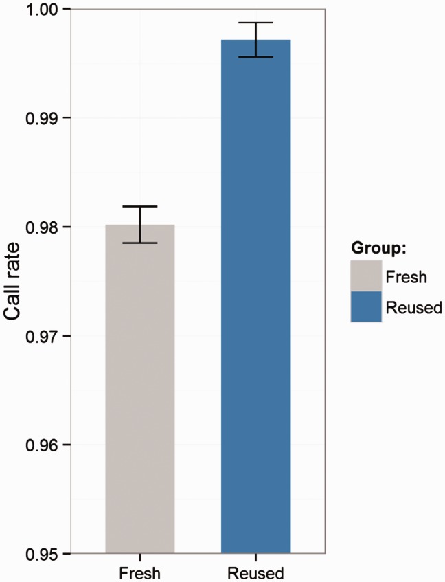
The first step of analyzing Illumina genotyping data is to load the raw data into GenomeStudio, which can be a tedious process for large projects with hundreds of sample sheets. Generally, each sample sheet can contain up to 96 samples (96 samples per plate). GenomeStudio only permits one sample sheet to be loaded at a time, which is vastly inefficient. Instead, multiple sample sheets can be merged into one sheet to load all samples at once. While loading the data, an option is given of including a previous available cluster file. The cluster file can be exported from other genotyping projects of the same array design that has already been subjected to rigorous QC. Using a cluster file that has already been quality controlled significantly reduces the chance of miss-clustering and improves the call rate of samples. This improvement is of particular importance for rare variants, which are often included on the latest generations of the genotyping platforms. An example of the benefit for using a QC cluster file is presented in Figure 1.

Figure 1.

Improvement through use of a previous clustering file. In this example, a cluster file was exported from a genotyping project using the MEGA^EX array of 7300 subjects after thorough QC. A new genotyping project using the same array on 64 subjects was clustered with and without the exported cluster file from the previous 7300 subjects. We observed an average of 1.70% (range: 1.34–1.90%) call rate increase per sample when clustering with a previously quality controlled cluster file. This evidence proves that using a well quality controlled cluster file can significantly (paired t-test P-value <0.0001) improve the call rate of samples.

Clustering

The design of a genotyping array is based on the concept of hybridization technology. To detect the two alleles of a SNP, two probes (oligonucleotides) are synthesized to capture each of the two alleles (alleles A and B) for the SNP. A SNP can be represented as AA, AB and BB genotypes. The fluorescently labeled target sequences created from source samples bind to the two probe sequences and generate a signal that depends on the hybridization conditions. The level of fluorescent intensity of each probe represents the signal strength for each allele. After measuring fluorescent levels of the two probes from multiple samples, a cluster algorithm is applied to the fluorescent levels to form a cluster that distinguishes samples into AA, AB and BB clusters (Figure 2A). The cluster can also be viewed after a polar transformation of the A and B intensity for better clarity (Figure 2B).

Figure 2.

(A) The cluster plot presented in Cartesian coordinates. The x-axis is the normalized intensity for allele A. The y-axis is the normalized intensity for allele B. (B) The same cluster plot presented in polar coordinates. The x-axis is the normalized θ, which is computed as$\mathrm{\theta }=\frac{2}{\pi }\mathrm{a}\mathrm{r}\mathrm{c}\mathrm{t}\mathrm{a}\mathrm{n}\left(\frac{1}{AB}\right)$. The y-axis is the normalized$R$, which is computed as $R=A+B$. In both plots, the red cluster (Left in A and Right in B) denotes the AA genotype, the purple cluster (middle) denotes the AB genotype and the blue cluster (Left in A and Right in B) denotes the BB cluster. The samples in between clusters (black) were not assigned a genotype. A colour version of this figure is available at BIB online: https://academic.oup.com/bib.

After loading the raw data into GenomeStudio, the clustering of intensities for all SNPs is performed. The next step is to filter out low-quality samples. For large studies containing thousands of subjects, we expect around a 1–2% sample failure rate [8]. The best parameter to measure overall sample quality is the call rate, which measures the percentage of SNPs with genotype calls for a sample. Different genotyping arrays might have different call rate standards, yet the commonly used call rate standard is 95–98% [8]. Any sample below the call rate standard should be excluded from further analysis. Inside GenomeStudio, a useful option for displaying the clusters is to hide the excluded samples, which can substantially improve the cluster clarity (Figure 3).

Figure 3.

(A) An example of a SNP cluster with plot with samples that should be removed because of low sample quality. (B) The same SNP with the poor-quality samples removed. The cluster became much clearer. A colour version of this figure is available at BIB online: https://academic.oup.com/bib.

Manual re-clustering

The cluster algorithm used in GenomeStudio’s genotyping module is called GenTrain. The exact implementation of the algorithm has not been disclosed by Illumina. The algorithm works well on a majority of the SNPs on any Illumina genotyping array. However, up to 5% of all SNPs may be miss-clustered, meaning that the AA, AB and BB clusters are not correctly identified [8]. In this case, the software operator can manually fix these clusters. There are several important QC measurements for SNP calling within GenomeStudio that can aid in identifying the SNPs that might need to be manually re-clustered. Again, the increase in the number of rare variants included in the design of the latest generation of genotyping platforms makes it imperative that these QC measurements are used, as these rare variants are the most likely to fail automatic clustering.

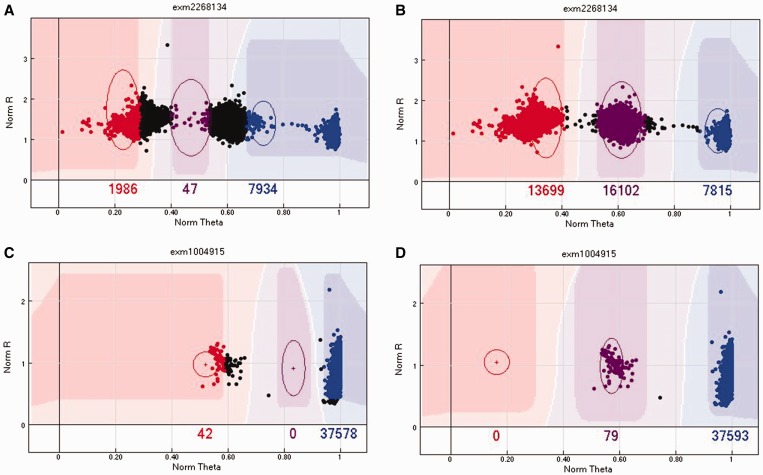
The most important QC parameter is the GenTrain score. The GenTrain score is computed from the GenTrain 2.0 clustering algorithm. It is a measurement of SNP calling quality, ranging from 0 to 1, with higher value meaning better quality. An example of a GenTrain score is given in Figure 4. The second most important QC parameter is the cluster separation score, which measures how well the AA, AB and BB clusters are separated. The cluster separation score also ranges from 0 to 1, with higher meaning better (more separation). An example of a cluster separation score is given in Figure 4. The third most important QC parameter is call frequency, which measures the percentage of samples with successful calls for that SNP. The call frequency also ranges from 0 to 1, with higher meaning more samples have successful calls for this SNP. These three scores are often positively correlated, but they also identify unique scenarios to which only one of the three measures may be sensitive. Therefore, to determine whether manual re-clustering is needed, it is best to sort the SNPs by each of the three QC parameters, from small to large, and go through the SNPs with the lowest scores on any of the three measures.

Figure 4.

(A) An example of a SNP with low GenTrain score (0.42). (B) By manually realigning the cluster positions, the cluster becomes much clearer and the GenTrain score improves to 0.8. (C) An example of miss-cluster by the GenTrain algorithm, with a cluster separation score of 0.65. (D) The same SNP was re-clustered by manually realigning the cluster positions, and the cluster separation score increased to 1. A colour version of this figure is available at BIB online: https://academic.oup.com/bib.

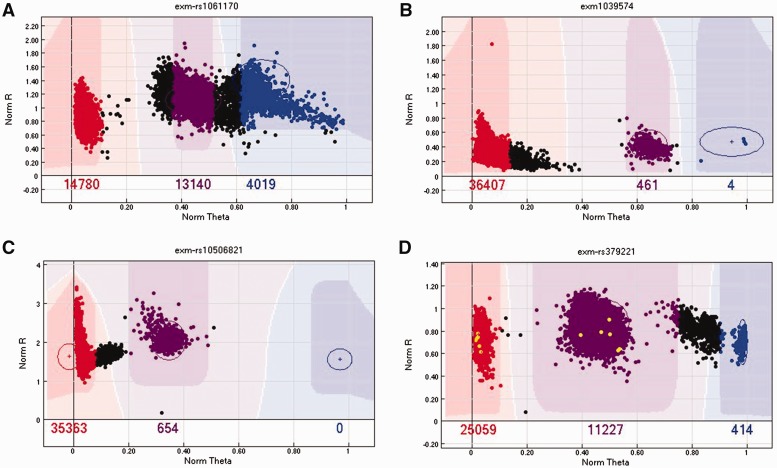
Peculiar cluster scenarios can arise. For example, homozygous and heterozygous clusters can be close, making the clusters hard to separate (Figure 5A). Sometimes, the AA or BB cluster may have a long tail (Figure 5B), or a strange extension (Figure 5C). Occasionally, four clusters can be observed instead of three (Figure 5D). In all of these scenarios, it is better to take the conservative approach of either removing the SNP or just the samples that appeared outside the normal cluster pattern, for example in the long tail.

Figure 5.

(A) An example of a SNP with presumed AB and BB clusters closely connected. In this scenario, either remove the SNP (preferred) or remove the samples between the clusters. (B) An example of a SNP with a long tail in the AA cluster. We recommend removing the samples of the tail to be conservative. (C) An example of a SNP with a strange extension or tail in the AA cluster. The exact cause of this pattern is unknown. We recommend either removing the SNP or removing the samples in the extension. (D) An example of a SNP with four visible clusters that does not make biological sense. We recommend removing this SNP. A colour version of this figure is available at BIB online: https://academic.oup.com/bib.

Repeat samples and Mendelian errors

All large-scale genotyping studies contain control samples to assess quality. The control samples are either repeats of samples or family trio (father, mother and child) samples from HapMap [17]. GenomeStudio assesses the repeat error from repeated samples and the Mendelian error from family trio samples. Repeat errors occur when genotypes of the same SNP are different between repeated samples. Mendelian errors are instances where an offspring’s germ line alleles are not obtained through Mendelian inheritance from each parent. For example, for a SNP, the mother has [A/A] genotype, the father has [A/A] genotype and the child has [A/C] genotype. The C allele is considered a Mendelian error. In GenomeStudio, Mendelian errors are referred to as parent–parent–child (PPC) errors, or parent–child (PC) errors when only one parent is available. While Mendelian errors may be true de novo mutations, in general, they indicate genotyping problems with that SNP. SNPs with excessive (>10) repeat or Mendelian errors should be considered for removal.

Sex chromosomes and mitochondria

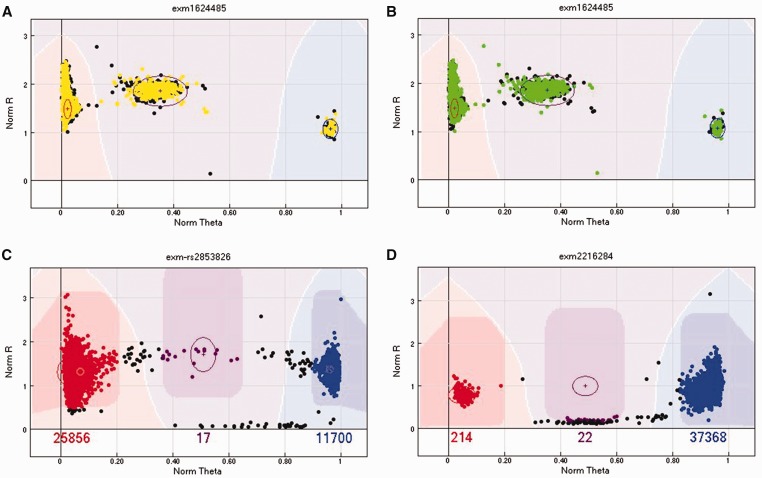
Chromosomes 1–22 are diploid, meaning they have two alleles for each SNP. There are also two sex chromosomes: X and Y. Females have two copies of X, making them diploid, while males have only one copy of X and one copy of Y. The quality assessment of SNPs on chromosome X and Y should be stratified by sex. A further complication is that on sex chromosomes, there are many pseudoautosomal regions (PAR), which are homologous regions that result from the pairing and recombining of chromosome X and Y during meiosis. SNPs on PARs are usually annotated as chromosome XY. However, in some arrays, the PAR SNPs are labeled simply as SNPs on Chromosome X. Thus far, there have been three PARs identified [18, 19]. SNPs in PARs should be treated as diploid, even in males, instead of as sex chromosomes. Examples of problematic SNPs on sex chromosomes are given in Figure 6.

Figure 6.

(A) An example of a problematic SNP on chromosome X. The male subjects are presented in yellow (Gray when printing in grayscale), and they should not appear in the AB cluster because males are haploid on chromosome X. (B) An example of a problematic SNP on chromosome Y. The female subjects are presented in green (Gray when printing in grayscale), and they should not be included in any cluster because females do not have chromosome Y. (C) An example of an mtDNA SNP. The AB cluster indicates the presence of heteroplasmy in numerous samples at this site. (D) An example of an mtDNA SNP where the AB cluster included a few samples with low R values by mistake. This problem can be resolved by moving the AB cluster slightly up. A colour version of this figure is available at BIB online: https://academic.oup.com/bib.

Mitochondria contain a maternally inherited haploid genome, mitochondrial DNA (mtDNA). At any given position on the mitochondrial genome, there should only be one allele. This characteristic will theoretically make any SNP on a mitochondrion appear to be either the AA or BB genotype. This is true for a majority of samples and mtDNA SNPs. However, mammalian cells can contain many mitochondria, and each mitochondrion can contain up to 10 copies of mtDNA [20]. Therefore, mtDNA is often heteroplasmic (containing both normal and mutant copies of mtDNA) [21, 22]. The characteristic of heteroplasmy can be seen in the cluster plot as an AB cluster [23]. The appearance of the AB cluster for mtDNA SNPs should be rare, with overwhelming representation of the AB cluster potentially indicating problematic SNPs. Examples of heteroplasmic SNPs on mitochondria are given in Figure 6. As with the sex chromosome, the quality of mtDNA SNPs should be assessed separately from the autosomal SNPs. However, unlike the sex chromosomes, it is not necessary to assess mtDNA SNP quality separately in males and females.

Rare SNPs

SNPs with MAF <1% can be problematic to cluster. The standard clustering algorithms were designed with common SNPs in mind. The GenTrain cluster algorithm often fails to identify low-frequency clusters, thus undercounting rare SNPs. To identify such SNPs, we can apply the following filters inside GenomeStudio: First, select the SNPs with MAF < 1%, select the SNPs with call frequency <0.999 and then select the SNPs with AB frequency <0.001. The call frequency filter will select SNPs with a small number of samples that are not called. The combination of these three filters will produce a list of SNPs with low or zero MAF. Some samples where these SNPs are uncalled are likely candidates to carry the minor allele of those rare SNPs, but were miss-clustered by the GenTrain algorithm.

There are two approaches of handling miss-clustered rare SNPs. The first approach involves using the program zCall [24], which can re-cluster the SNPs based on the GenomeStudio report file. Reports have shown that even though zCall can recover some miss-clustered rare SNPs, it can also introduce new false positives [8]. We recommend to only re-cluster the rare SNPs (MAF < 1%) to minimize the chance of additional false positives. The second approach is a brute force approach, meaning the manual review of all rare SNP candidates by selected filters.

PLINK quality control

GenomeStudio offers two major export formats: the GenomeStudio report and PLINK. As PLINK is the universal standard format for storing genotyping data, we will consider all of our remaining analyses based on the PLINK format. PLINK itself offers many useful QC functionalities, which we will discuss in detail.

Strand

One of the biggest weakness of the Illumina genotyping array design is Illumina’s definition of strand. As DNA is double-stranded, significant SNPs from GWAS need to be presented with their strand information to properly report the risk alleles. This unfortunately has not been a standard practice. The most intuitive definition of strand is to use the human genome reference as the forward strand. Defying logic, Illumina introduced a more convoluted definition of strand: top and bottom [25], which has caused great confusion with reference to the forward and reverse strand [26, 27]. While exporting genotyping data from GenomeStudio to a PLINK format file, an option can be selected to convert all SNPs to the forward strand. However, this ‘Forward Strand’ definition is either different from the conventional one or various bugs exist in the conversion algorithm, causing ∼1–1% of all SNPs to not be converted to the forward strand in the exported PLINK file on various Illumina genotyping arrays.

Various strategies can be applied to detect the strand of a SNP, such as comparing the calculated allele frequency with the allele frequency of a previously reported data set or to compare actual alleles with a reference population. However, when the allele frequency is near 50%, or the two alleles of the SNP are reverse complementary ([A/T] or [C/G]), these simple methods are not sufficient to identify the true strand of the SNP. A typical solution is to create strand flip files for converting the strand of the Illumina genotyping array. This type of approach [28, 29] requires the creation of a flip file for each version of the array, thus requiring frequent updates from the creator. The definite solution for strand ambiguity is to compare the probe sequence with the reference sequence, which has been implemented in StrandScript [30]. This type of approach is more future-proof because it is independent of the version of the Illumina genotyping array, as long as the probe sequences are accurately reported.

Sex and race

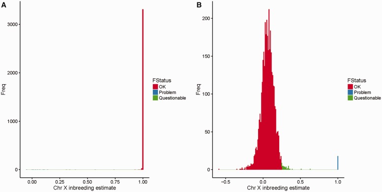
Sex and race are two self-reported clinical variables that are often subjected to error. Fortunately, sex and race can be determined through careful analysis of genotyping data. PLINK offers the functionality (–check-sex command) to estimate sex by computing inbreeding estimates using SNPs on chromosome X. The output of sex check is a text file of six columns. The fifth column is ‘Status’, which can be PROBLEM or OK. The sixth column contains the chromosome X inbreeding estimate. PLINK tends to overestimate the probability of sex mismatch. Instead, we recommend using the inbreeding estimate to assess sex of each sample. A male should have an inbreeding estimate for chromosome X >0.8. A female should have an inbreeding estimate <0.2. An example of sex check using PLINK is given in Figure 7.

Figure 7.

(A) An example of a histogram for the chromosome X inbreeding estimate computed by PLINK for males. (B) An example of a histogram for chromosome X inbreeding estimate computed by PLINK for females. The red color (Right in A and Left in B) indicates subjects with no obvious problems; the blue color (Left in A and Right in B) indicates samples with definitive problems that could be caused by blood transfusion, self-reporting or data entry errors. The green color (middle) indicates questionable samples, as they are outside the normal range for inbreeding estimates, but not strong enough to be defined as outliers. We recommend flagging these samples and deciding whether to exclude them based on other QC metrics. A colour version of this figure is available at BIB online: https://academic.oup.com/bib.

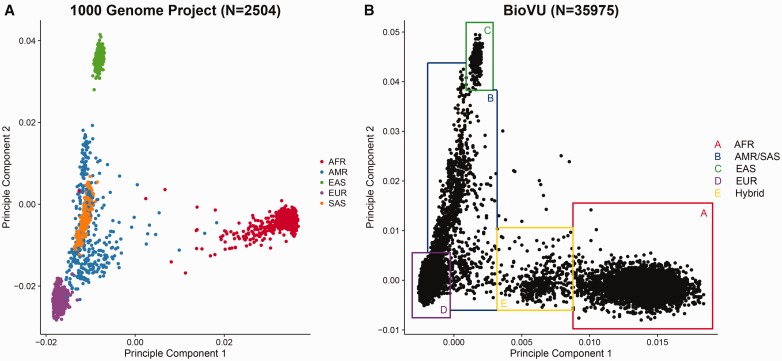
Race can be genetically determined by performing principle component (PC) analysis on ancestry informative markers (AIMs). AIMs are SNPs that exhibit substantially different allele frequencies between populations of different ethnicities. Each design of the Illumina genotyping array contains thousands of AIMs. The PC analysis can be performed using EIGENSTRAT [31]. PC1 and PC2 are considered practical surrogates of race, particularly for the US population. Genetic association studies often adjust for the first few PCs instead of actual race in their association models because the PCs can more accurately capture the intrinsic genetic difference even within a population ostensibly of the same race [32]. By plotting PC1 versus PC2, we can visualize the genetically determined race as positions on the scatter plot (Figure 8) and identify obvious outlier samples.

Figure 8.

(A) Scatter plot of PC1 versus PC2 computed by EIGENSTRAT from 1000G genotyping data. The samples are closely clustered by race. AFR=African ancestry populations, AMR=American Hispanics, EAS=East Asians, EUR=Caucasians, SAS=South Asians. Few outliers of race can be observed in the 1000 Genome Project data beyond that attributable to admixture. (B) Scatter plot of PC1 versus PC2 computed by EIGENSTRAT from Illumina exome array data. The shape of the clusters roughly resembles the one from the 1000 Genome Project. Instead of using self-reported race, we can determine the race by drawing boxes around clusters. Samples on the borders or outside the border of the boxes are ambiguous, as they could be results of blood transfusion or self-reporting or data entry errors. The Box E (yellow) indicates a group of likely first-generation mixed-race subjects between African and Caucasian ancestors. Such detailed ancestry information is usually not captured by self-report of race. This supports the rational that during association analysis, PCs should be used as surrogates of self-reported race. A colour version of this figure is available at BIB online: https://academic.oup.com/bib.

Hardy–Weinberg equilibrium

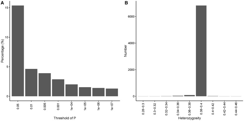
The Hardy–Weinberg equilibrium (HWE) principle states that allele frequencies in a population stay constant from one generation to the next without evolutionary influences. Departure from this equilibrium has been suggested as an indicator of potential genotyping errors, population stratification or even actual association to the trait under study [33, 34]. Large GWASs often test for deviation from HWE to detect genotyping errors in unrelated individuals [35, 36]. PLINK supports HWE tests with the ‘–hardy’ command, which generates a P-value to denote the significance of deviation from HWE. However, simply picking a cutoff P-value to filter out SNPs is not ideal. Many practical scenarios can cause significant P-values in HWE tests, such as selection, mutation, population stratification, immigration, etc. The P-value of a HWE test tends to contain many significant results by the standard P-value threshold P < 0.05. Different studies have adopted different HWE P-value standards anywhere from P < 0.001 to P < 10⁻⁷ [8, 37, 38]. These standards are usually arbitrary. In our opinion, only SNPs with extreme HWE P-values should be removed, and manual review of SNPs with low HWE P-values will prevent the exclusion of good SNPs.

The definition of HWE constrains it to a population; therefore, HWE tests should be applied to samples stratified by race. GenomeStudio offers the functionality for testing HWE. However, GenomeStudio cannot perform HWE tests stratified by race. Thus, if the genotyping data set contains samples of multiple races, PLINK is the better tool for examining HWE. Furthermore, if the genotyping data set is of a case-control study, the HWE test should be conducted only using the control samples because some diseases can cause deviation from HWE at disease-associated loci [39]. An example of the distribution of P-values for the HWE test is given in Figure 9A.

Figure 9.

(A) An example of the distribution of HWE P-values computed by PLINK from a genotyping data set of Caucasians obtained from the Illumina MEGA^EX array. Only SNPs with extreme P-values (right) should be candidates for removal. (B) An example of the distribution for heterozygosity computed by PLINK from a genotyping data set of Caucasians obtained from the Illumina MEGA^EX array. The majority of samples has heterozygosity values between 0.35 and 0.45. Only samples with extreme heterozygosity values are candidates for removal. Note that the expected heterozygosity value can differ by race [40].

Heterozygosity

Computing the heterozygosity rate for a genotyping data set with a large number of SNPs and a homogeneous sample population can help identify problematic SNPs, as higher heterozygosity may indicate sample contamination and low heterozygosity may indicate inbreeding. The testing of heterozygosity can be achieved in PLINK using the ‘–het’ command. An example of heterozygosity ratio distribution is given in Figure 9B.

Relatedness

Large-scale genotyping projects can contain up to tens of thousands of subjects. Some of these subjects may be related genetically with no record to indicate this. In standard association analysis, independence of the subjects is always assumed. Thus, it is important to test if any of the subjects are related by computing identity by state distance between all possible pair-wise samples through estimating pair-wise identity by descent (IBD). PLINK computes proportion IBD through the ‘–genome’ command. The proportion IBD is a numerical value ranging from 0 to 1, where 0 denotes no genetic relationship, >0.125 indicates 3rd degree relatives (cousins, etc.), >0.25 indicates 2nd degree relatives (half siblings, uncle, aunt etc.), >0.5 indicates 1st degree relatives (full siblings, parent–offspring) and values near 1 indicate duplicated samples or monozygotic twins. Moreover, the relatedness check can help identify potentially cross-contaminated samples when one sample’s DNA is mixed up with multiple other samples. The cross-contaminated samples can be detected as one-to-many higher than normal proportions of IBD.

Genotyping consistency

A good genotyping study design always includes external control samples from HapMap [17], 1000 Genomes Project (1000G) control samples [41] or internal duplicated samples. Genotyping consistencies can be computed between publicly released genotype data, in-house genotype data for external control samples and between the genotype data of repeated samples. The genotype consistency can be computed as an overall consistency or as heterozygous consistency. The overall genotype consistency is defined as the number of consistent SNPs divided by the number of overlapping SNPs. The heterozygous genotype consistency is defined as the number of consistent heterozygous SNPs divided by the number of heterozygous SNPs within the overlapping region. The overall consistency tends to be inflated because a majority of the human genome is reference homozygous. Heterozygous genotype consistency is a more conservative measure. For a successfully conducted genotyping study, the heterozygous genotype consistency rate is expected to be >97%, and the overall consistency rate is expected to be >99%. Furthermore, on all Illumina genotyping arrays, there are duplicated SNPs. Consistency rate can be computed between the duplicated SNPs across all samples. Identification of the duplicated SNPs not only requires the identification of the SNPs that target the same genomic positions but also the confirmation that they try to capture the same alleles. Strand flipping might be necessary to determine truly duplicated SNPs. The expected consistency rate for duplicated SNPs is >99%.

Allele frequency

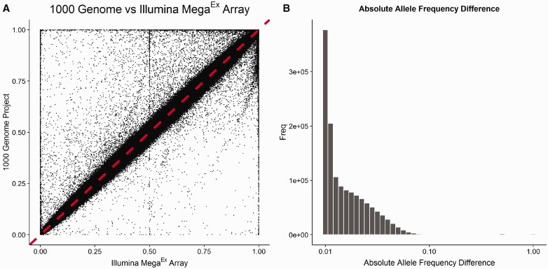
Another good QC measure is to compare the allele frequency of the locally genotyped data set with a publically available genotyping data set, such as the 1000G. As allele frequency is highly sensitive to race, the comparison should be stratified by race. An example of allele frequency comparison using MEGA^EX array data versus 1000G data is given in Figure 10. We expect to see a majority of the SNPs having a similar allele frequency as compared with 1000G data. The absolute difference of allele frequencies can be computed and sorted to identify the extreme allele frequency outliers, which may indicate problematic SNPs. Two examples of outliers are given in Figure 11. SNPs with an extreme allele frequency difference as compared with 1000G data should be filtered out. However, if large numbers of SNPs fail this comparison, this indicates that an improper 1000G reference set has been chosen which does not match the racial and ethnic makeup of your study.

Figure 10.

(A) An example of scatter plot of allele frequencies from the 1000 Genome Project versus allele frequencies from an Illumina MEGA^EX genotyping data set. All subjects are Caucasians. A majority (>99%) of the SNPs have similar allele frequencies. There are some outliers visible from the plot. (B) The distribution of allele frequency differences. To identify the obvious outliers by allele frequency, we can compute the absolute difference in allele frequencies and sort them from high to low.

Figure 11.

(A) The first example is for SNP rs144249066 in the MEGA^EX array. First, all subjects were called heterozygous [A/T], which strongly violates the HWE assumption. The HWE test had P<10⁻⁸ for this SNP in Caucasians, which means this SNP could be potentially filtered out by the HWE test. In 1000G data, this SNP was inferred as homozygous [A/A] for all Caucasians. Possible explanations are (1) the probe sequences were designed wrong or (2) they mapped to highly homologous regions. (B) The second example is for SNP rs113094557 on the MEGA^EX array. This SNP does not violate HWE, and the genotype type call is [G/G] for all Caucasians; however, the genotype call for all Caucasians in 1000G is [A/A]. The SNP has two probes designed to capture alleles A and G. As the two alleles are not reverse complementary, this could not be caused by a strand issue. The only plausible explanation is that the two alleles were switched or mislabeled by Illumina during design.

Batch effect

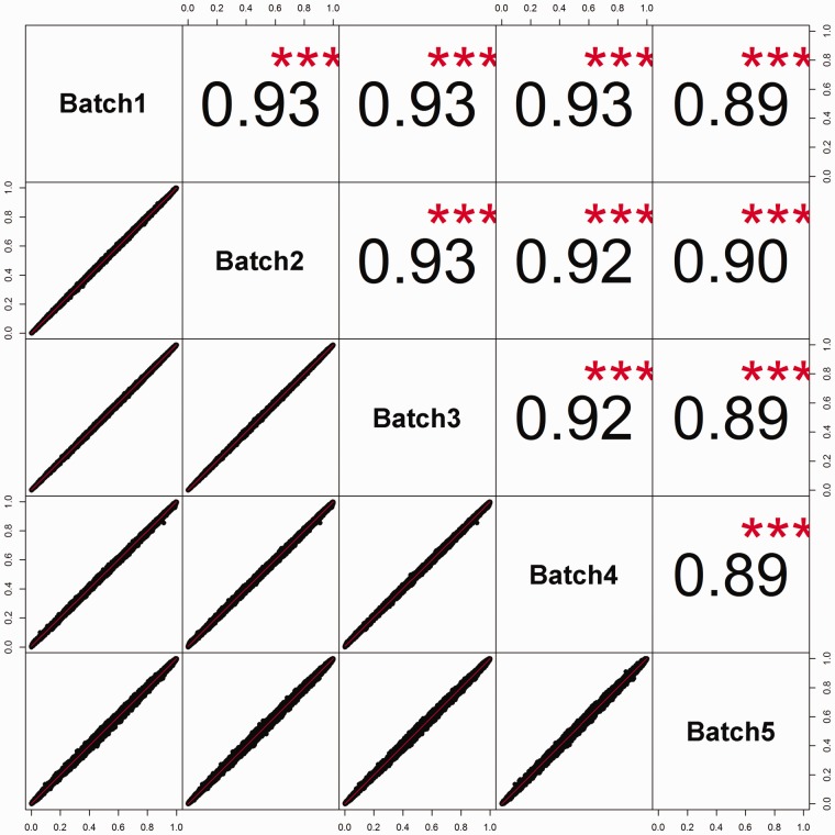
Batch effects are systematic variations in data caused by the processing of data in batches. Severe batch effects can yield misleading analysis results, especially for large data sets. For a large genotyping project, samples are usually prepared on a 96-well plate. Then, tens to hundreds of plates are genotyped in one time setting, which is considered a batch. The primary observable difference contributed to batch effect is the signal intensities because of laser calibration difference between batches. However, such variations in the laser strength usually are not severe enough to sway one genotype call to another one. Thus, it does not affect genotyping quality. However, this intensity variation can have an adverse effect on copy number variation (CNV) analysis because copy number is a continuous measurement inferred from the signal strength. Thus, copy number should be inferred by batch, and CNV analysis involving multiple batches should adjust for batch. To fully test whether other major batch effects exist, we can compute allele frequency consistencies between batches stratified by race. The correlation of allele frequencies between batches should be >0.9. Problematic SNPs can be identified by computing the absolute value of the allele frequency difference between batches and sort them from large to small. An example of an allele frequency consistency plot between multiple batches is given in Figure 12.

Figure 12.

An example of allele frequency comparisons among multiple batches. High correlation of the allele frequency between batches indicates no batch effect.

Computation time and memory requirements

Processing a large genotyping data set in GenomeStudio requires a powerful computer with extensive memory. To process a genotyping data set of 7350 subjects from the MEGA^EX array (2 million SNPs), we used a computer with the following specifications: Intel Xeon CPU E5-2699 v4 (22 cores) at 2.20 GHz, 396 GB memory, 64 bit Windows Server 2012. The amount of computational memory plays a significant role in the data processing speed and manual re-clustering speed.

When processing a large Illumina genotyping data set from raw data to a quality controlled PLINK genotyping data set, the majority of the time will be spent in GenomeStudio manually reviewing SNPs with problematic sample clusters and re-clustering them. The number of SNPs that can be manually reviewed is entirely arbitrary. The rule of manual reviewing is simple: the more SNPs manually reviewed, the better quality of the entire data set. Given the fact that the majority of SNPs are clustered correctly by the GenTrain algorithm (95–98%), approximately only 2–5% SNPs might be improved through manual reviewing. Current array density allows several million SNPs per chip, resulting in a huge amount of manually reviewable SNPs. Assuming it takes 30 s to manually review and re-cluster one SNP, manually reviewing the MEGA^EX array will take around 333–833 man-hours. Further, as the manual re-clustering occurs in GenomeStudio, parallel processing cannot be applied to save time. Thus, it is important to follow the recommendations to identify the most likely problematics SNPs, and manually review them. If time is greatly limited, we can focus manual review on SNPs with high priority. The priority of SNPs are arbitrary. For example, we can focus on the customized SNPs on the array first, as these are likely of special interest to the investigator, or we can focus on all SNPs that are in the GWAS catalog.

Discussion

Illumina genotyping arrays will remain a driving force in large-scale GWASs for years to come. We have described a series of techniques and QC strategies for processing Illumina genotyping arrays from raw data to an analysis-ready PLINK format file. The processing of Illumina genotyping arrays can be divided into two major sections: (1) inside GenomeStudio and (2) in PLINK format. The GenomeStudio section primarily deals with initial SNP clustering and manual re-clustering. The QC steps in PLINK primarily ensure data integrity through multiple rigorous tests based on genetic assumptions. There are currently two major genotyping array companies: Illumina and Affymetrix. The initial processing of data from Affymetrix genotyping arrays is different from that of Illumina’s. The strategies we have described in GenomeStudio would not work for Affymetrix genotyping arrays. However, once the Affymetrix genotyping arrays are converted to PLINK format, all of the strategies described for PLINK data can be applied. Furthermore, SNP data generated from HTS, even though more dense, are also genotyping data. Thus, some of the tests such as HWE, heterozygosity, etc. can also be used as QC measures. On the other hand, some QC metrics that have been proposed for HTS SNP data QC such as transition versus transversion ratio [40] can also be potentially applied to data generated from genotyping arrays.

We have outlined the major factors that can affect the quality of genotyping. There are some other unlikely factors that can also contribute to the quality of the data set. For example, blood transfusion is rare, but when it does happen, confusion for sample gender and race can arise. Also, Illumina’s SNP design is not perfect. Although rare, each of the Illumina genotyping arrays does contain hundreds to thousands of SNPs with potential design errors. Following the strategies we have described here will generate a genotyping data set of the highest quality.

Key Points

• Genotyping arrays provide an alternative mean for conducting large-scale GWASs.

• The Illumina’s genotyping arrays are popular, but the processing and QC of Illumina genotyping data require careful planning, meticulous QC.

• This manuscript provides all necessary processing and QC strategies to generate high-quality Illumina genotyping data set.

Shilin Zhao is a research fellow at the Department of Cancer Biology, Vanderbilt University. His research has been focused on bioinformatics research.

Wang Jing is a research fellow at Department of Cancer Biology, Vanderbilt University. She is a compositional biologist, specializing in RNA functions, and genotyping arrays.

David C. Samuels is an associate professor in the Department of Molecular Physics and Biology, Vanderbilt University. His research has been focused on mitochondria related topics.

Quanhu Sheng is a research assistant professor at the Department of Cancer Biology at Vanderbilt University. His research has been focused on small RNA sequencing and interpretation.

Yu Shyr is the Director of Center for Quantitative Sciences and professor of Biostatistics, Vanderbilt University. His research focuses on biostatistics and bioinformatics analysis of big data.

Yan Guo is an assistant professor at the Department of Cancer Biology, Vanderbilt University. He is the Technical Director of Bioinformatics for Vanderbilt Technologies for Advanced Genomics Analysis and Research Design.

References

- 1. Wang Z, Gerstein M, Snyder M.. RNA-Seq: a revolutionary tool for transcriptomics. Nat Rev Genet 2009;10:57–63. [DOI] [PMC free article] [PubMed] [Google Scholar]
- 2. Marioni JC, Mason CE, Mane SM, et al.RNA-seq: an assessment of technical reproducibility and comparison with gene expression arrays. Genome Res 2008;18:1509–17. [DOI] [PMC free article] [PubMed] [Google Scholar]
- 3. Asmann YW, Klee EW, Thompson EA, et al.3' tag digital gene expression profiling of human brain and universal reference RNA using Illumina genome analyzer. BMC Genomics 2009;10:531.. [DOI] [PMC free article] [PubMed] [Google Scholar]
- 4. Cloonan N, Forrest AR, Kolle G, et al.Stem cell transcriptome profiling via massive-scale mRNA sequencing. Nat Methods 2008;5:613–19. [DOI] [PubMed] [Google Scholar]
- 5. Guo Y, Sheng Q, Li J, et al.Large scale comparison of gene expression levels by microarrays and RNAseq using TCGA data. PLoS One 2013;8:e71462.. [DOI] [PMC free article] [PubMed] [Google Scholar]
- 6. Han L, Vickers KC, Samuels DC, et al.Alternative applications for distinct RNA sequencing strategies. Brief Bioinform 2015;16:629–39. [DOI] [PMC free article] [PubMed] [Google Scholar]
- 7. Hindorff LA, Sethupathy P, Junkins HA, et al.Potential etiologic and functional implications of genome-wide association loci for human diseases and traits. Proc Natl Acad Sci USA 2009;106:9362–7. [DOI] [PMC free article] [PubMed] [Google Scholar]
- 8. Guo Y, He J, Zhao S, et al.Illumina human exome genotyping array clustering and quality control. Nat Protoc 2014;9:2643–62. [DOI] [PMC free article] [PubMed] [Google Scholar]
- 9. Huyghe JR, Jackson AU, Fogarty MP, et al.Exome array analysis identifies new loci and low-frequency variants influencing insulin processing and secretion. Nat Genet 2013;45:197–201. [DOI] [PMC free article] [PubMed] [Google Scholar]
- 10. Szatkiewicz JP, Neale BM, O'Dushlaine C, et al.Detecting large copy number variants using exome genotyping arrays in a large Swedish schizophrenia sample. Mol Psychiatry 2013;18:1178–84. [DOI] [PMC free article] [PubMed] [Google Scholar]
- 11. Seddon JM, Yu Y, Miller EC, et al.Rare variants in CFI, C3 and C9 are associated with high risk of advanced age-related macular degeneration. Nat Genet 2013;45:1366–70. [DOI] [PMC free article] [PubMed] [Google Scholar]
- 12. Purcell S, Neale B, Todd-Brown K, et al.PLINK: a tool set for whole-genome association and population-based linkage analyses. Am J Hum Genet 2007;81:559–75. [DOI] [PMC free article] [PubMed] [Google Scholar]
- 13. Guo Y, Ye F, Sheng Q, et al.Three-stage quality control strategies for DNA re-sequencing data. Brief Bioinform 2014;15:879–89. [DOI] [PMC free article] [PubMed] [Google Scholar]
- 14. Guo Y, Zhao S, Ye F, et al.MultiRankSeq: multiperspective approach for RNAseq differential expression analysis and quality control. Biomed Res Int 2014;2014:248090. [DOI] [PMC free article] [PubMed] [Google Scholar]
- 15. Sheng Q, Vickers K, Zhao S, et al.Multi-perspective quality control of Illumina RNA sequencing data analysis. Brief Funct Genomics 2016, doi:10.1093/bfgp/elw035. [DOI] [PMC free article] [PubMed] [Google Scholar]
- 16. Guo Y, Zhao S, Sheng Q, et al.Multi-perspective quality control of Illumina exome sequencing data using QC3. Genomics 2014;103:323–8. [DOI] [PMC free article] [PubMed] [Google Scholar]
- 17. International HapMap Consortium. The international HapMap project. Nature 2003;426:789–96. [DOI] [PubMed] [Google Scholar]
- 18. Helena Mangs A, Morris BJ.. The human pseudoautosomal region (PAR): origin, function and future. Curr Genomics 2007;8:129–36. [DOI] [PMC free article] [PubMed] [Google Scholar]
- 19. Veerappa AM, Padakannaya P, Ramachandra NB.. Copy number variation-based polymorphism in a new pseudoautosomal region 3 (PAR3) of a human X-chromosome-transposed region (XTR) in the Y chromosome. Funct Integr Genomics 2013;13:285–93. [DOI] [PubMed] [Google Scholar]
- 20. Robin ED, Wong R.. Mitochondrial DNA molecules and virtual number of mitochondria per cell in mammalian cells. J Cell Physiol 1988;136:507–13. [DOI] [PubMed] [Google Scholar]
- 21. Ng SB, Buckingham KJ, Lee C, et al.Exome sequencing identifies the cause of a Mendelian disorder. Nat Genet 2010;42:30–5. [DOI] [PMC free article] [PubMed] [Google Scholar]
- 22. Durbin RM, Altshuler DL, Abecasis GR, et al.A map of human genome variation from population-scale sequencing. Nature 2010;467:1061–73. [DOI] [PMC free article] [PubMed] [Google Scholar]
- 23. Zhang P, Samuels DC, Zhao S, et al.Practicability of mitochondrial heteroplasmy detection through an Illumina genotyping array. Mitochondrion 2016;31:75–8. [DOI] [PubMed] [Google Scholar]
- 24. Goldstein JI, Crenshaw A, Carey J, et al.zCall: a rare variant caller for array-based genotyping: genetics and population analysis. Bioinformatics 2012;28:2543–5. [DOI] [PMC free article] [PubMed] [Google Scholar]
- 25. Illumina. “TOP/BOT” Strand and “A/B” Allele. http://res.illumina.com/documents/products/technotes/technote_topbot.pdf.
- 26. Nelson SC, Doheny KF, Laurie CC, Mirel DB. Is ‘forward’ the same as ‘plus’? … and other adventures in SNP allele nomenclature. Trends Genet 2012;28:361–3. [DOI] [PMC free article] [PubMed] [Google Scholar]
- 27. Nelson S, Zhao W, Smith J, Faul J. Health and retirement study: information for dbGaP users on annotation issues in the Illumina HumanOmni2.5-4v1_D manifest 2014, 2014. http://hrsonline.isr.umich.edu/sitedocs/genetics/ candidategene/HRS1 -2_dbGaPUserInfo_v3.pdf.
- 28. Robertson N. Genotyping chips strand and build files. http://www.well.ox.ac.uk/∼wrayner/strand/.
- 29. Wang K, Li MY, Bucan M.. Pathway-based approaches for analysis of genomewide association studies. Am J Hum Genet 2007;81:1278–83. [DOI] [PMC free article] [PubMed] [Google Scholar]
- 30. Wang J, Guo Y. StrandScript. https://github.com/seasky 002002/Strandscript.
- 31. Price AL, Patterson NJ, Plenge RM, et al.Principal components analysis corrects for stratification in genome-wide association studies. Nat Genet 2006;38:904–9. [DOI] [PubMed] [Google Scholar]
- 32. Samuels DC, Wang J, Ye F, et al.Heterozygosity ratio, a robust global genomic measure of autozygosity and its association with height and disease risk. Genetics 2016, doi:10.1534/genetics.116.189936. [DOI] [PMC free article] [PubMed] [Google Scholar]
- 33. Turner S, Armstrong LL, Bradford Y, et al.Quality control procedures for genome-wide association studies. Curr Protoc Hum Genet 2011;Chapter 1:Unit 1.19. [DOI] [PMC free article] [PubMed] [Google Scholar]
- 34. Wittke-Thompson JK, Pluzhnikov A, Cox NJ.. Rational inferences about departures from Hardy-Weinberg equilibrium. Am J Hum Genet 2005;76:967–86. [DOI] [PMC free article] [PubMed] [Google Scholar]
- 35. Gomes I, Collins A, Lonjou C, et al.Hardy-Weinberg quality control. Ann Hum Genet 1999;63:535–8. [DOI] [PubMed] [Google Scholar]
- 36. Hosking L, Lumsden S, Lewis K, et al.Detection of genotyping errors by Hardy-Weinberg equilibrium testing. Eur J Hum Genet 2004;12:395–9. [DOI] [PubMed] [Google Scholar]
- 37. Wellcome Trust Case Control Consortium. Genome-wide association study of 14,000 cases of seven common diseases and 3,000 shared controls. Nature 2007;447:661–78. [DOI] [PMC free article] [PubMed] [Google Scholar]
- 38. Meyre D, Delplanque J, Chevre JC, et al.Genome-wide association study for early-onset and morbid adult obesity identifies three new risk loci in European populations. Nat Genet 2009;41:157–9. [DOI] [PubMed] [Google Scholar]
- 39. Anderson CA, Pettersson FH, Clarke GM, et al.Data quality control in genetic case-control association studies. Nat Protoc 2010;5:1564–73. [DOI] [PMC free article] [PubMed] [Google Scholar]
- 40. Wang J, Raskin L, Samuels DC, et al.Genome measures used for quality control are dependent on gene function and ancestry. Bioinformatics 2015;31:318–23. [DOI] [PMC free article] [PubMed] [Google Scholar]
- 41. Abecasis GR, Auton A, Brooks LD, et al.An integrated map of genetic variation from 1,092 human genomes. Nature 2012;491:56–65. [DOI] [PMC free article] [PubMed] [Google Scholar]