Climate Migration at the Height and End of the Great Mexican Emigration Era

Abstract

Previous research has linked increasing climate-change-related variability to Mexico-US migration, but only under particular climatic/social conditions and periods of high irregular migration. Using the 2000 and 2010 Mexican censuses, we examine this environment-migration nexus across a broader set of socioecological contexts and during periods of both increasing (1995–1999) and declining (2005–2009) migration. Consistent with the notion that climate can “trap” populations in place, we find that frequent/severe bouts of hot or dry conditions are associated with lower US-bound migration from most of rural Mexico. However, we do find higher climate outmigration during episodes hot and dry climate, or out of places with lower vulnerability. Our comparisons across periods suggest that climate migration is affected by conditions in the U.S. in a similar or slightly weaker manner as other forms of migration are. Altogether, our findings suggest that rural Mexico is unlikely to push large numbers of international “climate refugees” and that climate migration is indeed sensitive to conditions in sending and destination areas.

Climate change has raised average temperatures across the world (IPCC 2013), largely through increases in atmospheric greenhouse gas emissions produced (within our outsourced) by the Global North (Bindoff 2013, Caney 2010). As part of these changes, rainfall has also declined in drier regions, including much of the plateau and highlands of Mexico (IPCC 2014), this study’s regional focus. With changing trends in temperature and precipitation, climatic variability is also expected to increase, which will be accompanied by more severe and frequent weather events (Hoerling and Kumar 2003, IPCC 2014, McGranahan et al. 2007). This outlook includes rapid-onset occurrences, like hurricanes or floods, as well as slower-onset episodes such as droughts, the focus of this paper and an important environmental stressor in much of Mexico (e.g., Ibarrarán et al. 2010).

Increasing temperatures and rainfall variability challenge local livelihoods and community development in large part because they also take place in the midst of important political-economic shifts (O’Brien and Leichenko 2000). In addition to rising exposure to environmental stress, individuals, families, and communities (in rural areas in particular) are increasingly sensitive to the changing climate owing not only to the cumulative effects of this exposure, but also to social and economic factors (see Adger 2006). Like many other developing nations, the Mexican political economy has been dramatically restructured over the last three decades. The country’s primary sectors were liberalized in the 1990s in several ways, including a reduction of public support for small-scale primary sector market activities (in both subsidies and credit availability, see De Janvry et al. 1995) and a gradual but complete opening of domestic agricultural markets under the North American Free Trade Agreement (Zepeda et al. 2009). Not unexpectedly, these structural shifts weakened local rural livelihoods (Nevins 2007, Weisbrot et al. 2014), thereby making many residents more vulnerable to climatic stress.

Individuals, families, and communities generally cope with environmental change and other types of economic shocks using a suite of in situ mechanisms such as switching crops or primary activities, selling cattle, obtaining public assistance, or coming up with alternative sources of income (see, e.g., Liverman 1990, Eakin 2006). However, economic crises afflicting Mexico during much of the 1980s and part of the 1990s (Lustig 1990, González de la Rocha 2001), paired with the liberalization onslaught described above and the historical inefficiency of the Mexican countryside (due to deep-seated historical processes of exclusion, e.g., Hart 1989) may have cumulatively strained the adaptive capacity of many rural Mexicans too much for far too long (Eakin 2005, Nevins 2007).

In theory, ex situ responses include different kinds of rural population mobility—most notably temporary moves by family members to urban labor markets. Migration can be used to replace or complement in situ coping mechanisms, and thus suggests that households using it may have higher adaptive capacity or, perhaps, lower sensitivity than nonmigrant households (Eakin 2005, Hunter et al. 2015). Indeed, research around the developing world points out that environment-related mobility tends to be internal (Henry et al. 2004) and of relatively short distance (Massey et al. 2010). This is because international migration—perhaps especially irregular flows—is costly and risky, and therefore may not be feasible in the immediate aftermath of losses related to environmental stress (Nawrotzki and DeWaard 2016), especially in settings or households with higher sensitivity or lower adaptive capacity.

While scholars generally agree that climate change is unlikely to result in massive numbers of international “climate refugees” (Bardsley and Hugo 2010, Black et al. 2011, Gemenne 2011), the Mexican case presents an interesting test of the circumstances in which climate-related migration may occur. Rural communities across the country have firmly established, longstanding connections to US labor markets, with international movement from the migration heartland in the Central-West and North dating back a century, and that from rural areas in the South and East reaching back at least three decades (Durand et al. 2001, Durand and Massey 2003). Because these connections greatly facilitate international movement (Massey and Riosmena 2010), particularly out of rural areas (Fussell and Massey 2004), international migration may be a likely response to climatic variability in areas of rural Mexico well-connected to U.S. locales and labor markets.

Indeed, recent scholarship focused on rural Mexico has found drought-like conditions to be associated with higher US migration under specific conditions. These conditions vary somewhat across studies, in part perhaps because studies have examined different time periods, used different rainfall measures, and examined regions with different climate and migration regimes (cf. Barrios Puente et al. 2015, Feng and Oppenheimer 2012, Hunter et al. 2013, Leyk et al. 2017, Nawrotzki et al. 2016a, Nawrotzki et al. 2015a, Nawrotzki et al. 2013, Nawrotzki et al. 2015b). Yet, the existing literature documents some associations between environment and international migration from Mexico to the United States, but also demonstrates that these associations are highly situated, and perhaps in need of even more systematic exploration.

We build on earlier work in three ways. First, in addition to estimating the average association between climatic variability and US migration across the Mexican rural territory, we examine whether the effects of environmental exposure are modulated by the sensitivity and adaptive capacity of sending areas, measured respectively by their levels of socioeconomic marginalization and the strength of their international migrant networks. Second, using data from both 2000 and 2010 Mexican censuses, we examine a broader set of conditions—particularly, those prevalent in US destinations—than have most previous studies. More specifically, our inclusion of both censuses allows us to study regularities and compare the “effects” of climatic variability on migration between the apex of the so-called Great Mexican Emigration Era in the late 1990s (Hanson and McIntosh 2010) and its apparent end in the mid-late part of the 2000s decade (Hanson et al. 2017, Passel and Cohn 2012, Villarreal 2014), a period of declining irregular migration driven by poor economic conditions in the US (related to the Housing Market Bust and its resulting Global Financial Crisis) and, to a lesser extent, the tightening of border and internal immigration enforcement controls (Villarreal 2014). Finally, we use measures of climatic variability based on data of finer spatial and, to a lesser extent, temporal resolution than did most previous work, and explore interactions between temperature and precipitation to better characterize drought-like conditions.

Previous research and scholarship

Climate variability, natural capital shocks, and vulnerability

Intense weather events affect livelihoods in areas that depend highly on natural resources/the primary sector (McLeman and Hunter 2010). Extreme, rapid-onset events, such as storms, floods, and mudslides, can damage property and dislocate livelihoods in ways that can displace (Hunter et al. 2015) or “trap” people in place (see Foresight 2011). While slower-onset events such as droughts do not necessarily force immediate displacement, they can have serious economic and social effects. Most clearly, droughts lower moisture intake and storage in soils and vegetation, leading to significant reductions in foraging materials, crop yields, and livestock survival (de Sherbinin et al. 2011, Sánchez Cohen et al. 2013, Goldman and Riosmena 2013). These deficits challenge sustenance and can substantially reduce income, particularly in places without effective crop insurance, like much of the developing world (e.g., Giné et al. 2008).

Households and communities adapt to these events through a variety of in situ coping strategies, such as switching to more drought-resistant crops or breeds, or otherwise reducing dependency on natural capital, through public transfers, investment of resources in nonprimary activities, or local employment less dependent on natural resources (see, e.g., Eakin 2006). However, in situ adaptive capacity is generally limited by various forms of social vulnerability affecting individuals and communities. With low investment capacity or low access to capital markets, limited local employment in nonprimary sectors, and inadequate public aid programs, households may increasingly resort to ex situ adaptation strategies requiring different forms of mobility/migration (for more detailed discussions, see McLeman and Hunter 2010, Nawrotzki and DeWaard 2016).

According to the New Economics of Labor Migration theory (Massey et al. 1993), which has been found to be consistent with the motivations of many rural Mexicans to migrate internationally (e.g., Lindstrom 1996, Massey and Espinosa 1997), households send a member to another (usually more urban) labor market in anticipation of or response to (climate) shocks. Before unfavorable weather events ensue, the reallocation of household labor can help spread the risk of potential crop failure by smoothing household consumption patterns over time through the use of savings generated from market labor when natural capital is scarce (Stark and Bloom 1985, for an empirical test, see Dillon et al. 2011).

While climatic variation may stimulate some forms of spatial mobility, it may “discourage” others or trap populations altogether (Foresight 2011). Most studies on rural areas of the Global South suggest that climate-related movement is often spatially limited. In particular, much of the research on the effects of drought (or perceptions of drought) on migration has found an association between rainfall shifts/variability and short-distance, often circular moves within national borders (e.g., Findley 1994, Gray and Mueller 2011, Henry et al. 2004, Massey et al. 2010). Some of these studies find a negative association of climatic variability (e.g., droughts) with longer-distance mobility (Massey et al. 2010), or with international migration in particular (Henry et al. 2004). Partly on the basis of this body of empirical research, scholars have rejected the notion that climate change will create massive international displacement and millions of so-called climate refugees. Thus, with the possible exception of inhabitants of small island nations likely to disappear or severely recede with rising sea levels, experts agree that climate change is unlikely to spawn a large number of international migrants (for overviews and forecasts, see Bardsley and Hugo 2010, Black et al. 2011, Gemenne 2011).

Yet, under some conditions, well-established international migrant networks—like those between Mexico and the United States, established more than a century ago and operating almost uninterruptedly for the last seventy-five years—could represent an exception to these patterns (see Bardsley and Hugo 2010). Indeed, several studies have found a positive association between climatic variability (or its effects) and US-bound migration out of rural Mexico, at least under particular climatic, social, or economic conditions. Some of these studies have used retrospective migration modules in Mexican census long-form and mid-decade enumeration surveys, which document the international outmigration of any household member during the five years before interview (and which we use in this paper; see the methods section for a detailed description). In their study using state-level census and climate and land use data, Feng and Oppenheimer (2012) found that environmentally induced crop yield decreases were associated with higher US-bound migration from rural areas in 1995–2000. However, this relationship only held in the 16 most rural state after Feng and Oppenheimer controlled for unobserved characteristics that vary over time. Indeed, these results suggest that the clearest (positive) link between environmental/climate change and international migration may operate primarily in communities most vulnerable to climate change (or through an agricultural/rural pathway, see also Nawrotzki et al. 2015a). More importantly perhaps, these results suggest that the effect of climatic variability on migration is contingent on conditions in sending or destination areas not directly observed in Feng and Oppenheimer’s study.

Other studies—including some with a more robust set of controls, or controlling for time fixed effects—have indeed found a positive association between rainfall deficits and Mexico-US migration. But, again, these associations only hold in particular contexts or circumstances. Using household-level migration in the 2000 Mexican census long-form survey and state-level historical precipitation data, Nawrotzki and colleagues (2013) found an association between rainfall deficits in 1994–1999 (relative to 1988–1993 as a baseline) and international outmigration in 1995–2000, but only in historically dry rural areas of the country. Likewise, using 2010 Census data and rainfall data estimated from satellite imagery, Leyk et al. (Forthcoming) show that lower rainfall than expected given historical patterns using a rough approximation based on a classification of climate zones is associated with higher international migration in municipalities with lower irrigation coverage and thus more sensitive to climate shocks. We build on Nawrotzki et al.’s study by using finer-resolution data on rainfall and temperature and by controlling for crop irrigation levels and municipality crop mix as a further measure of sensitivity to climate stress. We also depart from both Nawrotzki et al. (2013) and Leyk et al. (2017) by using a more conventional long-term “climate normal” 30-year mean as the point of comparison. Finally, by comparing results from two different censuses when US conditions differed somewhat, we can partly control for (unobserved) characteristics in ways that these and other studies using one census did not, or at least assess if the climate-migration nexus changed considerably between the apex and end of the “Great Mexican Emigration” Era.

Other research, using data from the Mexican Migration Project (MMP) (Massey et al. 1987, Massey et al. 2002, Massey and Pren 2012), a 154 Mexican communities surveyed at one (and only one point) since 1982, also suggests that environmentally induced Mexico-US migration is taking place in particular contexts. Using retrospective data collected in 66 rural communities by the MMP between 1987 and 2005, Hunter and colleagues (2013) found that state-level rainfall deficits led to higher US migration in communities in the historical heartland of Mexico-US migration, in Central-Western Mexico (see Durand et al. 2001).¹ We build on Hunter et al.’s study by using nationally representative data to assess whether the rainfall-migration association varies with the community’s past level of emigration and by examining both rainfall and temperature variability. Finally, our study also improves on studies by Nawrotzki et al. (2013) and Hunter et al. (2014) by controlling for the level of irrigation in farmlands in the municipality of residence; by using more spatially refined environmental measures; and by controlling for irrigation levels and the crop mix in the municipality.

Additional work by Nawrotzki and colleagues (Nawrotzki and DeWaard 2016, Nawrotzki et al. 2015a, Nawrotzki et al. 2015b, Nawrotzki et al. 2016a), mostly examining the post-IRCA 20^th Century (1986–1999), and which includes the rise and peak of the “Great Mexican Emigration” Era, paints a mixed picture of the association between climate and migration. Using fine-grained climate data, Nawrotzki et al. (2015b) constructed 15 indicators of high and low temperatures, precipitation extremes, and other forms of variability, and examined their association with the first and last US move out of sampled households. While there were significant associations between migration and eight of the fifteen indicators, these relationships were not always consistent with a heat wave/drought-migration (or flood-migration) nexus. Nawrotzki and colleagues did indeed find positive associations between migration and three of these measures, namely warm spell durations, coldest day temperature, and wet spell durations. However, they found negative associations with percent of cool days, number of days with very heavy precipitation, maximum 5-day precipitation, total wet-day precipitation, and dry spell durations (Nawrotzki et al.: Table 4). This suggests nonlinearities in the climate-migration relationship (see also Nawrotzki et al. 2013, Bohra-Mishra et al. 2014), which we take into account in our analyses by examining relative temperature (rainfall) above (below) particular thresholds, and by examining variation in the impacts of climate on migration across different municipalities according to their socioeconomic and migration intensity levels.

Also using MMP data for 1986–1999 and high-resolution climate data, Nawrotzki and colleagues (2015a) found that two indicators, the maximum warm and wet spell durations, were associated with higher US migration, but only out of rural areas, especially from places more dependent on agriculture for male employment. Likewise, using MMP data, Nawrotzki and Dewaard (2016) found a positive association between maximum warm spell duration and US migration after controlling for time fixed effects and municipality random effects. Notably, these positive associations could last up to six years after a particularly negative climate event.

The positive results for warm spell duration and the negative results for dry spell duration are especially relevant for this paper, which also examines both temperature and precipitation. While the indicator of migration we use in this paper (at any point in the five years prior to the Census) does not have the same temporal resolution as that used by Nawrotzki and colleagues, which indicates the specific year in which people migrated, and our municipal migrant network indicator does not have as fine a spatial resolution as Nawrotzki et al.’s locality-specific migration prevalence, the Census is nationally representative and thus includes a wider range of emigration conditions than in the MMP. Because of our use of the 2010 Census in particular, our study also better reflects more recent migration from Mexico—both at its historical peak and during the beginning of a substantial slowdown that persists until today (see Passel and Cohn 2012, Passel and Cohn 2016).

Sensitivity, adaptive capacity, and the geography of environmentally induced flows

International migration—both legal and more surreptitious forms—is costly, and thus may not be a feasible strategy for coping with negative climate effects for many households, particularly the most vulnerable ones. Despite the fact that movement may indeed take place under particularly dire climate conditions (Nawrotzki et al. 2013) or in places with higher sensitivity to climate change (Leyk et al. 2017), (international) mobility could be a response to increasing climate variability in households and communities with a higher capacity to cope (or even with lower sensitivity to climate change given their lower reliance on natural capital) may. In their cross-national analysis of the association between temperature and migration across several nations, Cattaneo and Peri (2016) find that rural migration (towards both urban domestic and international locations) was a more common and a stronger response to warmer temperatures in middle-income than in poor countries. We build on Cattaneo and Peri’s work by examining intranational heterogeneity in the mediating “effects” of place.

Following this logic, we expect a positive association between climate and international migration in places with lower sensitivity and/or higher adaptive capacity. Because the marginalization levels of a community are likely associated with higher sensitivity and lower adaptive capacity (see Eakin et al. 2009), operationally this implies a stronger positive association between climatic stress and international migration (adaptation) in places with less marginalization as a proxy for lower sensitivity or higher adaptive capacity.

The accumulation of acts of migration may also create transnational social spaces that link destinations and sending areas, alter the social fabric of (sending) communities in ways that could mediate the climate-migration relationship. Indeed, a large number of rural Mexican communities have a longstanding history of migration to the United States dating back between one and three generations (Durand et al. 2001, Durand and Massey 2003), and in which networks of prior US migrants have facilitated the international movement of fellow community members (Fussell and Massey 2004, Lindstrom and López-Ramírez 2010, Massey and Aysa-Lastra 2011, Massey and Riosmena 2010).² By keeping otherwise costly migration as a viable option to cope with climate or other economic shocks, migrant networks could be improving the adaptive capacity of households and communities (Eakin 2005).

Prior research finds mixed evidence of the “amplification” of the climate-migration relationship. As discussed before, consistent with the idea that networks may facilitate climate-related migration, Hunter et al. (2013) only find a positive association between rainfall deficits and US migration in MMP communities located in the traditional heartland of US migration in the Central-West, but not in other parts of Mexico. On the other hand, also using MMP, Nawrotzki et al. (2015) find that climate-migration relationships (both negative and positive) are weaker in community-years with higher migration prevalence, suggesting a “suppression” of the climate-migration relationship perhaps driven by the fact that remittances from migration may improve local capacity to cope with climate change, reducing the need for migration during times of environmental stress. Using a broader set of migration and socioeconomic conditions and a robust measure of migration intensity, we assess whether climatic variability has a stronger/weaker effect in places with higher/lower migration.

Environmentally induced migration at the apex and (likely) end of the Great Mexican Emigration Era

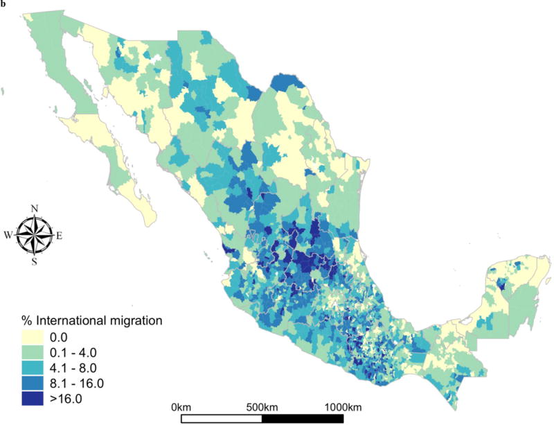
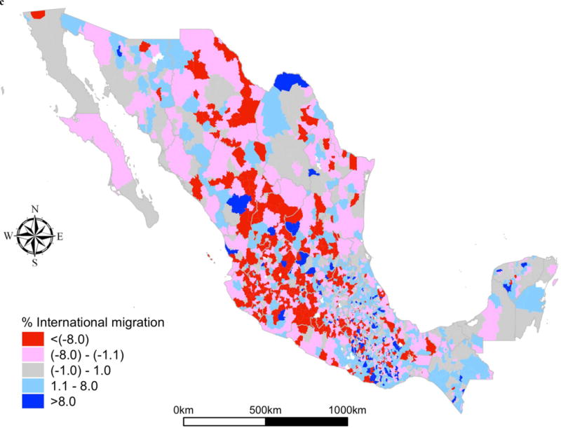
Undocumented Mexican migration peaked during the late 1990s and the early 2000s, and experienced a very sizable decline beginning around 2006 (Passel et al. 2012, Passel and Cohn 2016).The high point of Mexico – US migration (see Figure 1a) was likely due to a confluence of favorable labor demand in sectors of the US economy employing immigrants (Kandel and Parrado 2005), economic uncertainty in much of urban Mexico in the mid-late 1990s (Garip 2017), and poor conditions in the Mexican countryside after NAFTA (Nevins 2007); all of which were facilitated by large/dense active migrant networks (Massey and Riosmena 2010). As latent, root causes of the slowdown (see Figures 1b and 1c) scholars have identified demographic factors, such as increasingly smaller cohorts of Mexicans entering the labor force and the second-round effects of this slowdown on the economy (see Hanson and McIntosh 2010), and more stable economic prospects and/or network maturation in traditional sending areas (e.g.,Burkham 2014). Yet, even if the decline is related to these secular changes, it was also clearly accelerated by the poor job market conditions in the US following the real estate and financial market crash of 2007 (Villarreal 2014). As also examined by Villarreal (2014), the increasingly-increasing rise in US border and interior immigration enforcement over the last decade also had a nontrivial if more minor role.

FIGURE 1.

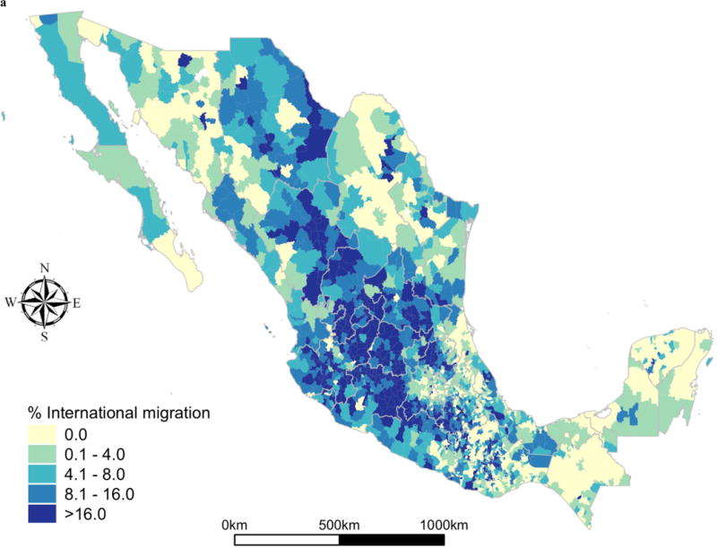
a Percent of households in municipality sending an international migrant in 1995‒1999

b Percent of households in municipality sending an international migrant in 2005‒2009

c Change in percent of households in municipality sending an international migrant in 2005‒2009 relative to 1995‒1999

As discussed in the vulnerability and adaptation literature (e.g., Eakin 2006), the association between climatic variability and migration is highly dependent on context. Thus, our use of the international outmigration modules included in the 2000 and 2010 Mexican Census long-form surveys –roughly covering the 1995–1999 and 2005–2009 periods– allows for the study continuity and changes in the climate-migration relationship during radically different contexts in Mexico and, especially, the United States. The comparison of two periods with such different migration conditions thus provides a unique opportunity to examine the extent to which somewhat different economic, social, and policy conditions may mediate environmental effects on migration.

Data and methods

The core data set employed for this analysis combines Mexican census data with high-resolution climate data, both obtained via the Terra Populus (TerraPop) extract system (Kugler 2015, MPC 2013, Nawrotzki et al. 2016b). The migration, demographic, and socioeconomic data available through TerraPop originate from the 2000 and 2010 Mexican census long form, collected by the Instituto Nacional de Estadística y Geografía (INEGI) and further harmonized by IPUMS International (MPC 2015a; Ruggles et al. 2003). We employed a 1.0% extract—a density commonly used in these types of analyses (e.g., Nawrotzki et al. 2013). On the assumption that environmental factors are more likely to affect residents in rural areas dependent on agriculture, ranching, or other climate-dependent activities (Mueller et al. 2014), we restricted our analysis to localities with fewer than 15,000 individuals. Most studies have used the official rural threshold of 2,500 inhabitants; we aim to include larger areas still heavily dependent on primary sector activities. Our selection yielded an analytic sample of 110,343 and 194,947 households for 2000 and 2010, respectively.

TerraPop allows linking various environmental data to census records up to its finest-resolution administrative level (the municipality in the public release of the census microdata). We use a gridded time series of high-resolution (0.5°, or 55km × 55km) monthly temperature (min, max) and precipitation readings generated by the Climate Research Unit (CRU) at the University of East Anglia (Harris et al. 2014). In addition, we linked a number of publicly available data sources to the core data set to obtain information on the municipality’s migration intensity, marginalization, irrigation type and crops planted, as well as state-level changes in GDP, described in detail below.

Outcome variable

The census long form included a section on international migration, in which respondents were asked whether any current or past member of the household had moved abroad during the five years before the interview. Though this measure clearly does not cover the emigration of whole households out of the country (see Hamilton and Savinar), Mexican migration has historically followed a sequential pattern in which one household member (often the household head) moves first for labor purposes and is followed by others after a few years (Cerrutti and Massey 2001, Hondagneu-Sotelo 1994). Further, this measure has the advantage of capturing not only the initial movement of specific members but also that of recurrent or “circular” migrants who returned to Mexico but emigrated again.³ While it is not possible to identify an individual’s country of destination in the IPUMS public release, the United States is by far the most common international destination of rural Mexicans.⁴ We therefore use the terms international and US-bound migration interchangeably.

Because migration decisions usually engage other family members (Cohen 2004, Hondagneu-Sotelo 1994, Taylor 1999), we study whether households sent at least one migrant abroad during the five years preceding the census round. Persons who left the country for vacation, temporary work assignments by their Mexico-based employers, visits to relatives, or other reasons that did not entail a change of residence were not considered migrants. As Table 1 shows, 5.3% of households had at least one member moving to an international destination between 2005 and the 2010 census date, centered on June 12. This is a sizable reduction from the 8.2% of households that sent a member to an international destination between 1995 and the 2000 census date in mid-February, reflecting the slowdown mentioned above (Passel and Cohn 2016, Passel et al. 2012). As Figure 1c shows, while decline occurred throughout most of the country, the most dramatic reductions occurred in traditional migrant-sending regions in the Central-West and Central-North along the western Sierra Madre (cf. Figure 1a).

Table 1.

Means and standard deviations of main analysis variables, by Census year

	Pooled		2000		2010
	Mean	(S.D.)	Mean	(S.D.)	Mean	(S.D.)
HH sent migrant abroad during 5 years prior to Census (%)	6.3	(24.4)	8.2	(27.4)	5.3	(22.4)
Maximum temperature, baseline (°C)	27.4	(3.1)	27.4	(3.2)	27.4	(3.1)
Temperature change during retrospective window (°C)	0.76	(0.27)	0.69	(0.31)	0.80	(0.24)
% months in window where temperature was... SDs above baseline
1 – 2 standard deviations	28.9	(7.9)	26.0	(8.3)	30.5	(7.1)
2+ standard deviations	7.8	(5.7)	8.1	(4.5)	7.6	(6.3)
Rainfall, baseline (mm/yr)	92.6	(49.0)	88.8	(47.2)	94.8	(49.8)
Precipitation change during retrospective window (mm/yr)	1.4	(51.6)	−1.7	(49.7)	3.1	(52.3)
% months in window where precipitation was… SDs below baseline
1 – 2 standard deviations	10.7	(7.0)	12.8	(6.3)	9.5	(7.2)
2+ standard deviations	0.5	(1.1)	0.7	(1.3)	0.4	(0.9)
Marginalization index (z-score)	0.15	(1.1)	−0.06	(1.0)	0.28	(1.1)
Economic diversity index (0–1)	0.67	(0.19)	0.66	(0.18)	0.67	(0.19)
International migration intensity index (z-score)	−0.02	(1.0)	0.05	(1.0)	−0.06	(1.0)
Municipal land classified as urban (%)	0.9	(4.06)	1.0	(4.05)	0.8	(4.07)
Municipal farmland that is irrigated (%)	18.3	(26.6)	20.6	(27.9)	17.0	(25.7)
Area of farmland planted with corn (sqm / 10 ha)	1.4	(1.5)	1.3	(1.4)	1.4	(1.5)
Area of farmland planted with wheat (sqm / 10 ha)	0.1	(0.26)	0.1	(0.27)	0.1	(0.25)
Area of farmland planted with soybeans (sqm / 10 ha)	0.1	(0.40)	0.1	(0.42)	0.0	(0.39)
2,500 – 14,999 inhab. in locality (REF = less than 2,500)	0.3	(0.47)	0.3	(0.46)	0.3	(0.47)
State GDP growth, window relative to prior 5 years (%)	3.08	(1.6)	2.10	(1.7)	3.64	(1.3)
HH members working in primary sector activities (%)	20.6	(27.4)	21.4	(28.1)	20.2	(27.0)
HH members employed (%)	33.3	(26.3)	32.6	(25.5)	33.6	(26.8)
Asset index (z-score)	0.0	(0.63)	−0.1	(0.63)	0.1	(0.61)
HH is owned by one of its members	0.9	(0.34)	0.8	(0.36)	0.9	(0.33)
Schooling of HH head (years)	4.8	(4.1)	4.5	(3.9)	5.0	(4.2)
HH income (in 1,000s MXN)	2.9	(10.0)	2.0	(12.3)	3.3	(8.5)
Age of HH head (years)	47.7	(17.0)	45.9	(16.6)	48.8	(17.1)
Children under 5 in HH (No.)	0.4	(0.67)	0.5	(0.73)	0.3	(0.63)
N (households)	305,290		110,343		194,947

Source: see Appendix I for specific variable sources.

Environmental exposure

Our analytical focus is the impact of climate variability on US migration. As Table 1 shows, the average maximum temperature in Mexico during 1960–1990— a period used in the climatological literature to represent “climate normal” conditions (Arguez and Vose 2011)—was 27.4 °C (81.3 °F). To further assess whether migration is related to warming, we estimated the difference between this climate normal and the temperature during the 6 years preceding the 2000 and 2010 census dates (hereafter, the “observation periods”) to allow for a lag between environmental shocks and migration (see Nawrotzki and DeWaard 2016). The average Mexican municipality experienced nontrivial warming relative to its climate normal, with maximum temperatures increasing 0.7 °C and 0.8 °C in the observation periods. As for precipitation, the average Mexican municipality received an average of 93 mm of rain per month during the climate normal period, experiencing a moderate average decline of 1.7 mm/month in 1994–2000 and a moderate average increase of 3.1 mm/month in 2004–2010.

Even when experiencing slightly above-average rainfall in 2004–2010, many Mexican municipalities experienced sizable declines in precipitation during some months within each observation period, with even larger shares of municipalities experiencing sizable temperature increases than rainfall declines. To assess both the frequency and the severity of this exposure, we used the monthly maximum temperatures to determine the percent of observation period months in which the average maximum temperature of a municipality surpassed the 30-year average maximum temperature by 1–1.99 and by 2 or more standard deviations (Nawrotzki and Bakhtsiyarava 2016). Henceforth, we refer to rainfall/temperature measures of 1 to 2 standard deviations below/above the climate normal mean as “severe” and those of 2+ standard deviations as “more severe.”

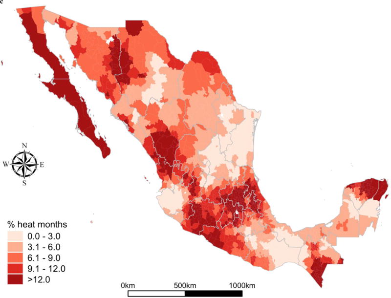
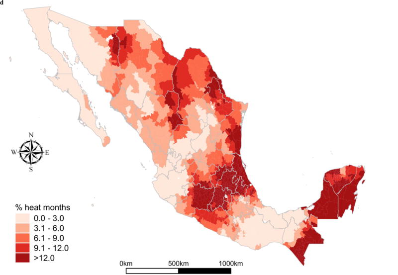
As Table 1 shows, Mexican municipalities experienced average maximum temperatures 1–1.99 standard deviations above their local climate-normal mean in 26% and 31% of the months in the observation period in 1994–2000 and 2004–2010, respectively. In addition to these nontrivial bouts of severe weather, municipalities experienced an additional 8.1% and 7.6% of months with average maximum temperatures at least 2 standard deviations above the climate normal, a substantial exposure to more serious climate extremes. The Northwest and Central parts of the country experienced some of the most extended episodes of severe and more severe heat in 2000 (see Figures 2a and 2c), while the North-Central, Central, and Eastern portions of the country experienced higher-frequency episodes (see Figures 2b and 2d).

FIGURE 2.

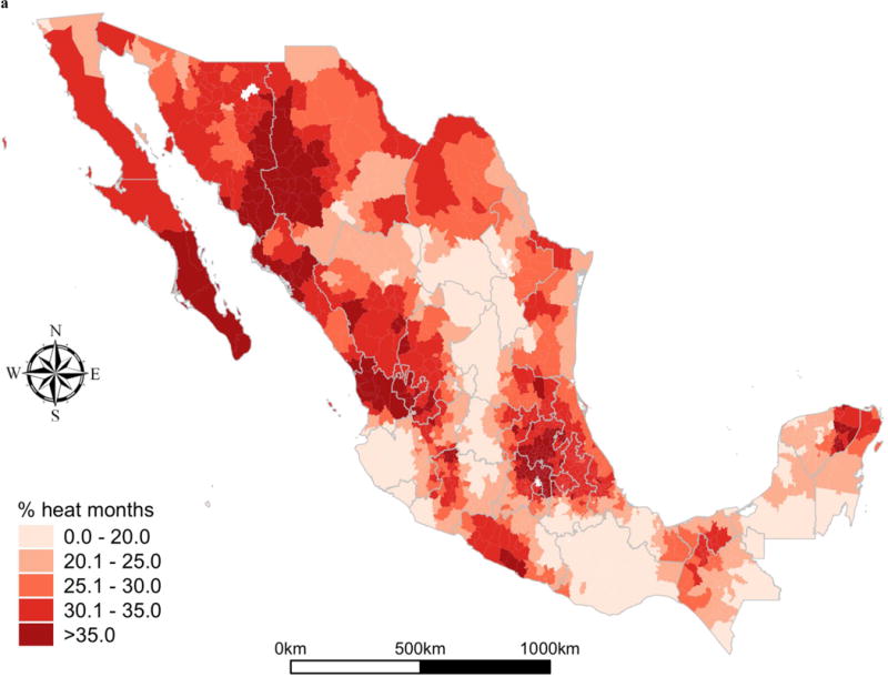
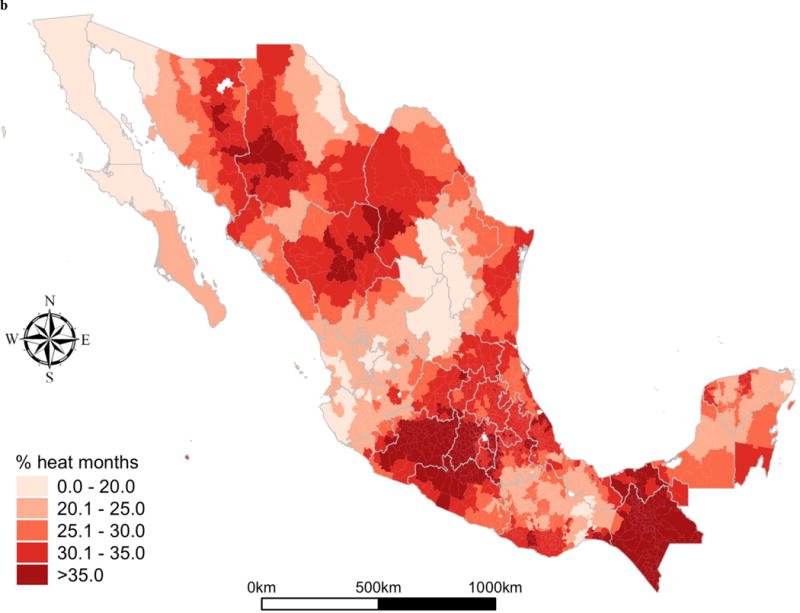
a Percent of months in municipality in 1995‒1999 when temperatures exceeded 1960‒1990 average by 1–1.99 standard deviations

b Percent of months in municipality in 2005‒2009 when temperatures exceeded 1960‒1990 average by 1–1.99 standard deviations

c Percent of months in municipality in 1995‒1999 when temperatures exceeded 1960‒1990 average by 2 or more standard deviations

d Percent of months in municipality in 2005‒2009 when temperatures exceeded 1960‒1990 average by 2 or more standard deviations

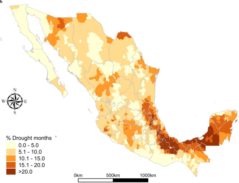
The Mexican territory experienced less prolonged periods of more severe drought. On average, precipitation was 1–1.99 standard deviations below the climate-normal average in roughly 13% and 10% of months in 1994–2000 and 2004–2010, respectively. As Figure 3a illustrates, most of the Northern border and most of the East experienced a higher frequency of severe droughts in 2000. In 2010, fewer municipalities experienced frequent severe droughts, and those that did were clustered along the southern portion of the Gulf of Mexico Coast, along with some in the Central-West and some in the northern border.

FIGURE 3.

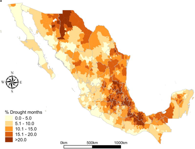
a Percent of months in municipality in 1995‒1999 when rainfall was below 1960‒1990 average by 1–1.99 standard deviations

b Percent of months in municipality in 2005‒2009 when rainfall was below 1960‒1990 average by 1–1.99 standard deviations

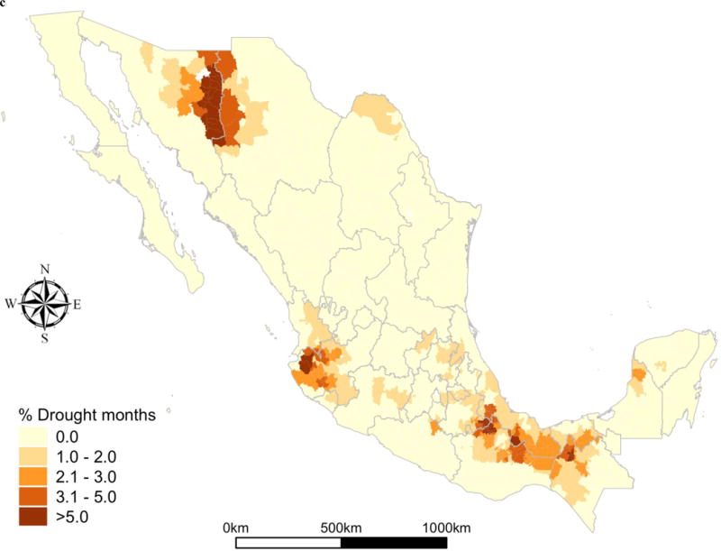
c Percent of months in municipality in 1995‒1999 when rainfall was below 1960‒1990 average by 2 or more standard deviations

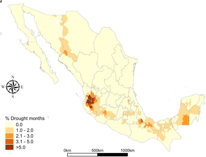
d Percent of months in municipality in 2005‒2009 when rainfall was below 1960‒1990 average by 2 or more standard deviations

Only 0.7% and 0.4% of months were characterized by rainfall 2 or more standard deviations below the long-term mean. In 2000, these “more severe” rainfall deficits were concentrated in clusters around the Sonora-Chihuahua border in the Northwest; Jalisco, Nayarit, and Colima in the Central-West; and the northern portions of Oaxaca and Chiapas along with Southern Tabasco and Southeastern Veracruz in the South (see Figure 3c). In 2010, the more severe drought occurred in the same Central-Western region, with less frequent episodes in the southern region described above (see Figure 3d).

Modulators of exposure: sensitivity and adaptive capacity

Table 1 also shows descriptive statistics of several sociodemographic characteristics that other studies of the environment-migration nexus and of Mexico-US migration suggest may mediate the climate-migration association. To account for the municipality’s social vulnerability (a combination of sensitivity and adaptive capacity), we employ a marginalization index developed by the Mexican National Population Council for 2000 and 2010 separately (see CONAPO 2011). This measure is a normalized index based on principal components analysis of nine different socioeconomic indicators derived from the census.⁵ Like any z-score metric, the index is designed to have a mean of 0 and a standard deviation of 1.

To further control for sensitivity, we also estimated the sector diversity of local labor markets. Rural places where employment is largely dependent on a few primary sector activities may be especially sensitive to climate because people lack alternative income and employment options. Thus, following Hamilton and Villarreal (2011), we calculated an index of employment in 18 different economic sectors. The index ranges from 0 (full concentration in one economic sector) to 1 (equal shares of employment in each of the 18 sectors), with a stable average of 0.66–0.67 across censuses. Even though we focus on the population living in small localities, these could be located near urban areas (Hamilton and Villarreal 2011) that may provide resources and alternative employment opportunities in sectors less sensitive to climatic variability. To proxy access to this urban infrastructure, we use the percentage of urban land in the municipality, using data on MODIS urban extent classifications available through TerraPop for 2000. Since, smaller, more rural locales in Mexico are increasingly located in remote areas, only 1% of these municipalities’ areas had considerable built-up (i.e., impervious surfaces).

Given that climate effects on migration dynamics operate largely through impacts on the agricultural sector (Feng and Oppenheimer 2012, Mastrorillo et al. 2016, Mueller et al. 2014, Nawrotzki et al. 2015a), we include a number of control variables aimed at capturing farming activities in each municipality. Because irrigation infrastructure is key to guarding against adverse drought effects (Gutmann and Field 2010), we used a measure of the percentage of farmland irrigated, computed from information on hectares of irrigated and rainfed planted surface available from the Mexican agricultural census for the years 2004–2009 (INEGI 2012a). Because there are no data available for a similar period in the 1990s, we assume time-invariance in the measure and used it for 1994–1999. On average, only roughly a fifth of the municipal farmland represented in our data was irrigated. Because crops vary in climate sensitivity, i.e., corn is less sensitive to temperature variability than soy, and to precipitation variability than either soy or wheat (see Lobell and Field 2007), we also included measures of the area planted with corn, wheat, and soybeans, the three primary crops in Mexico, constructed by the Global Landscape Initiative and available through IPUMS-TerraPop. Overall, the extent of corn production was at least 10 times greater than that of wheat and soy.

Finally, we include a measure of the extent of transnational migrant networks in sending areas. Established migrant networks count among the strongest factors influencing the probability of migration (Fussell and Massey 2004, Massey et al. 2010, Massey and Riosmena 2010). To measure these connections, we used the international migration intensity indices developed by CONAPO (2012), a composite standardized measure constructed in a similar fashion to the marginalization index above, in this case based on the percentage of households in the municipality sending or receiving at least one international migrant in the five years preceding the census (including circular migrants leaving and returning within the period), as well as the percentage of households receiving remittances from abroad.

Other controls

To avoid confounding the influence of climate variability with economic fluctuations in Mexico not caused by climate, we control for the change in state-level gross domestic product (GDP) during our observation window. Using data obtained from INEGI (2012a), we calculated the inflation-adjusted percentage growth in GDP for each year in reference to the preceding year, averaged across the 6-year period preceding the census round (i.e., 1994–1999–2004–2009).⁶

Finally, we control for the household’s life course stage and socioeconomic conditions. We use two measures of life-cycle stage to reflect differential human capital resources and needs across households (e.g., Riosmena 2009). Age of the household head is used as a general proxy for family life-cycle stage (VanWey et al. 2007). Nurturing activities may tie human capital to the household, and we reflect this by including a measure of its number of young children (age < 5 years). We further capture human capital by including the years of schooling of the household head. Studies often find lower levels of education among international migrants from Mexico, although this education selection is relatively weak (Rendall and Parker 2014).

We also include other measures of the household’s socioeconomic standing. One of the main motivations for sending a migrant abroad is to increase the household’s financial well-being by escaping liquidity constraints, often in response to both poor labor market opportunities and capital and insurance market failures (Stark and Bloom 1985). We attempt to capture this general motivation by including measures of household income and the percentage of adult household members employed. Because the income distribution was skewed, we log transformed this variable before using it in the multivariate models. To account for the dependence of a household’s financial wellbeing on climate-sensitive sectors (cf., Mueller et al. 2014), we included a measure that captures the percentage of household members employed in the primary sector (agriculture and forestry).

To control for the household’s physical capital, we use information on home ownership and dwelling characteristics. Using a procedure similar to that of (Mberu 2006), we measure dwelling quality (e.g., floor and roof material), possession of household amenities (e.g., refrigerator, TV, washer, cars), and access to services (e.g., sewage collection, type of water supply) with a normalized index based on 13 items (Cronbach’s alpha = 0.87).

Estimation strategy

Because migration is a social phenomenon that is influenced by factors operating at multiple scales, we employ hierarchical modeling. In addition to adjusting for clustering, our multilevel models also take into account differences in sample sizes at different levels and heteroscedastic error terms (Luke 2004). Multilevel models are particularly well suited for the study of population-environment interactions, in which aggregate-level effects (e.g., climate) are used to predict household-level outcomes (e.g., migration), and are frequently used in this field (e.g., Fussell et al. 2014, Hunter et al. 2013, Nawrotzki et al. 2013). We predict the odds of an international move for the i^th household in the j^th municipality located in the k^th state during census period t (m_ijkt) using the logit link function ${\sigma }_{\mathit{ijkt}}=lo{g}_e(\frac{m_{\mathit{ijkt}}}{1-m_{\mathit{ijkt}}})$

$${\sigma }_{\mathit{ijkt}}=b_0+b_1(\mathit{temp}{S}_{\mathit{jkt}})+b_2(\mathit{tempM}{S}_{\mathit{jkt}})+b_3(\mathit{precip}{S}_{\mathit{jkt}})+b_4(\mathit{precipM}{S}_{\mathit{jkt}})+{\displaystyle {\sum }_n^y{b}_n(x_z)+u_{\mathit{jk}}+v_k+w_t}$$ (1)

In equation 1, the parameter b₀ constitutes the conventional intercept and reflects the average probability of sending an international migrant to the United States. The effect of severe (S = 1–1.99 SD) and more severe (MS = 2+ SD) temperature and precipitation effects on international migration are captured by coefficients b₁ to b₄. All models control for the effect (b_n) of n to y sociodemographic and spatial characteristics (x_z), which may influence migration patterns at the household (ijk), the municipality (jk), or the state (k) level during each census period (t). The models include municipality (u_jk) random intercept terms and state-level fixed effects (v_k), which allow for the estimation of a different migration propensity for each unit within an aggregation level. While we generally pooled 2000 and 2010 census data and added period fixed effects (w_t), we tested for the extent of the climate-migration relationship and the role of modulators like marginalization and migration intensity in stratified models, discussed later.

Results

The effect of environmental stress on migration

Table 2 shows results from multilevel models applied to pooled 2000–2010 data, in which we gradually introduce controls for the social and economic vulnerability of places. All “effects” in the figure are presented as standardized coefficients, which allows for assessment of the general order of magnitude of climate variables as compared to socioeconomic indicators. In our base Model I, we include basic household-level controls as well as measures for the two temperature and two precipitation climate extremes (plus municipal random effects present in all models). In addition, we include two-way interactions between temperature and precipitation extremes of similar severity (i.e., 1–1.99 or 2+ standard deviations, centering these variables in all cases to facilitate interpretation of the interactions) to better characterize drought-like conditions, in which low rainfall is compounded by high temperatures through higher evapotranspiration rates (Diffenbaugh et al. 2015). Subsequent models include controls for different forms of sensitivity and adaptive capacity, in addition to state fixed effects. All models include census period fixed effects and municipal random effects.

Table 2.

Standardized regression coefficients predicting the likelihood that a household sends an international migrant in 5 year window prior to Census.

	I			II			III			IV			V			VI			VII			VIII
	βstd	(S.E.)	Sig.	βstd	(S.E.)	Sig.	βstd	(S.E.)	Sig.	βstd	(S.E.)	Sig.	βstd	(S.E.)	Sig.	βstd	(S.E.)	Sig.	βstd	(S.E.)	Sig.	βstd	(S.E.)	Sig.
Temp. 1–1.99 SDs above long-term mean	−0.038	(0.002)		−0.047	(0.002)		−0.093	(0.002)	†	0.065	(0.002)		−0.016	(0.002)		−0.022	(0.002)		−0.111	(0.002)	*	0.032	(0.002)
Precip. 1–1.99 SDs below long-term mean	−0.557	(0.002)	***	−0.594	(0.002)	***	−0.062	(0.002)		−0.496	(0.002)	***	−0.605	(0.002)	***	−0.621	(0.002)	***	−0.131	(0.002)	*	−0.199	(0.002)	***
Temp, × Precip 1 -1.99 SDs	−0.252	(0.000)	***	−0.261	(0.000)	***	−0.193	(0.000)	***	−0.320	(0.000)	***	−0.265	(0.000)	***	−0.274	(0.000)	***	−0.177	(0.000)	***	−0.210	(0.000)	***
Temp. 2+ SDs above long-term mean	−0.136	(0.003)	†	−0.104	(0.003)		−0.124	(0.003)	*	0.071	(0.003)		−0.122	(0.003)	†	−0.107	(0.003)		−0.098	(0.003)		−0.015	(0.003)
Precip. 2+ SDs below long-term mean	−0.355	(0.014)	***	−0.352	(0.013)	***	−0.256	(0.011)	***	−0.297	(0.013)	***	−0.344	(0.014)	***	−0.338	(0.013)	***	−0.252	(0.011)	***	−0.159	(0.012)	**
Temp, × Precip 2+ SDs	0.095	(0.003)	†	0.111	(0.003)	†	0.103	(0.002)	*	0.200	(0.003)	***	0.091	(0.003)		0.102	(0.003)	†	0.116	(0.002)	*	0.185	(0.002)	***
International migration intensity index (z-score)							3.023	(0.012)	***										2.966	(0.012)	***	2.653	(0.012)	***
Marginalization index (z-score)													0.498	(0.026)	***	0.259	(0.029)	*	0.490	(0.020)	***	0.194	(0.021)	*
Economic diversity index (0–1)													−0.038	(0.102)		0.052	(0.102)		−0.161	(0.087)	*	−0.241	(0.085)	***
State GDP growth, window relative to prior 5 years (%)													0.158	(0.007)	***	0.147	(0.007)	**	−0.041	(0.007)		0.052	(0.007)
Municipal farmland that is irrigated (%)				−0.215	(0.001)	*										−0.148	(0.001)		−0.120	(0.001)	†	0.048	(0.001)
Area of farmland planted with com (sqm /10 ha)				0.149	(0.018)											0.133	(0.018)		0.157	(0.012)	*	−0.105	(0.012)
Area of farmland planted with wheat (sqm /10 ha)				−0.098	(0.097)											−0.078	(0.097)		−0.005	(0.061)		−0.143	(0.070)	†
Area of farmland planted with soybeans (sqm /10 ha)				−0.131	(0.058)											−0.125	(0.058)		0.122	(0.036)	*	0.322	(0.035)	***
2,500 – 14,999 inhab. in locality (REF = less than 2,500)
Municipal land classified as urban (%)				−0.611	(0.006)	***										−0.560	(0.006)	***	−0.016	(0.004)		−0.196	(0.004)	**
HH members working in primary sector activities (%)				0.085	(0.000)	*										0.086	(0.000)	*	0.061	(0.000)		0.076	(0.000)	†
HH members employed (%)	−0.813	(0.000)	***	−0.837	(0.000)	***	−0.784	(0.000)	***	−0.804	(0.000)	***	−0.815	(0.000)	***	−0.838	(0.000)	***	−0.795	(0.000)	***	−0.800	(0.000)	***
Asset index (z-score)	2.011	(0.018)	***	2.277	(0.019)	***	1.709	(0.017)	***	1.990	(0.018)	***	2.057	(0.018)	***	2.288	(0.019)	***	2.046	(0.019)	***	2.066	(0.019)	***
HH is owned by one of its members	0.508	(0.026)	***	0.452	(0.026)	***	0.544	(0.026)	***	0.515	(0.026)	***	0.499	(0.026)	***	0.449	(0.026)	***	0.477	(0.026)	***	0.476	(0.026)	***
Schooling of HH head (years)	−1.278	(0.003)	***	−1.243	(0.003)	***	−1.195	(0.003)	***	−1.272	(0.003)	***	−1.277	(0.003)	***	−1.242	(0.003)	***	−1.157	(0.003)	***	−1.178	(0.003)	***
HH income (in 1,000s MXN)	−0.051	(0.001)		−0.025	(0.001)		−0.023	(0.001)		−0.054	(0.001)		−0.046	(0.001)		−0.024	(0.001)		−0.002	(0.001)		−0.003	(0.001)
Age of HH head (years)	−1.251	(0.001)	***	−1.242	(0.001)	***	−1.254	(0.001)	***	−1.262	(0.001)	***	−1.250	(0.001)	***	−1.242	(0.001)	***	−1.245	(0.001)	***	−1.268	(0.001)	***
Children under 5 in HH (No.)	−0.880	(0.015)	***	−0.888	(0.015)	***	−0.879	(0.015)	***	−0.888	(0.015)	***	−0.883	(0.015)	***	−0.889	(0.015)	***	−0.891	(0.015)	***	−0.889	(0.015)	***
2010 Census (REF = 2010 Census)	Yes			Yes			Yes			Yes			Yes			Yes			Yes			Yes
State fixed effects?	No			No			No			Yes			No			No			No			Yes
N (households)	305,290			305,290			305,290			305,290			305,290			305,290			305,290			305,290

^***p < 0.001

^**p < 0.01

^*p < 0.05

^†0.10

Source: pooled 2000 & 2010 Mexican Census long form sample data from IPUMS. see Appendix I for specific variable sources.

First, it is important to point out that the “effects” of our climate variables are considerably smaller than the implied effect of social and economic conditions in the household (e.g., asset index, schooling of the household head) and the municipality (most notably, the migration intensity index). However, the climate-migration associations in the analyses are far from being trivial. Regardless of the model examined, our estimates suggest that international migration is—on average—less likely during times of severe –but not the most severe– environmental stress. These “effects” are nontrivial: an increase of 1 standard deviation in the percentage of months with 1–1.99 standard deviations of below-normal precipitation is associated with half a standard deviation decrease in the probability of international migration. While extreme precipitation shortages are less common than extremes in higher temperatures (as Table 1 shows), their “effect” on migration is stronger in the sense that an increase of one standard deviation in the percent of months with 1–1.99 or 2+ standard deviations of precipitation below climate normal implies a larger decrease in migration than does a similar increase in above-normal temperatures. In addition, as illustrated in Figures 4a and 4b, note that severe heat and drought interact to suppress migration even more than would the sum of their separate effects (see Figures 4a and 4b).

FIGURE 4.

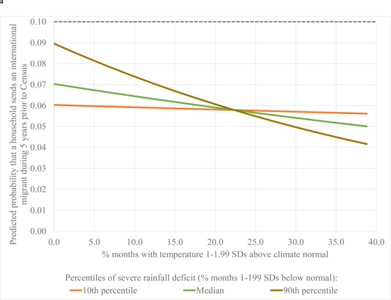
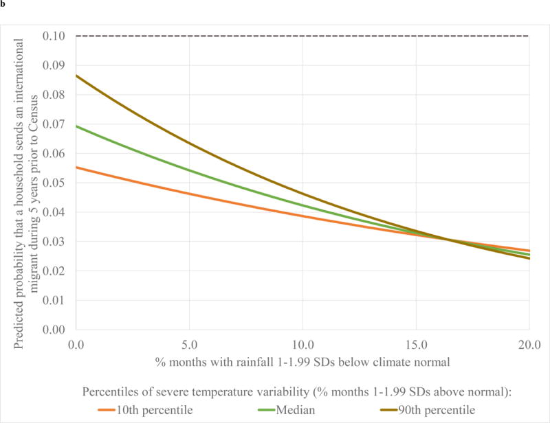
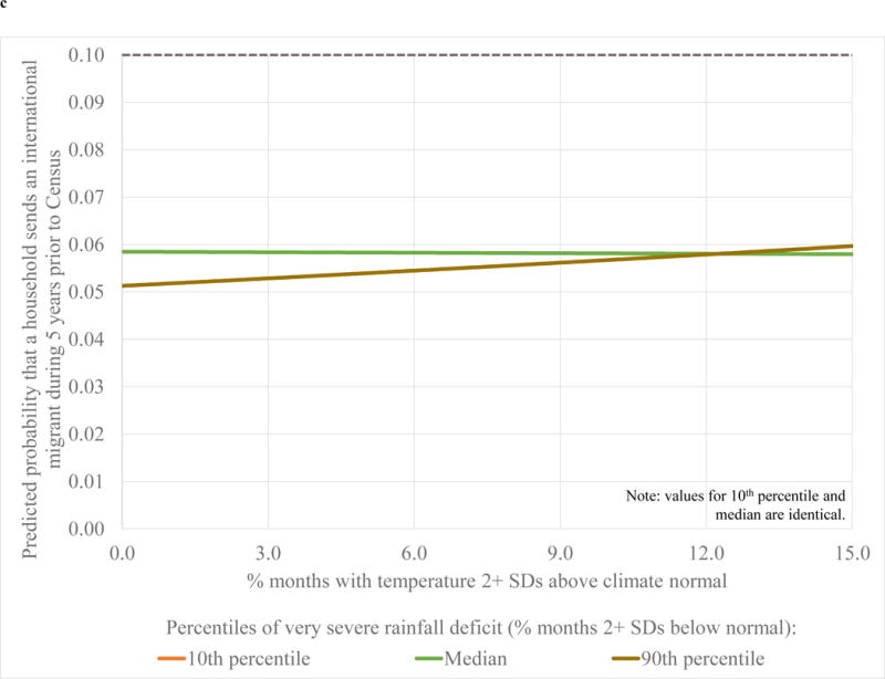
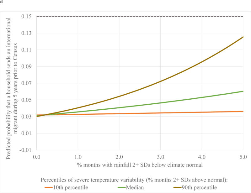
a Predicted probability that a rural Mexican household sends an international migrant according to the frequency of severe high temperatures for different levels of rainfall deficit severities.

b Predicted probability that a rural Mexican household sends an international migrant according to the frequency of severe rainfall deficits for different levels of high temperature severities.

c Predicted probability that a rural Mexican household sends an international migrant according to the frequency of very severe high temperatures for different levels of very severe rainfall deficits.

d Predicted probability that a rural Mexican household sends an international migrant according to the frequency of very severe rainfall deficits for different levels of very severe high temperatures.

Figures 4c and 4d show similar results for very severe high temperatures and rainfall deficits respectively. These results suggest that, while rural Mexicans were in general less likely to migrate to the United States during either the most severe relative increases in temperature or the most severe relative decreases in rainfall, they were indeed more prone to migrate in places experiencing very severe heat and drought conditions. As is evident in all models in Table 2, especially those controlling for socioeconomic conditions (III–VIII), a higher frequency of more severe temperature increases in places that also had more severe rainfall deficits implied a higher likelihood of migration (see Figure 4c). Likewise, more frequent episodes of more severe rainfall deficits were associated with higher US migration in places with above-median bouts of more severe temperature increases (see Figure 4d).

The modulating roles of sensitivity and adaptive capacity

Thus far, our results suggest that US migration is a particularly costly venture during times of environmental stress, but that extremely dire environmental conditions may motivate people to emigrate abroad (see also Nawrotzki et al. 2013). In addition, the environment-migration nexus—perhaps particularly in the case of costlier forms of (international, long-distance) movement—is likely to be contingent on social and economic contexts. To test this assertion more systematically than most prior studies had, Table 3 shows results from models presenting interactions between (A) climate extremes and the municipal marginalization index (models A.I– A.III), and (B) climate extremes and the municipal migration intensity index (models B.I–B.III). Models A.I and B.I show two-way interactions between each of our four climate extreme measures and marginalization and migration intensity, respectively. Models A.II and B.II are identical to A.I and B.I, except for the addition of two-way interactions between severe or more severe rainfall and precipitation frequency measures (as in all models presented in Table 2). Finally, Models A.III and B.III add three-way interactions between temperature, precipitation, and marginalization and migration intensity, respectively (in all models, all variables were centered at their mean to facilitate interpretation of their coefficients). In general, the addition of the two-way or three-way interactions did not change the climate-marginalization or climate-migration intensity relationships, so we discuss these in general terms.

Table 3.

Standardized regression coefficients predicting likelihood that a household sends an international migrant in 5 year window prior to Census.

	A. Climate ·Marginalization									B. Climate Migration intensity
	Pooled									Pooled
	A.I			A.II			A.III			B.I			B.II			Bill
	βstd	(S.E.)	Sig.	βstd	(S.E.)	Sig.	βstd	(S.E.)	Sig.	βstd	(S.E.)	Sig.	βstd	(S.E.)	Sig.	βstd	(S.E.)	Sig.
Temp. 1–1.99 SDs above mean	0.033	(0.002)		−0.018	(0.002)		−0.027	(0.002)		0.205	(0.002)	***	0.141	(0.002)	*	0.160	(0.002)	**
x marginalization index	0.257	(0.002)	***	0.243	(0.002)	***	0.202	(0.002)	***
x migration intensity index										−0.111	(0.001)	**	−0.103	(0.001)	*	−0.107	(0.001)	**
Precip. 1–1.99 SDs below mean	−0.044	(0.002)		−0.084	(0.002)		−0.086	(0.002)		−0.266	(0.002)	***	−0.289	(0.002)	***	−0.289	(0.002)	***
x marginalization index	−0.284	(0.002)	***	−0.281	(0.002)	***	−0.299	(0.002)	***
x migration intensity index										0.277	(0.002)	***	0.255	(0.002)	***	0.307	(0.002)	***
Temp, × Precip 1 – 1.99 SDs				−0.244	(0.000)	***	−0.233	(0.000)	***				−0.219	(0.000)	***	−0.308	(0.000)	***
Temp, × Precip 1 – 1.99 SDs × marginalizatior							−0.139	(0.000)	***
Temp, × Precip 1 – 1.99 SDs × migration intensity																0.214	(0.000)	***
Temp. 2+ SDs above mean	−0.009	(0.003)		0.023	(0.003)		0.028	(0.003)		−0.042	(0.003)		0.004	(0.003)		0.005	(0.003)
x marginalization index	−0.070	(0.003)		−0.053	(0.003)		−0.039	(0.003)
x migration intensity index										−0.018	(0.002)		−0.016	(0.002)		−0.003	(0.002)
Precip. 2+ SDs below mean	−0.172	(0.012)	***	−0.166	(0.012)	**	−0.184	(0.012)	***	−0.219	(0.013)	***	−0.217	(0.013)	***	−0.248	(0.013)	***
x marginalization index	−0.270	(0.012)	***	−0.299	(0.012)	***	−0.318	(0.013)	***
x migration intensity index										0.140	(0.009)	***	0.175	(0.009)	***	0.192	(0.009)	***
Temp, × Precip 2+ SDs				0.149	(0.002)	**	0.168	(0.002)	**				0.180	(0.002)	***	0.185	(0.002)	**
Temp, × Precip 2+ SDs × marginalization							0.022	(0.003)
Temp, × Precip 2+ SDs × migration intensity																	0.058	(0.002)
Migration intensity (z-score)	2.625	(0.012)	***	2.598	(0.012)	***	2.594	(0.012)	***	2.674	(0.013)	***	2.653	(0.013)	***	2.680	(0.013)	***
Marginalization index (z-score)	0.205	(0.021)	*	0.210	(0.021)	*	0.205	(0.021)	*	0.254	(0.021)	**	0.254	(0.021)	**	0.254	(0.021)	**
State fixed effects?	Yes			Yes			Yes			Yes			Yes			Yes
N (households)	305,290			305,290			305,290			305,290			305,290			305,290

^***p < 0.001

^**p < 0.01

^*p < 0.05

^†0.10

Source: pooled 2000 & 2010 Mexican Census long form sample data from IPUMS. see Appendix I for specific variable sources

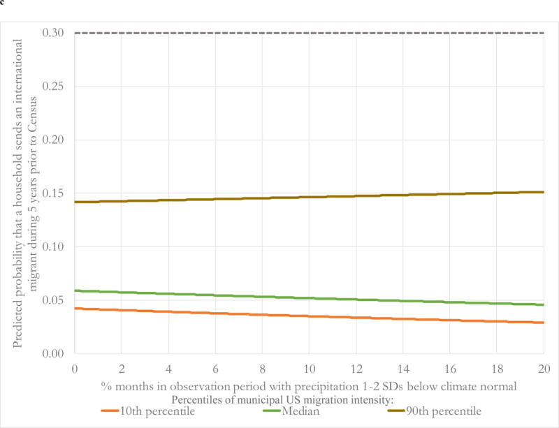
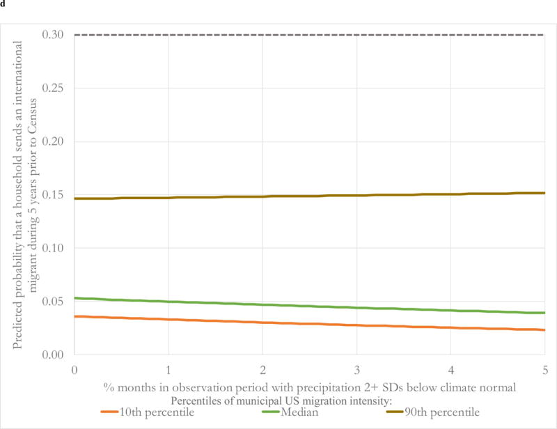
First of all, these results highlight that social and economic conditions do seem to modulate the relationship between climate stress and migration: except for the most severe (2+ SDs) temperature increases, all interactions between climate and marginalization, or between climate and migration intensity, are statistically significant. In the case of precipitation extremes (both severe and most severe), this means that US migration may be a response to poor rainfall among people living in areas with lower local sensitivity or higher adaptive capacity. This is illustrated in Figures 5a–5d (all derived from Model A.III in Table 3), where we present results of models with interactions between marginalization levels and (a) severe and (b) most severe rainfall declines as well as interactions between recent local migration intensity levels and (c) severe and (d) most severe rainfall deficits. All these figures show that drought-like conditions increase migration only in the least marginalized places (around the 10^th percentile of the municipal marginalization distribution), or in municipalities with the strongest transnational migrant networks (around the 90^th percentile of the migration intensity distribution). Virtually everywhere else, severe and most severe rainfall deficits are associated with lower US-bound migration, as indicated by the other two lines in each graph, representing the median and 90^th (10^th) percentile of the marginalization (migration intensity) distribution.

FIGURE 5.

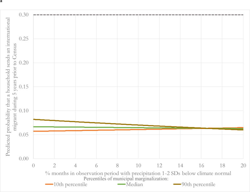
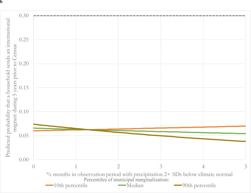
a Predicted probability that a rural Mexican household sends an international migrant according to the frequency of severe precipitation deficits (1‒2 SDs below normal) for different levels of municipal marginalization.

b Predicted probability that a rural Mexican household sends an international migrant according to the frequency of very severe precipitation deficits (2+ SDs below normal) for different levels of municipal marginalization.

c Predicted probability that a rural Mexican household sends an international migrant according to the frequency of severe precipitation deficits (1‒2 SDs below normal) for different levels of municipal US migration intensity.

d Predicted probability that a rural Mexican household sends an international migrant according to the frequency of very severe precipitation deficits (2+ SDs below normal) for different levels of municipal US migration intensity.

In sharp contrast, a higher frequency of severe heat is associated with (slightly) higher US migration only in places with higher sensitivity or lower adaptive capacity. Figures 6a and 6b show that a higher percentage of months with severe increases in temperature is associated with higher migration in the most marginalized municipalities (those around the 90^th percentile; see Figure 6a) or in those with the lowest recent migration intensity (those in the 10^th percentile; see Figure 6b). Indeed, as both figures also show, in municipalities with lower marginalization or higher recent migration intensity, this relationship is (mildly) negative. Finally, note that, while we observed a similar pattern for the frequency of most severe temperature increases, the interactions between these measures of climatic stress and marginalization/migration intensity were not statistically significant. Thus, we chose to not depict them graphically.

FIGURE 6.

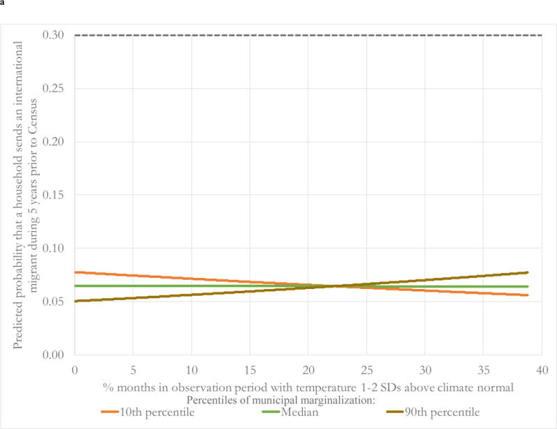
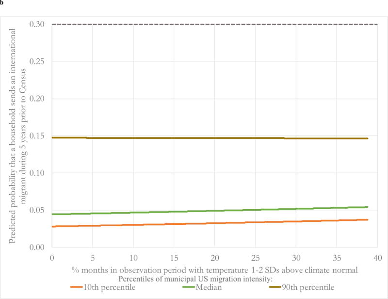
a Predicted probability that a rural Mexican household sends an international migrant according to the frequency of temperature increases (1‒2 SDs above normal) for different levels of municipal marginalization.

b Predicted probability that a rural Mexican household sends an international migrant according to the frequency of temperature increases (1–2 SDs above normal) for different levels of municipal US migration intensity.

The climate-migration nexus at the peak and slowdown of the Great Mexican Emigration Era

Finally, to assess whether the environment-migration nexus differed at the peak of the Great Emigration Era vs. the more recent significant (and persistent) slowdown, we examined the relationships described in Tables 2 and 3 according to census period (see Appendix II for a summary of results). With few exceptions, these analyses show that the association between climatic variability and migration was quite similar or otherwise stronger in 2005–2009 relative to these same relationships in 1995–1999.

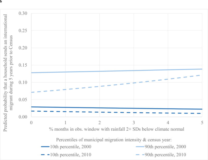
To illustrate, Figures 7a and 7b show results for very severe rainfall deficits across the extremes of the marginalization and migration intensity distributions, respectively. In both cases, the slope of the relationships in each municipality type (e.g., low marginalization or high migration intensity) are very similar in 2000 and 2010. One one hand, this suggests that the very different (destination) conditions between the two periods, likely not controlled for in the models via the year fixed effect, did not seem to disproportionately affect climate-induced migration. However, because migration did decrease considerably in 2005–2009 relative to 1995–1999, it is likely that the dramatic slowdown in (undocumented) US-bound migration from Mexico reduced the number of likely “environmental migrants” even if it did not substantially alter the relationship between climate and migration.

FIGURE 7.

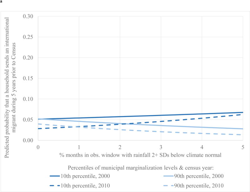
a Predicted probability that a rural Mexican household sends an international migrant according to the frequency of very severe rainfall deficits (2+ SDs below normal) for different levels of municipal marginalization, by census year.

b Predicted probability that a rural Mexican household sends an international migrant according to the frequency of very severe rainfall deficits (2+ SDs below normal) for different levels of municipal US migration intensity, by census year.

Conclusions

Our study contributes to the understanding of the relationship between climate change/variability, international population mobility, and development in several ways. First, using data representing a broader set of contexts of emigration and conditions in the United States than examined in prior work, we show that the climate-US migration nexus in rural Mexico is highly situated/variable, with a negative association between climate shocks and migration in (most) places and a positive one in (a few) others. Consistent with findings across the developing world, which suggest that climate migration is more likely to be internal and shorter-distance (e.g Henry et al. 2004, Massey et al. 2010) or to otherwise “trap” populations under specific conditions (Gray 2009, Gray 2010, Gray and Mueller 2011), we find that a higher frequency of severe climate conditions is associated with lower international migration rates across the vast majority of Mexican rural or primary sector-dependent communities. We stop short of arguing that our findings are clear indication of a trapping mechanism, however, as our study did not examine whether U.S. migration is substituted for lower-risk forms of population mobility within Mexico during times of climatic variability.

Despite this average negative association, which held for most municipalities across the socioeconomic and migration intensity continuum, consistent with prior work on Mexico – U.S. migration (Munshi 2003, Nawrotzki et al. 2013, Feng and Oppenheimer 2012, Jessoe et al. 2016) we did find positive associations between climate shocks and migration in specific climate or social conditions that line up with each of the three dimensions of vulnerability used in the climate literature (e.g., Adger 2006), namely exposure (strength of climate signal), sensitivity (actual impact of signal), and adaptive capacity (ability to cope with impact of signal). First, international movement is more likely with particularly pronounced environmental exposure, that is very severe increases in temperatures taking place in tandem with very severe decreases in rainfall (Figures 4a–4d; also see Nawrotzki et al. 2013). Given the generally-negative relation between climate and migration and the particularly dire level of environmental exposure at which the association is positive, this finding likely reflects a type of mobility people may only resort to in desperate situations and despite the high costs of migration. On the other hand, second, we also find that US migration is a response to severe or very severe rainfall (but not temperature) declines in places with low marginalization levels (Figures 5a–5b, and 6a), presumably because rural or primary sector dependent places with low marginalization are less sensitive to environmental exposures, thus allowing families to afford using migration in response to climate-related shocks. Alternatively, families living in communities with low marginalization levels may have a higher capacity to cope with or adapt to the negative impacts of environmental exposure, indeed using US migration as one coping strategy. Third, people from municipalities with very high migration intensities are more likely to migrate to the US during times of severe precipitation deficits (see Figures 5c–5d and 6b). This relationship may be expressing the well-known notion that stronger migrant networks reduce the costs and risks associated with mobility, thus loosening budget constraints that prevent people from moving internationally to cope or adapt to the impacts of (climate) shocks and in which the ability to migrate is a form of (extra-local) adaptive capacity.

Our results showing a positive association between climate and US migration in places with the highest municipal migration intensity are inconsistent with prior work with MMP data by Nawrotzki et al. (2015b), who find lower likelihoods of climate-related US migration from localities with a higher proportion of prior U.S. migrants. Nawrotzki et al.’s finding could be explained by the fact that translocal connections created by migration –and remittances sent from abroad in particular– are reducing households’ and communities’ vulnerability to climate change by either lowering local sensitivity to environmental exposure (e.g., via investment in irrigation systems, drought-resistant crops, and other impact mitigation strategies); or by improving their adaptive capacity via mechanisms other than the additional migration of fellow community members (e.g., by diversifying economic opportunities in sending areas). Because we use a broader sample across a larger variety of rural social contexts, we argue that the amplification mechanism we found likely dominates the more localized relationships found by Nawrotzki and colleagues’ with a more specialized sample (nevertheless, with good local representation). Future research should attempt to understand and reconcile these possible mechanisms while also examining whether these discrepancies could be explained by differences in the spatial scale or the operational definition of migrant networks used in the two studies.

In addition to contributing to the understanding of the relationships between population, development, and the environment by uncovering systematic variation in the climate-migration association e.g., across the rural development and migration intensity spectra, our findings on the heterogeneity of climate impacts on US migration also call for more caution in the elaboration of international “climate refugee” projections, certainly out of Mexico but likely of other nations as well. While work on climate migrant projections does implicitly consider the role of socioeconomic conditions in sending areas in “producing” differing amounts of migrants, this is because places are assumed to vary only in compositional, but not necessarily in structural terms. A more dynamic model, allowing for negative and positive effects of climate on migration (e.g., across social vulnerability continua), and allowing for a dynamic, stochastic evolution of migrant networks (see Massey and Zenteno 1999, De Haas 2010) would add a more appropriate level of complexity and uncertainty around the future climate refugee question.

Indeed, our study’s findings suggest that climate migrant projections out of rural Mexico are unlikely to be nowhere as high as those estimated by Feng and colleagues (2010, see also Feng and Oppenheimer 2012), who put climate migration from rural Mexico to the US in 2005–2080 at 1.4–6.7 million additional people (i.e., 2%–10% of the rural population of the country) across different adaptation scenarios. Instead, our findings suggest much smaller net figures – considering both the decline in migration in most places and the increase in migration in less marginalized, more migration-intense areas. These estimates may be perhaps more in line with the numbers of climate migrants forecasted by Jessoe et al. (2016), who estimate that 0.05%– 0.25% of the Mexican rural population will migrate to the U.S. for climate-related reasons by 2075.

Social and economic development policies designed to avoid more severe forms of displacement, as well as more direct expressions of vulnerability to climate and other shocks, would benefit from further distinguishing which kinds rural places may be more likely to lose population (internationally as well as internally) due to climate change, and in which ones may climate change actually depress mobility, potentially “trapping” populations in place and causing further dislocations and hindering their wellbeing, or otherwise altering internal mobility patterns. Indeed, policy recommendations in the population and climate change literature generally of course include any and all actions aimed at reducing vulnerability to climate by reducing exposure or sensitivity, or by improving adaptive capacity (e.g., MacKellar et al. 1998). However, because climate migration can be a last-resort option to the negative effects of climate (McLeman and Smit 2006) or as a form of extralocal adaptive capacity (Eakin 2005), these policies may reduce some forms of migration while potentially increasingly allow for others. Indeed, the goal of social policy (at least from the sending area perspective) should not be to reduce migration per se, but to reduce the likelihood of resorting to it in desperation, out of persecution or by more or less direct displacement, and that it does operate in a humane fashion.

Finally, while our study design did not allow us to explicitly control for specific economic and immigration policy conditions in destinations, our examination of two periods with radically different “contexts of reception” in the United States (in terms of labor demand and, to a lesser extent, immigration enforcement) does offer some insights on the possible role of destination-area conditions in climate and other forms of migration. On the one hand, the climate migration association was similar, or (in some cases) even stronger in 2005–2009 than in 1995–1999 (see Figures 7a–7b). However, as also clearly depicted in Figures 7a and 7b, (environmental and other) migration levels in 2005–2009 were somewhat lower than those observed in 1995–1999. Thus, our study suggests that climate migration is just as or, perhaps, just slightly less sensitive to these destination based conditions relative to other forms of international movement, meaning it may be somewhat sensitive to economic and, to a lesser extent, policy conditions (see Villarreal 2014). Future research on the environmental drivers of migration, as well as that devoted to design climate projections, should address the potential role destination contexts on the level of climate-induced migration.

Clearly, the climate-international migration relationship is complex and highly situated. As such, scholarship and policymaking on issues surrounding climate change need to continue moving away from simple conceptions that exposure to dire environmental conditions may be accompanied by a rising migrant tide, just as more purely “economic” types of migration are also quite heterogeneous (Garip 2012, Garip 2017, Riosmena 2009). Instead, research, scholarship, and policy should be designed with the idea that increasing environmental exposure can lead to divergent outcomes depending on how institutions, networks, and other social structures mediate the sensitivity of a place to a changing climate, and that these structures need not be –and are oftentimes not– local.

Appendix I.

Data sources for variables used in the analysis

Variable	Source
HH sent migrant abroad during 5 years prior to Census (%)	IPUMS
Maximum temperature, baseline (°C)	TerraPop
Temperature change during retrospective window (°C)	TerraPop
% months in window where temperature was... SDs above	TerraPop
1 – 2 standard deviations	TerraPop
2+ standard deviations	TerraPop
Rainfall, baseline (mm/yr)	TerraPop
Precipitation change during retrospective window (mm/yr)	TerraPop
% months in window where precipitation was… SDs below	TerraPop
1 – 2 standard deviations	TerraPop
2+ standard deviations	TerraPop
International migration intensity index (z-score)	CONAPO
Marginalization index (z-score)	CONAPO
Economic diversity index (0–1)	Population Census (100% data)
State GDP growth, window relative to prior 5 years (%)	Economic Census
Municipal farmland that is irrigated (%)	Agricultural Census
Area of farmland planted with corn (sqm / 10 ha)	Agricultural Census
Area of farmland planted with wheat (sqm / 10 ha)	Agricultural Census
Area of farmland planted with soybeans (sqm / 10 ha)	Agricultural Census
2,500 – 14,999 inhab. in locality (REF = less than 2,500)	IPUMS
Municipal land classified as urban (%)	IPUMS
HH members working in primary sector activities (%)	IPUMS
HH members employed (%)	IPUMS
Asset index (z-score)	IPUMS
HH is owned by one of its members	IPUMS
Schooling of HH head (years)	IPUMS
HH income (in 1,000s MXN)	IPUMS
Age of HH head (years)	IPUMS
Children under 5 in HH (No.)	IPUMS

IPUMS = 2000 & 2010 Mexican Population and Housing Census Long Form, 1% extract TerraPop: INSERT YEAR-YEAR Weather station data from the University of East Anglia’s CONAPO: Mexican National Population Council intensity indices calculated upon 2000 & 201 INEGI – Economic Census

Appendix II.

Regression coefficients predicting likelihood that a household sends an international migrant in 5 year window prior to Censu

	A. Model with interactions between climate variables, and census year
	Deviations 1–1.99 SDs above/below normal						Deviations 2+ SDs above/below normal
	Temperature increase			Rainfall deficits			Temperature increase			Rainfall deficits
	b	(S.E.)	sig.	b	(S.E.)	sig.	b	(S.E.)	sig.	b	(S.E.)	sig.
Climate var. main effect	−0.0025	(0.0022)		−0.0139	(0.0030)	***	0.0084	(0.0046)	†	−0.0342	(0.0141)	*
2-way interactions both climate vars.	−0.0011	(0.0003)	***	−0.0011	(0.0003)	***	0.0018	(0.0027)		0.0018	(0.0027)
2-way interact, climate var. & year	0.0070	(0.0038)	†	0.0104	(0.0034)	* *	−0.0107	(0.0051)	*	0.0573	(0.0233)	*
3-way interact, both climate vars. & year	−0.0004	(0.0005)		−0.0004	(0.0005)		0.0199	(0.0044)	***	0.0199	(0.0044)	***
	B. Model with interactions between climate variables, census year, and marginalization index
	b	(S.E.)	sig.	b	(S.E.)	sig.	b	(S.E.)	sig.	b	(S.E.)	sig.
Climate var. main effect	−0.0023	(0.0023)		−0.0130	(0.0030)	***	0.0096	(0.0047)	*	−0.0422	(0.0154)	**
2-way interactions both climate vars.	−0.0015	(0.0003)		−0.0015	(0.0003)	***	−0.0016	(0.0031)		−0.0016	(0.0031)
2-way interact, climate var. & year	0.0045	(0.0039)		0.0163	(0.0035)	***	−0.0076	(0.0054)		0.0649	(0.0256)	*
2-way interact, climate & margin.	0.0071	(0.0023)	**	−0.0120	(0.0031)	***	0.0097	(0.0049)	*	−0.0585	(0.0156)	***
3-way interact, both climate vars. & year	0.0003	(0.0005)		0.0003	(0.0005)		0.0286	(0.0048)	***	0.0286	(0.0048)	***
3-way interact, climate, year, & margin.	−0.0074	(0.0040)	†	0.0041	(0.0039)		−0.0144	(0.0058)	*	−0.0943	(0.0283)	***
-way int. bet. climate variables & margin.	−0.0003	(0.0006)		−0.0003	(0.0006)		−0.0048	(0.0055)		−0.0048	(0.0055)
	C. Model with interactions between climate variables, census year, and migration intensity index
	b	(S.E.)	sig.	b	(S.E.)	sig.	b	(S.E.)	sig.	b	(S.E.)	sig.
Climate var. main effect	0.0024	(0.0026)		−0.0174	(0.0032)	***	0.0031	(0.0052)		−0.0506	(0.0159)	**
2-way interactions both climate vars.	−0.0014	(0.0003)		−0.0014	(0.0003)	***	0.0023	(0.0033)		0.0023	(0.0033)
2-way interact, climate var. & year	0.0051	(0.0041)		0.0132	(0.0036)	***	−0.0020	(0.0057)		0.0265	(0.0267)
2-way interact, climate & mig. intensity	−0.0030	(0.0017)	†	0.0183	(0.0025)	***	0.0139	(0.0037)	***	0.0408	(0.0108)	***
3-way interact, both climate vars. & year	−0.0004	(0.0005)		−0.0004	(0.0005)		0.0168	(0.0050)	***	0.0168	(0.0050)	***
way interact, climate, year, & mig. intens.	−0.0036	(0.0033)		−0.0132	(0.0032)	***	−0.0097	(0.0048)	*	0.0677	(0.0257)	**
y int. bet. climate variables & mig. intens.	−0.0015	(0.0005)	**	−0.0015	(0.0005)	**	0.0114	(0.0049)	*	0.0114	(0.0049)	*

^***p < 0.001

^**p < 0.01

^*p < 0.05

^†0.10

^ΦΦΦModel includes all additional controls included in Model B.III, Table 3.

References

- Adger WN. Vulnerability. Global Environmental Change. 2006;16(3):268–281. [Google Scholar]
- Arguez A, Vose RS. The definition of the standard WMO climate normal: The key to deriving alternative climate normals. Bulletin of the American Meteorological Society. 2011;92(6):699–704. [Google Scholar]
- Bardsley D, Hugo G. Migration and climate change: examining thresholds of change to guide effective adaptation decision-making. Population & Environment. 2010;32(2):238–262. [Google Scholar]
- Barrios Puente G, Perez F, Gitter RJ. The Effect of Rainfall on Migration from Mexico to the US. International Migration Review 2015 [Google Scholar]
- Bindoff NL, Stott PA, Achutarao KM, Allen MR, Gillett N, Gutzler D, Hansingo K, Hegerl G, Hu Y, Jain S, Mokhov II, Overland J, Perlwitz J, Sebbari R, Zhang X. “Detection and Attribution of Climate Change: From Global to Regional.” in Climate Change 2013: The Physical Science Basis. Contribution of Working Group 1 to the Fifth Assessment Report of the Intergovernmental Panel on Climate Change. In: STOCKER TF, Q D, PLATTNER GK, TIGNOR M, ALLEN SK, BOSCHUNG J, NAUELS A, XIA Y, BEX V, MIDGLEY PM, editors. Climate Change 2013: The Physical Science Basis Contribution of Working Group I to the Fifth Assessment Report of the Intergovernmental Panel on Climate Change. New York: Cambridge University Press; 2013. [Google Scholar]
- Black R, Adger WN, Arnell NW, Dercon S, Geddes A, Thomas D. The effect of environmental change on human migration. Global Environmental Change. 2011;21:S3–S11. [Google Scholar]
- Bohra-Mishra P, Oppenheimer M, Hsiang SM. Nonlinear permanent migration response to climatic variations but minimal response to disasters. Proceedings of the National Academy of Sciences. 2014;111(27):9780–9785. doi: 10.1073/pnas.1317166111. [DOI] [PMC free article] [PubMed] [Google Scholar]
- Burkham JM. The End of Migration from Atotonilco El Bajo to Milwaukee: Breakdown of a Transnational Labor Market. Journal of Latin American Geography. 2014;13(3):113–136. [Google Scholar]
- Caney S. Climate change, human rights, and moral thresholds. In: GARDINER SM, C S, JAMIESON D, SHUE H, editors. Climate Ethics: Essential Readings. New York: Oxford University Press; 2010. [Google Scholar]
- Cattaneo C, Peri G. The migration response to increasing temperatures. Journal of Development Economics 2016 [Google Scholar]
- Cerrutti M, Massey DS. On the Auspices of Female Migration From Mexico to the United States. Demography. 2001;38(2):187–200. doi: 10.1353/dem.2001.0013. [DOI] [PubMed] [Google Scholar]
- Cohen JH. The culture of migration in Southern Mexico. Austin: University of Texas Press; 2004. [Google Scholar]
- Conapo. Índices de Marginación 2010 por Entidad Federativa y Municipio. Mexico City: Consejo Nacional de Población; 2011. http://www.conapo.gob.mx/es/CONAPO/Indices_de_Marginacion_2010_por_entidad_federativa_y_municipio. Last accessed October 5, 2016. [Google Scholar]
- Conapo. Índices de intensidad migratoria México-Estados Unidos. Mexico City: Consejo Nacional de Población; 2012. http://www.conapo.gob.mx/swb/CONAPO/Indices_de_intensidad_migratoria_Mexico-Estados_Unidos_2010. Last accessed October 5, 2016. [Google Scholar]
- De Haas H. The internal dynamics of migration processes: A theoretical inquiry. Journal of ethnic and migration studies. 2010;36(10):1587–1617. [Google Scholar]
- De Janvry A, Sadoulet E, De Anda GG. NAFTA and Mexico’s maize producers. World Development. 1995;23(8):1349–1362. [Google Scholar]
- De Sherbinin A, Warner K, Ehrhart C. Casualties of climate change. Scientific American. 2011;304(1):64–71. doi: 10.1038/scientificamerican0111-64. [DOI] [PubMed] [Google Scholar]
- Diffenbaugh NS, Swain DL, Touma D. Anthropogenic warming has increased drought risk in California. Proceedings of the National Academy of Sciences. 2015;112(13):3931–3936. doi: 10.1073/pnas.1422385112. [DOI] [PMC free article] [PubMed] [Google Scholar]
- Dillon A, Mueller V, Salau S. Migratory responses to agricultural risk in northern Nigeria. American Journal of Agricultural Economics. 2011;93(4):1048–1061. [Google Scholar]
- Durand J, Massey DS. Clandestinos: Migración México-Estados Unidos en los Albores del Siglo XXI. Zacatecas: Universidad Autónoma de Zacatecas; 2003. [Google Scholar]
- Durand J, Massey DS, Zenteno RM. Mexican immigration to the United States: Continuities and changes. Latin American Research Review. 2001;36(1):107–127. [PubMed] [Google Scholar]
- Eakin H. Institutional change, climate risk, and rural vulnerability: Cases from Central Mexico. World Development. 2005;33(11):1923–1938. [Google Scholar]
- Eakin H, Winkels A, Sendzimir J. Nested vulnerability: exploring cross-scale linkages and vulnerability teleconnections in Mexican and Vietnamese coffee systems. Environmental Science & Policy. 2009;12(4):398–412. [Google Scholar]
- Eakin HC. Weathering risk in rural Mexico: climatic, institutional, and economic change. Tucson: University of Arizona Press; 2006. [Google Scholar]
- Feng S, Krueger AB, Oppenheimer M. Linkages among climate change, crop yields and Mexico–US cross-border migration. Proceedings of the National Academy of Sciences. 2010;107(32):14257–14262. doi: 10.1073/pnas.1002632107. [DOI] [PMC free article] [PubMed] [Google Scholar]
- Feng S, Oppenheimer M. Applying statistical models to the climate–migration relationship. Proceedings of the National Academy of Sciences. 2012;109(43):E2915–E2915. doi: 10.1073/pnas.1212226109. [DOI] [PMC free article] [PubMed] [Google Scholar]
- Findley SE. Does Drought Increase Migration? A Study of Migration from Rural Mali during the 1983–1985 Drought. International Migration Review. 1994;28(3):539–553. [PubMed] [Google Scholar]
- OFFICE, U. G. S. F., editor. Foresight. Migration and Global Environmental Change. London, United Kingdom: 2011. [Google Scholar]
- Fussell E, Hunter LM, Gray CL. Measuring the environmental dimensions of human migration: The demographer’s toolkit. Global Environmental Change. 2014:28182–191. doi: 10.1016/j.gloenvcha.2014.07.001. [DOI] [PMC free article] [PubMed] [Google Scholar]
- Fussell E, Massey DS. The limits to cumulative causation: International migration from Mexican Urban Areas. Demography. 2004;41(1):151–171. doi: 10.1353/dem.2004.0003. [DOI] [PubMed] [Google Scholar]
- Garip F. Discovering diverse mechanisms of migration: The Mexico–US Stream 1970–2000. Population and Development Review. 2012;38(3):393–433. [Google Scholar]
- Garip F. On the Move: Changing Mechanisms of Mexico-US Migration. Princeton: Princeton University Press; 2017. [Google Scholar]
- Gemenne F. Why the numbers don’t add up: A review of estimates and predictions of people displaced by environmental changes. Global Environmental Change. 2011;21:S41–S49. [Google Scholar]
- Giné X, Townsend R, Vickery J. Patterns of rainfall insurance participation in rural India. The World Bank Economic Review. 2008;22(3):539–566. [Google Scholar]
- Goldman MJ, Riosmena F. Adaptive capacity in Tanzanian Maasailand: Changing strategies to cope with drought in fragmented landscapes. Global Environmental Change. 2013;23(3):588–597. doi: 10.1016/j.gloenvcha.2013.02.010. [DOI] [PMC free article] [PubMed] [Google Scholar]
- González De La Rocha M. From the Resources of Poverty to the Poverty of Resources? The Erosion of a Survival Model. Latin American Perspectives. 2001;28(4):72–100. [Google Scholar]
- Gray C. Environment, Land, and Rural Out-migration in the Southern Ecuadorian Andes. World Development. 2009;37(2):457–468. [Google Scholar]
- Gray C, Mueller V. Drought and population mobility in rural Ethiopia. World Development. 2011;40(1):134–145. doi: 10.1016/j.worlddev.2011.05.023. [DOI] [PMC free article] [PubMed] [Google Scholar]
- Gray CL. Gender, natural capital, and migration in the southern Ecuadorian Andes. Environment and Planning A. 2010;42(3):678–696. [Google Scholar]
- Gutmann MP, Field V. Katrina in historical context: environment and migration in the US. Population and Environment. 2010;31(1–3):3–19. doi: 10.1007/s11111-009-0088-y. [DOI] [PMC free article] [PubMed] [Google Scholar]
- Hamilton ER, Savinar R. Two Sources of Error in Data on Migration From Mexico to the United States in Mexican Household-Based Surveys. Demography. 2015;52(4):1345–1355. doi: 10.1007/s13524-015-0409-y. [DOI] [PubMed] [Google Scholar]
- Hamilton ER, Villarreal A. Development and the Urban and Rural Geography of Mexican Emigration to the United States. Social Forces. 2011;90(2):661–683. [Google Scholar]
- Hanson G, Liu C, Mcintosh C. Along the watchtower: The rise and fall of US low-skilled immigration 2017 [Google Scholar]
- Hanson GH, Mcintosh C. The Great Mexican Emigration. Review of Economics and Statistics. 2010;92(4):798–810. [Google Scholar]
- Harris I, Jones PD, Osborn TJ, Lister DH. Updated high-resolution grids of monthly climatic observations – the CRU TS3.10 Dataset. International Journal of Climatology. 2014;34(3):623–642. [Google Scholar]
- Hart JM. Revolutionary Mexico: the coming and process of the Mexican Revolution. Univ of California Press; 1989. [Google Scholar]
- Henry S, Schoumaker B, Beauchemin C. The Impact of Rainfall on the First Out-Migration: A Multi-level Event-History Analysis in Burkina Faso. Population & Environment. 2004;25(5):423–460. [Google Scholar]
- Hoerling M, Kumar A. The perfect ocean for drought. Science. 2003;299(5607):691–694. doi: 10.1126/science.1079053. [DOI] [PubMed] [Google Scholar]
- Hondagneu-Sotelo P. Gendered transitions: The Mexican experience of immigration. Berkeley: University of California Press; 1994. [Google Scholar]
- Hunter LM, Luna JK, Norton RM. Environmental dimensions of migration. Annual Review of Sociology. 2015:41377–397. doi: 10.1146/annurev-soc-073014-112223. [DOI] [PMC free article] [PubMed] [Google Scholar]
- Hunter LM, Murray S, Riosmena F. Rainfall patterns and US migration from rural Mexico. International Migration Review. 2013;47(4):874–909. doi: 10.1111/imre.12051. [DOI] [PMC free article] [PubMed] [Google Scholar]
- Ibarrarán ME, Malone EL, Brenkert AL. Climate change vulnerability and resilience: current status and trends for Mexico. Environment, Development and Sustainability. 2010;12(3):365–388. [Google Scholar]
- Ipcc, I. P. O. C. C. Climate Change 2014–Impacts, Adaptation and Vulnerability: Regional Aspects. Cambridge University Press; 2014. [Google Scholar]
- Ipcc, I. P. O. C. C. T. F. S. Qin D, Plattner GK, Tignor M, Allen SK, Boschung J, Nauels A, Xia Y, Bex V, Midgley PM. Summary for Policymakers. In: PRESS, C U, editor. Climate Change 2013: The Physical Science Basis Contribution of Working Group I to the Fifth Assessment Report of the Intergovernmental Panel on Climate Change. Cambridge, United Kingdom: Cambridge University Press; 2013. [Google Scholar]
- Jessoe K, Manning D, Taylor EJ. Climate Change and Labour Allocation in Rural Mexico: Evidence from Annual Fluctuations in Weather. The Economic Journal 2016 [Google Scholar]
- Kandel W, Parrado EA. Restructuring of the US meat processing industry and new Hispanic migrant destinations. Population and Development Review. 2005;31(3):447–471. [Google Scholar]
- Kugler TA, Van Riper DC, Manson SM, Haynes DA, Donato J, Stinebaugh K. Terra Populus: Workflows for integrating and harmonizing geospatial population and environmental data. Journal of Map and Geography Libraries. 2015;11(2):180–206. [Google Scholar]
- Leyk S, Runfola D, Nawrotzki RJ, Hunter LM, Riosmena F. Internal and International Mobility as Adaptation to Climatic Variability in Contemporary Mexico: Evidence from the Integration of Census and Satellite Data. Population, Space and Place. 2017 doi: 10.1002/psp.2047. [DOI] [PMC free article] [PubMed] [Google Scholar]
- Leyk S, Runfola DM, Nawrotzki R, Hunter L, Riosmena F. Internal and international mobility as adaptation to climatic variability in contemporary Mexico: Evidence from the integration of census data with satellite imagery. Population Space and Place. doi: 10.1002/psp.2047. Forthcoming. [DOI] [PMC free article] [PubMed] [Google Scholar]
- Lindstrom DP. Economic opportunity in Mexico and return migration from the United States. Demography. 1996;33(3):357–374. [PubMed] [Google Scholar]
- Lindstrom DP, López-Ramírez A. Pioneers and followers: Migrant selectivity and the development of U.S. migration streams in Latin America. Annals of the American Academy of Political and Social Science. 2010;630(1):53–77. doi: 10.1177/0002716210368103. [DOI] [PMC free article] [PubMed] [Google Scholar]
- Liverman DM. Drought Impacts in Mexico: Climate, Agriculture, Technology, and Land Tenure in Sonora and Puebla. Annals of the Association of American Geographers. 1990;80(1):49–72. [Google Scholar]
- Lobell DB, Field CB. Global scale climate–crop yield relationships and the impacts of recent warming. Environmental Research Letters. 2007;2(1):014002. [Google Scholar]
- Luke DA. Multilevel modeling. Thousand Oaks: Sage Publications; 2004. [Google Scholar]
- Lustig N. Economic crisis, adjustment and living standards in Mexico, 1982–85. World Development. 1990;18(10):1325–1342. [Google Scholar]
- Mackellar FL, Lutz W, Mcmichael A, Suhrke A. Population and climate change 1998 [Google Scholar]
- Massey DS, Alarcon R, Durand J, González H. Return to Aztlan: The social process of international migration from western Mexico. Berkeley: University of California Press; 1987. [Google Scholar]
- Massey DS, Arango J, Hugo G, Kouaouci A, Pellegrino A, Taylor JE. Theories of international migration: A review and appraisal. Population and Development Review. 1993;19(3):431–466. [Google Scholar]
- Massey DS, Axinn WG, Ghimire DJ. Environmental change and out-migration: Evidence from Nepal. Population & Environment. 2010;32(2–3):109–136. doi: 10.1007/s11111-010-0119-8. [DOI] [PMC free article] [PubMed] [Google Scholar]
- Massey DS, Aysa-Lastra M. Social Capital and International Migration from Latin America. International Journal of Population Research. 2011;2011:1–18. doi: 10.1155/2011/834145. [DOI] [PMC free article] [PubMed] [Google Scholar]
- Massey DS, Durand J, Malone NJ. Beyond smoke and mirrors: Mexican immigration in an era of economic integration. New York: Russell Sage Foundation; 2002. [Google Scholar]
- Massey DS, Espinosa KE. What’s driving Mexico-U.S. migration? A theoretical, empirical, and policy analysis. American Journal of Sociology. 1997;102(4):939–999. [Google Scholar]
- Massey DS, Pren KA. Unintended Consequences of US Immigration Policy: Explaining the Post-1965 Surge from Latin America. Population and Development Review. 2012;38(1):1–29. doi: 10.1111/j.1728-4457.2012.00470.x. [DOI] [PMC free article] [PubMed] [Google Scholar]
- Massey DS, Riosmena F. Undocumented Migration from Latin America in an Era of Rising U.S. Enforcement. The ANNALS of the American Academy of Political and Social Science. 2010;630(1):294–321. doi: 10.1177/0002716210368114. [DOI] [PMC free article] [PubMed] [Google Scholar]
- Massey DS, Zenteno RM. The dynamics of mass migration. Proceedings of the National Academy of Sciences of the United States of America. 1999;96(9):5328–5335. doi: 10.1073/pnas.96.9.5328. [DOI] [PMC free article] [PubMed] [Google Scholar]
- Mastrorillo M, Licker R, Bohra-Mishra P, Fagiolo G, Estes LD, Oppenheimer M. The influence of climate variability on internal migration flows in South Africa. Global Environmental Change. 2016:39155–169. [Google Scholar]
- Mberu B. Internal migration and household living conditions in Ethiopia. Demographic Research. 2006:14509–540. [Google Scholar]
- Mcgranahan G, Balk D, Anderson B. The rising tide: assessing the risks of climate change and human settlements in low elevation coastal zones. Environment and urbanization. 2007;19(1):17–37. [Google Scholar]
- Mcleman R, Smit B. Migration as an Adaptation to Climate Change. Climatic Change. 2006;76(1–2):31–53. [Google Scholar]
- Mcleman RA, Hunter LM. Migration in the context of vulnerability and adaptation to climate change: insights from analogues. Wiley Interdisciplinary Reviews: Climate Change. 2010;1(3):450–461. doi: 10.1002/wcc.51. [DOI] [PMC free article] [PubMed] [Google Scholar]
- Mpc. Terra Populus: Beta Version [Machine-readable database] Minneapolis, MN: Minnesota Population Center, University of Minnesota; 2013. [Google Scholar]
- Mueller V, Gray C, Kosec K. Heat stress increases long-term human migration in rural Pakistan. Nature climate change. 2014;4(3):182–185. doi: 10.1038/nclimate2103. [DOI] [PMC free article] [PubMed] [Google Scholar]
- Munshi K. Networks in the modern economy: Mexican migrants in the US labor market. Quarterly Journal of Economics. 2003;118(2):549–599. [Google Scholar]
- Nawrotzki RJ, Bakhtsiyarava M. International climate migration: Evidence for the climate inhibitor mechanism and the agricultural pathway. Population, Space and Place. 2016 doi: 10.1002/psp.2033. [DOI] [PMC free article] [PubMed] [Google Scholar]
- Nawrotzki RJ, Dewaard J. Climate shocks and the timing of migration from Mexico. Population and Environment. 2016:1–29. doi: 10.1007/s11111-016-0255-x. [DOI] [PMC free article] [PubMed] [Google Scholar]
- Nawrotzki RJ, Hunter LM, Runfola DM, Riosmena F. Climate change as a migration driver from rural and urban Mexico. Environmental Research Letters. 2015a;10(11):114023. doi: 10.1088/1748-9326/10/11/114023. [DOI] [PMC free article] [PubMed] [Google Scholar]
- Nawrotzki RJ, Riosmena F, Hunter LM. Do Rainfall Deficits Predict U.S.-Bound Migration from Rural Mexico? Evidence from the Mexican Census. Population Research and Policy Review. 2013;32(1):129–158. doi: 10.1007/s11113-012-9251-8. [DOI] [PMC free article] [PubMed] [Google Scholar]
- Nawrotzki RJ, Riosmena F, Hunter LM, Runfola DM. Amplification or suppression: Social networks and the climate change—migration association in rural Mexico. Global Environmental Change. 2015b:35463–474. doi: 10.1016/j.gloenvcha.2015.09.002. [DOI] [PMC free article] [PubMed] [Google Scholar]
- Nawrotzki RJ, Riosmena F, Hunter LM, Runfola DM. Undocumented migration in response to climate change. International Journal of Population Studies. 2016a;1 doi: 10.18063/IJPS.2015.01.004. [DOI] [PMC free article] [PubMed] [Google Scholar]
- Nawrotzki RJ, Schlak AM, Kugler TA. Climate, migration, and the local food security context: Introducing Terra Populus. Population and Environment, Onlinefirst. 2016b:1–21. doi: 10.1007/s11111-016-0260-0. [DOI] [PMC free article] [PubMed] [Google Scholar]
- Nevins J. Dying for a cup of coffee? Migrant deaths in the US-Mexico border region in a neoliberal age. Geopolitics. 2007;12(2):228–247. [Google Scholar]
- O’brien KL, Leichenko RM. Double exposure: assessing the impacts of climate change within the context of economic globalization. Global Environmental Change. 2000;10(3):221–232. [Google Scholar]
- Passel J, Cohn D. Net Migration from Mexico Falls to Zero -and Perhaps Less. Washington, D.C.: Pew Research Center; 2012. http://www.pewhispanic.org/2012/04/23/net-migration-from-mexico-falls-to-zero-and-perhaps-less/. Last accessed September 28, 2016. [Google Scholar]
- Passel J, Cohn D. Overall Number of US Unauthorized Immigrants Holds Steady Since 2009. Washington, D.C.: Pew Research Center; 2016. http://www.pewhispanic.org/2016/09/20/overall-number-of-u-s-unauthorized-immigrants-holds-steady-since-2009/. Last accessed September 28, 2016. [Google Scholar]
- Passel JS, Cohn DV, Gonzalez-Barrera A. In: Net Migration from Mexico Falls to Zero–and Perhaps Less. CENTER, P. H., editor. Washington, D.C.: Pew Hispanic Center; 2012. [Google Scholar]
- Rendall MS, Parker SW. Two decades of negative educational selectivity of Mexican migrants to the United States. Population and Development Review. 2014;40(3):421–446. doi: 10.1111/j.1728-4457.2014.00692.x. [DOI] [PMC free article] [PubMed] [Google Scholar]
- Riosmena F. Socioeconomic context and the association between marriage and Mexico– U.S. migration. Social Science Research. 2009;38(2):324–337. doi: 10.1016/j.ssresearch.2008.12.001. [DOI] [PMC free article] [PubMed] [Google Scholar]
- Sánchez Cohen I, Oswald Spring Ú, Díaz Padilla G, Cerano Paredes J, Inzunza Ibarra MA, López López R, Villanueva Díaz J. Forced migration, climate change, mitigation and adaptive policies in Mexico: some functional relationships. International Migration. 2013;51(4):53–72. [Google Scholar]
- Stark O, Bloom DE. The new economics of labor migration. American Economic Review. 1985;75(2):173–178. [Google Scholar]
- Taylor EJ. The new economics of labour migration and the role of remittances in the migration process. International Migration. 1999;37(1):63–88. doi: 10.1111/1468-2435.00066. [DOI] [PubMed] [Google Scholar]
- Vanwey LK, D’antona ÁO, Brondizio ES. Household demographic change and land use/land cover change in the Brazilian Amazon. Population and Environment. 2007;28(3):163–185. [Google Scholar]
- Villarreal A. Explaining the decline in Mexico-US migration: The effect of the Great Recession. Demography. 2014;51(6):2203–2228. doi: 10.1007/s13524-014-0351-4. [DOI] [PMC free article] [PubMed] [Google Scholar]
- Weisbrot M, Lefebvre S, Sammut J. Did NAFTA help Mexico? An assessment after 20 years. Center for Economic and Policy Research (CEPR); 2014. [Google Scholar]
- Zepeda E, Wise TA, Gallagher KP. Rethinking trade policy for development: Lessons from Mexico under NAFTA. Policy Outlook 2009 [Google Scholar]