The effects of state-level pharmacist regulations on generic substitution of prescription drugs

Abstract

Substituting generic for brand name drugs whenever possible has been proposed to control prescription drug expenditure growth in the United States. This work investigates two types of state laws that regulate the procedures under which pharmacists substitute bioequivalent generic versions of brand name drugs. Mandatory substitution laws require pharmacists to use the generic as a default, and presumed consent laws allow them to assume that the patient agrees to the substitution. Both situations can be overruled by the patient. Using plausibly exogenous changes in states’ laws, we use difference-in-differences and a discrete choice model to show that while the mandatory switching laws have little effect, the presumed consent laws reduce consumers’ probability of purchasing brand name drugs by 3.2 percentage points. The differential effectiveness of the laws is likely caused by pharmacists’ profit motives. These results offer important implications for policies that seek to reduce drug expenditures by incentivizing the use of generic drugs.

1. INTRODUCTION

In 2015, United States national health expenditures amounted to 3.04 trillion dollars, or 16.9 percent of GDP (OECD 2016). With ten percent of this spending going towards prescription drugs, policy makers have sought ways to incentivize the most cost effective use of drugs, and control spending growth in this sector. Many brand name prescription drugs, if not protected by patents, have bioequivalent generic versions that are typically priced at less than half of the brand name price.¹ With such large potential savings, there are clear motivations to substitute generic drugs whenever possible. For example, Kelton et al. (2013) estimates that state Medicaid programs could have saved $220 million over four years just by using generic fluoxetine, rather than Prozac or other brands. There are many policy tools available to encourage generic substitution of brand name drugs, including regulations on physicians, pharmacists, formularies, and insurance cost sharing. However, it is well documented that consumers have a strong and persistent preference for brand name drugs (Ling, Berndt, and Kyle 2002, Beshears et al. 2013, Carrera and Villas-Boas 2013, Bronnenberg et al. 2015) and it is unclear which policies effectively increase consumption of generic, rather than brand name drugs.

This paper focuses on the effects of two state laws that regulate pharmacists’ substitution of generics for brand name drugs, each of which can take one of two forms. Given a situation where a consumer has a prescription for a brand name drug from a physician, the first type of law specifies whether it is mandatory or permissive for a pharmacist to substitute a generic bioequivalent. The second type of law regulates whether the pharmacist should assume the patient’s consent for generic substitution, or if they must explicitly request consent. The mandatory substitution and patient consent laws are separate statutes, and each state can choose any combination of the two policy tools. In any case, the consumer can overrule the substitution, but the laws determine the default option and consent requirements for the pharmacist.

Limited research on this topic has compared the generic substitution ratio between states with mandatory and permissive laws, and between states with explicit and presumed consent laws (Shrank et al. 2010). However, it is unclear if such comparisons between states with different laws can be interpreted as causal effects of the policies. Additionally, the aforementioned paper only examined a single drug (simvastatin), and only for Medicaid patients. In this paper, we contribute to the literature by using data on the general population, and by exploiting plausibly exogenous changes in these laws to identify their causal effects on generic drug substitution for nine prescription drugs in three different classes: statins, antidepressants, and proton pump inhibitors (PPIs). This comprehensive analysis is important, because it is possible that these laws could have different effects for drugs with varying market shares, target conditions, or costs. Moreover, we contribute to the literature by exploring the mechanisms of policies that significantly increased generic substitution.

We use seven years of data from the Survey of Pharmacy Laws and the Medical Expenditure Panel Survey (MEPS), during which eleven states changed their policies. Results from difference-in-differences regressions show that contrary to what we would expect, mandatory switching laws do not have a significant effect on generic substitution, compared to laws that allow permissive generic substitution by pharmacists. The presumed consent law, however, significantly decreases the probability of purchasing brand name drugs for six out of nine drugs, compared to explicit consent laws. The difference in the effectiveness of the two policies is most likely caused by underlying profit motivations of pharmacists. The magnitude of the effect varies across drugs, ranging from a two to ten percentage point decrease in the probability of buying a brand name prescription drug.

After establishing the impacts of the policies on generic drug substitution, we attempt to understand the mechanisms that drive the effects of the presumed consent law. We model the presumed consent law as an extra cost for patients living in states with such a policy who buy brand name drugs. We estimate the size of the cost parameter by modeling the consumer’s choice of prescription drugs as a discrete choice problem. We find that the effect of the presumed consent law on the patient’s decision to buy antidepressant prescription drugs is equivalent to a three dollar increase in the price of a brand name drug. The average marginal effect of the policy is that the average probability of purchasing brand name drugs decreases by six to thirteen percent.

The rest of the paper will proceed as follows: Section 2 provides background information on the state laws that regulate generic substitution by pharmacists, which provide the identifying variation of this study, and explains our data and measures. Section 3 presents the methods and results of our difference-in-differences regressions. Section 4 describes our discrete choice model and presents those results. Section 5 provides a discussion of the results and their limitations. Section 6 concludes, and offers policy implications.

2. BACKGROUND AND DATA

2.1 Generic Substitution Laws

As a retailer in one of the most heavily regulated industries in the United States, a pharmacist must adhere to strict regulations in their dispensing behavior, including their generic dispensing actions. At one time, laws in most states required pharmacists to fill a prescription as written, precluding generic dispensing when the physician had written the brand name. The last of these anti-substitution laws was repealed in 1984. In 2009, generic drugs composed 74.5 percent of U.S. retail prescriptions, compared to 18.6 percent in 1984 (Berndt and Aitken 2011).

There are currently two types of laws that regulate a pharmacist’s substitution of generic drugs, which are summarized in Table 1. The first determines pharmacists’ options when they are filling a prescription for a brand name drug. Some states require mandatory generic substitution, and others are permissive to pharmacist discretion. That is, in the mandatory substitution states, the pharmacist must default to the generic version of a multi-source drug, and in the permissive states they have the option to substitute, but it is not required. While this law determines if the pharmacist has discretion over generic substitution, both forms of the law allow the patient/purchaser to overrule the substitution. The second type of law determines if the patient’s consent for substitution is presumed, or if it must be explicitly acquired. In a presumed consent state, the pharmacist can substitute without informing the patient. This law regulates whether or not consumer consent is required for substitution, but as always, the consumer maintains their right to overrule the substitution. Examples of both types of laws are shown in the appendix. These laws do not regulate physician behavior. The effect of the regulations about physician’s ability to prevent generic substitution is discussed in Shrank et al. (2010). It should be noted that these laws have nothing to do with insurance coverage for the drug options; they merely regulate the pharmacists’ dispensing procedures.

TABLE 1.

Summary of generic drug substitution regulations

	Mandatory	Permissive
Explicit consent	Pharmacists must switch, and need to acquire explicit patient consent.	Pharmacists can switch, and need to acquire explicit patient consent
Presumed consent	Pharmacists must switch, and assume patient consent	Pharmacists can switch, and assume patient consent

These are the possible scenarios for the two types of generic drug substitution laws examined in this study, for situations in which a brand name drug is prescribed, and a generic drug that has been rated as bioequivalent by the FDA is available. In all cases, the patient can overrule the substitution and opt for their preferred choice.

States can choose any combination of the two laws. Information on the laws comes from the Survey of Pharmacy Laws between 2006 and 2012 (NABP 2006-2012). Figure 1 shows the geographic distribution of the laws in 2006. From the figure, we see that the majority of states require explicit patient consent and allow permissive substitution by pharmacists, but all four combinations of the laws exist. Table 2 presents the distribution of laws in 2006 and 2012, and the changes reflect the eleven states that changed their laws during the seven year period. The details of those policy changes are presented in Table 3.

Figure 1. Generic substitution laws in 2006.

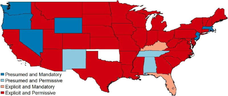
Alaska and Washington D.C. are both explicit and permissive, and Hawaii is explicit and mandatory. Oklahoma has no data. Data source is the NABP Survey of Pharmacy Laws (2006-2012).

TABLE 2.

State generic substitution laws

2006
	Mandatory	Permissive
Presumed consent	7	3
Explicit consent	3	37
2012
	Mandatory	Permissive
Presumed consent	5	7
Explicit consent	6	32

Data on state regulations is taken from the Survey of Pharmacy Laws, for 49 states and Washington, DC.

TABLE 3.

US generic substitution policy changes between 2006 and 2012

Year	Policy change	State(s)
2008	Mandatory to permissive	Minnesota, Mississippi, New York, Pennsylvania, West Virginia
2009	Permissive to mandatory	Oregon, Wyoming
2009	Presumed to explicit consent	Alabama
2009	Explicit to presumed consent	Illinois
2012	Explicit to presumed consent	Michigan
2012	Permissive to mandatory	Hawaii

Data on state regulations is taken from the Survey of Pharmacy Laws.

2.2 Data

Our data on drug consumption come from the household and prescribed medicine components of the Medicare Expenditure Panel Survey (MEPS), and includes the years 2006-2012 (AHRQ 2006-2012). The average patient-level characteristics in states under each policy are reported in Table 4. Across both types of law, the demographic characteristics of the individuals are relatively similar.

TABLE 4.

Demographic characteristics of patients

	States with explicit consent	States with presumed consent
Male	0.41	0.42
White	0.77	0.80
Black	0.16	0.13
Age	57.2	55.8
Medicare	0.24	0.20
Medicaid	0.09	0.11
Private insurance	0.28	0.32
Other insurance	0.10	0.09
Uninsured	0.28	0.27
N	12,130	2,180
	States with permissive substitution law	States with mandatory substitution law
Male	0.41	0.40
White	0.78	0.77
Black	0.16	0.16
Age	56.8	57.5
Medicare	0.23	0.25
Medicaid	0.09	0.11
Private insurance	0.29	0.27
Other insurance	0.10	0.10
Uninsured	0.29	0.27
N	10,340	3,970

Characteristics of the individuals in the difference-in-differences analytic sample using MEPS data.

We focus on three types of drugs: statins, antidepressants, and proton pump inhibitors (PPIs). These drugs are used to reduce cholesterol, treat depression, and reduce gastric acid production, respectively. Statins and antidepressants were selected because heart disease and mental disorders are among the three most costly conditions in the U.S., according to the MEPS data (Soni 2008). We add PPIs to the sample to examine how the effects of the laws vary across drugs that treat conditions of varying severity. Table 5 presents each of the drugs examined, with its generic name, brand name, and corresponding years of availability. All nine drugs had generic counterparts available between 2006 and 2012.

TABLE 5.

Drug information

	Antidepressants (SSRIs)
Generic name	Fluoxetine	Paroxetine	Citalopram	Sertraline	Escitalopram
Brand name	Prozac	Paxil	Celexa	Zoloft	Lexapro
Year brand available	1987	1992	1998	1991	2002
Year generic available	2001	2003	2004	2006	2012
	PPIs
Generic name	Lansoprazole	Omeprazole
Brand name	Prevacid	Prilosec
Year brand available	1995	1989
Year generic available	2009	2002
	Statins
Generic name	Pravastatin	Simvastatin
Brand name	Pravachol	Zocor
Year brand available	1991	1992
Year generic available	2006	2006

SSRIs are selective serotonin reuptake inhibitors. The year of drug availability is obtained from the date of FDA approval.

Figure 2 shows how the generic drugs’ market shares evolved in the years of the sample, based on quantities of tablets purchased for each drug in each year. All nine generic drugs show an upward trend. For the five branded drugs that lost patent protection between 2006 and 2012, their generic counterparts’ shares rose quickly from around 20 percent in the first year of availability to around 80 percent in 2012.

Figure 2. Generic drug share evolution, 2006–2012.

Source: MEPS baseline sample

Table 6 presents information on the average out-of-pocket payment (OPP) of one tablet of each drug in its most common strength, under different insurance statuses. As expected, the generic drugs are substantially cheaper for consumers. Generic drugs cost only 32 percent of the price of their brand name counterparts. Medicaid beneficiaries pay the least out-of-pocket for prescription drugs on average, followed by Medicare, private insurance, and no insurance. Additionally, the difference between the brand and generic OPP is much more pronounced in private insurance than Medicaid or Medicare. This is the result of the institutional features of Medicaid and Medicare, which both encourage generic drug uptake through their formularies, rather than OPP incentives.

TABLE 6.

Average out-of-pocket payment (OPP) and total payment for one tablet of selected drugs

Drug name and strength	Brand/Generic	OPP	Total payment	OPP, private insurance	OPP, Medicaid	OPP, Medicare	OPP, no insurance
Anti-Depressants
Prozac 20 mg	Brand	0.82	2.98	0.27	0.06	0.84	1.94
Fluoxetine 20 mg	Generic	0.36	0.90	0.25	0.02	0.09	0.76
Paxil 20 mg	Brand	0.80	1.69	0.52	0.09	0.10	1.43
Paroxetine 20 mg	Generic	0.26	0.83	0.30	0.03	0.09	0.50
Zoloft 100 mg	Brand	1.11	2.30	0.67	0.10	0.32	2.51
Sertraline 100 mg	Generic	0.24	0.78	0.24	0.05	0.12	0.52
Celexa 20 mg	Brand	0.64	1.66	0.61	0.08	0.20	1.73
Citalopram 20 mg	Generic	0.23	0.59	0.25	0.04	0.11	0.36
Lexapro 20 mg	Brand	1.30	4.32	1.44	0.04	0.45	3.90
Escitalopram 20 mg	Generic	0.40	3.19	0.46	0.08	0.36	0.65
PPIs
Prevacid 30 mg	Brand	1.09	5.50	0.84	0.03	0.48	5.74
Lansoprazole 30 mg	Generic	0.35	2.27	0.27	0.02	0.21	1.72
Prilosec 20 mg	Brand	0.42	1.24	0.32	0.03	0.14	1.63
Omeprazole 20 mg	Generic	0.31	1.13	0.23	0.06	0.12	1.11
Statins
Pravachol 40 mg	Brand	1.24	3.58	0.51	0.02	0.50	3.43
Pravastatin 40 mg	Generic	0.23	0.74	0.19	0.04	0.11	0.44
Zocor 20 mg	Brand	1.18	3.59	0.44	0.05	0.29	4.55
Simvastatin 20 mg	Generic	0.27	0.91	0.22	0.04	0.14	0.62
All
All brand name drugs		0.95	2.99	0.62	0.06	0.37	2.98
All generic drugs		0.29	1.26	0.27	0.04	0.15	0.74
Average difference between brand and generic		0.66	1.73	0.36	0.01	0.22	2.24

The out-of-pocket payment (OPP) and total payment are calculated for a purchase of one tablet of each drug’s most common strength using MEPS data in the years 2006-2012.

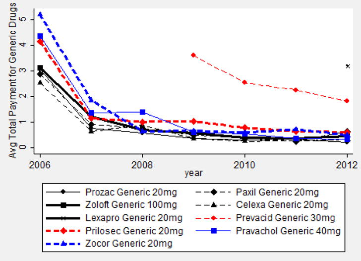
The prices for both generics and brand name drugs moved relatively smoothly across the years of the sample, except for from 2006 to 2007, when all drugs saw reductions in copayments and total payments (see Figure A1, A2, A3, and A4, in the Appendix). The drop can be mostly attributed to the introduction of Medicare Part D in 2006, which reduced pharmaceutical prices by 25 percent (Duggan and Morton 2010).

To select our sample, we begin with the 2,188,198 prescription medicine events in the MEPS sample from 2006-2012. After restricting to the nine drugs of interest, in the years that both the generic and brand name were available, and removing observations with missing or inaccurate information, 141,592 events remain in the analytic sample.

3. ANALYSES – DIFFERENCE-IN-DIFFERENCES

3.1 Methods

We use two methods to assess the effects of state drug substation laws: difference-in-differences, and a discrete choice model. The discrete choice model will be presented in Section 4. The base difference-in-differences specification is as follows:

$$\mathit{Bran}{d}_{\mathit{ijt}}={\alpha }_1\mathit{Presumed}\_\mathit{Consen}{t}_{jt}+{\alpha }_2\mathit{Mandator}{y}_{jt}+\beta x_{it}+{\alpha }_3\mathit{Yea}{r}_t+{\alpha }_4\mathit{Stat}{e}_j+{\epsilon }_{\mathit{ijt}}$$

where the dependent variable is an indicator for if the prescription drug purchase by individual i in state j and year t is a brand name drug. Presumed_Consent_jt is an indicator for an active presumed consent policy, and Mandatory_jt is an indicator for an active mandatory substitution law. Consumer characteristics, including age, sex, race, wage quartiles, and insurance status, are in x_it. State and year fixed effects are included, and standard errors are clustered at the state level. The specification above does not use the traditional difference-in-difference model design, because the policy changes occur at different times in each state. Accordingly, we are following Bertrand, Duflo, and Mullainathan (2004), Hansen (2007), and Imbens and Wooldrige (2009) to estimate a generalized difference-in-difference model. The difference-in-differences analysis is first run separately on all nine drugs in the three drug categories, then pooled for all nine drugs.

3.2 Results

The difference-in-differences regression results for individual drugs are reported in Table 7, and the pooled results are in Table 8. In Table 7, the coefficient of the presumed consent law variable is negative and significant in six of the nine individual drug regressions. For example, in the Pravachol results, the coefficient of −0.097 implies that the presumed consent law reduces the probability of purchasing brand name Pravachol, rather than generic pravastatin, by about ten percentage points. In comparison, the coefficients for the mandatory substitution law are not significantly different from zero.

TABLE 7.

Effects of state pharmacist regulations on use of specific brand name drugs, compared to their generic equivalent

Antidepressants
	Prozac	Paxil	Zoloft	Celexa	Lexapro
Presumed consent	−0.098**	−0.053**	0.066	−0.034**	−0.021***
	(0.037)	(0.026)	(0.039)	(0.013)	(0.007)
Mandatory substitution	0.131	−0.047	0.061	−0.021	0.417
	(0.084)	(0.044)	(0.038)	(0.041)	(0.264)
Dependent variable mean	0.179	0.190	0.288	0.081	0.392
Observations	11,549	9,273	15,272	12,061	826
R squared	0.12	0.21	0.33	0.14	0.29
PPIs
	Prevacid	Prilosec
Presumed consent	−0.007	−0.044**
	(0.058)	(0.017)
Mandatory substitution	−0.065	−0.053
	(0.089)	(0.068)
Dependent variable mean	0.622	0.164
Observations	2,959	26,666
R squared	0.56	0.15
Statins
	Pravachol	Zocor
Presumed consent	−0.097**	−0.009
	(0.041)	(0.012)
Mandatory substitution	0.030	−0.031
	(0.055)	(0.025)
Dependent variable mean	0.135	0.097
Observations	12,673	50,313
R squared	0.37	0.31

Difference-in-differences results from nine different regressions, using event level drug utilization data from MEPS. Dependent variable is an indicator for is the drug in question was a brand name, rather than its generic bioequivalent. All regressions feature state and year fixed effects, as well as controls for patient’s race, wage quartiles, sex, age, and insurance status. Clustered standard errors shown in parentheses.

^*p<0.1,

^**p<0.01,

^***p<0.001

TABLE 8.

Effects of state pharmacist regulations on the use of ten brand name drugs, compared to generic drug equivalents

	Baseline	Anti-depressants	PPIs	Statins	Explicit to presumed	Presumed to explicit
Presumed consent	−0.032***	−0.030**	−0.034*	−0.022***	−0.041***	−0.017*
	(0.015)	(0.013)	(0.018)	(0.008)	(0.009)	(0.009)
Mandatory substitution	−0.001	0.038	−0.036	−0.022	−0.001	0.001
	(0.025)	(0.030)	(0.080)	(0.019)	(0.025)	(0.006)
Dependent variable mean	0.158	0.194	0.210	0.105	0.167	0.166
Observations	141,592	48,981	29,625	62,986	114,681	122,598
R squared	0.16	0.14	0.13	0.31	0.16	0.16

Difference-in-differences regression results, using event level drug utilization data for antidepressants, PPIs, and statins from MEPS. Dependent variable is an indicator for if the prescription was for a brand name drug, rather than its generic bioequivalent. All regressions feature state and year fixed effects, as well as controls for patient’s race, sex, age, wage quartile, and insurance status. The 5th column drops states with policies that switched from presumed to explicit, and the 6th column drops states that switched from explicit to presumed. Clustered standard errors shown in parentheses.

^*p<0.1,

^**p<0.01,

^***p<0.001

Table 8 reports the results with drugs pooled in a single regression. The first column shows the baseline results for all nine drugs pooled together. The coefficient of −0.032 implies that the presumed consent law reduces the probability of purchasing a brand name drug by an average of 3.2 percentage points. Consistent with the findings in Table 7, the coefficient on mandatory substitution is not significant. This result is robust to clustered standard errors and block bootstrap procedures suggested by Bertrand et al. (2004). In the second, third, and fourth columns, we report the results restricted the sample of events for antidepressants, PPIs, and statins, respectively. These results suggest that the effect of the presumed consent law is slightly larger for antidepressants, and slightly smaller for statins.

We test if past policy history is important, by examining the symmetry of effects in policy changes between presumed and explicit consent laws. Intuitively, a history of presumed consent laws in a state could allow patients to become comfortable with the use of generics, which would diminish the likelihood that they would deny consent for a generic substitution. Therefore, a switch from presumed to explicit to presumed consent may have a smaller magnitude of effect than the opposite switch. Indeed, the empirical results, reported in columns 5 and 6 of Table 8, support this intuition. Column 5 drops the states that switched from presumed to explicit consent, therefore isolating the identifying variation to states that switched from explicit to presumed consent. The coefficient on presumed consent of 0.041 implies that this switch reduces the probability of purchasing brand name drugs by 4.1 percentage points. The effects of the opposite policy change (presumed to explicit consent) are shown in column 6. These policy changes had a weakly significant effect of a smaller magnitude, suggesting that past familiarity with generic drugs caused consumers to show minimal response to explicit consent laws.

3.3 Robustness checks

We include a number of robustness checks that show consistent effectiveness of the presumed consent policy on increasing generic substitution, and a lack of significant effect from mandatory substitution policies. Notably, these results hold in both the drug specific regressions (Table 7), and in the pooled regressions (Table 8). All regressions include state and year fixed effects, which control for state specific and year specific factors that could affect generic substitution. We also tested the inclusion of state-specific trend variables, which control for the possibility that unobserved differences in the states across time (e.g., macroeconomic trends) could have driven generic substitution behavior, rather than the laws in question. This specification, reported in the first column of Table A1, confirms the baseline results.

As a falsification test, we test the effects of the two laws on over-the-counter (OTC) drugs. Since these drugs are not distributed directly by pharmacists, they are not subject to the laws that regulate pharmacists’ distribution of drugs. Therefore, a consumer’s decision to buy a brand name or generic OTC drug should not be affected by the laws. We use the same difference-in-differences specification described above to examine three OTC drugs: Claritin, Zantac, and Zyrtec.² The results of these tests, reported in the second column of Table A1, confirm that as expected, neither law has a significant effect on the use of brand name OTC drugs, rather than their generic counterparts.

In order to compare our results with the existing work of Shrank et al. (2010), we analyzed generic substitution of Zocor in a Medicaid only sample, with controls designed to match those in the earlier paper. The results are reported in the third specification of Table A1, and show a weakly significant decline of approximately 3 percentage points in the purchases of brand name Zocor caused by the presumed consent law. These results match the sign and intuition of Shrank et al.’s findings, but the magnitudes should not be compared because our analyses use difference-in-differences regressions of event-level data, and the earlier work used state-level cross-sectional comparisons.

We considered the possibility that the mandatory substitution law could be more effective in states with presumed consent laws. Table A1 column 4 reports results from regressions that include an interaction term for the presence of both laws. The coefficient has a negative magnitude, but is not statistically significant. To account for the possibility that drug diffusion rates could vary across molecule, we included year-molecule fixed effects in our measurement of the aggregate effect of the two policies. These results are presented in specification 5 of Table A1, and show that these diffusion rates do not alter our estimation of the aggregate effect of either law.

Tests of supply-side responses to policy changes

Our identification strategy requires that there are no supply-side responses to changes in the state regulations on generic drugs. For example, if pharmaceutical firms adjusted their advertising strategies in response to the law changes, our results could be driven by these responses, rather than the actual laws. However, it is well documented in the literature that prescription drugs without patent protection are rarely advertised by their manufacturers (Sinkinson and Starc 2015). Since every drug we analyzed has a generic alternative, we expect that pharmaceutical advertising changes should not affect our results.

A similar problem could exist if pharmaceutical firms adjusted their pricing strategies in response to the law changes, which would bias our results. This is a concern because our analyses aim to capture demand-side responses to the law changes, rather than any supply-side reactions. Therefore, we use MEPS data in a similar difference-in-differences strategy as in our base specifications, to assess the effects of the two laws on the total payment to firms for the nine drugs shown in Table 5. The results of are shown in Table A4, in the appendix, and show no evidence of price responses to either law. However, these results should be interpreted with care, because we do not have information on rebates from pharmaceutical firms to insurers, which are known to have a role in prescription drug prices (Herper 2012).

Robustness Checks on the Error Terms

A well-known problem with difference-in-differences estimation is serial correlation of the error term, which can cause severe over-rejection of null hypotheses (Bertrand, Duflo, and Mullainathan 2004). We address this using these authors’ approach, the details of which are in the appendix. The results confirm our base specification, as shown in Table A5.

4. ANALYSES – DISCRETE CHOICE MODEL

4.1 Model

To provide further insight on the mechanisms and explore counterfactuals of the presumed consent law, we build a discrete choice model of prescription drug choice in settings with laws requiring presumed consent, versus explicit consent. For simplicity, we focus on antidepressants. Individuals are considered to have ten pharmaceutical drug alternatives for the treatment of depression; they are the antidepressants shown in Table 6. While the concepts of this model would apply to other classes of drugs, the magnitudes of the estimated relationships might vary for a number of reasons, including differential brand loyalty patterns across drug classes and their targeted conditions. Our analytic sample includes 19,002 events in 50 states. The utility of consumer i, living in market (state) m, from the purchase of product j, is decomposed into observable and unobservable parts, as in Train (2009):

$$U_{\mathit{imj}}=V\left(p_{\mathit{imj}},x_{ij}\right)+{\epsilon }_{ij}$$

The price of a product (consumer out-of-pocket payment) varies over individuals and markets, and the product price we observe in the data is denoted $p_{\mathit{imj}}$. Other product attributes do not vary over markets. Product specific constants are included. Their interactions with consumer characteristics are denoted as $x_{ij}$. The unobserved utility is ${\epsilon }_{ij}$.

Our specification for $V(.)$ and ${\epsilon }_{ij}$ is given as:

$$U_{\mathit{imj}}={\alpha }_0{p}_{\mathit{imj}}+\beta x_{ij}+{\alpha }_1\ast \mathit{Bran}{d}_j\ast \mathit{Presumed}\_\mathit{Consen}{t}_{im}+{\epsilon }_{ij}$$

In reality, a patient’s consumption of prescription drugs is a joint decision determined by both the physician and the patient. While we cannot separately identify the preference parameters of both parties, this does not affect our estimation of the parameter of interest ${\alpha }_1$. This is because the presumed consent law only takes effect after the physician has written a prescription. Therefore, it only affects the consumer’s utility without being influenced by the physician, making our data sufficient to identify ${\alpha }_1.$

The key element of the model, ${\alpha }_1\ast \mathit{Bran}{d}_j\ast \mathit{PresumedConsen}{t}_{im}$, is an extra cost item for consumers who would like to buy a brand name drug in a state with a presumed consent law. This is based on the intuition that a policy that mandates generic drug substitution, regardless of patient preferences, can be modeled as a positive infinite cost of brand name drugs. In this case, a consumer would always choose a generic drug. Similarly, a policy with no pharmacist intervention can be modeled as having zero additional cost to purchase brand name drugs. The goal of the model is to identify the difference in costs between the presumed and explicit consent policies, both of which lie between the extremes presented above.

In our model, the price variable, $p_{\mathit{imj}}$, is endogenous, because it is not independent of ${\epsilon }_{ij}$ (Villas-Boas and Winer 1999, Petrin and Train 2010). We address this problem with the control function approach, which derives a proxy variable that conditions on the portion of $p_{\mathit{imj}}$ that depends on ${\epsilon }_{ij}$. Then, the remaining variation in the endogenous variable will be independent of the error term, and standard estimation techniques will be consistent. The endogenous price $p_{\mathit{imj}}$ can be written as a function of all exogenous variables entering utility of any other choices, denoted $x_{mj}$; the variables $z_{mj}$, that do not enter utility directly but that do impact $p_{\mathit{imj}}$; and unobserved terms ${\mu }_{mj}$:

$$p_{\mathit{imj}}=W\left(x_{mj},z_{mj},{\mu }_{mj}\right)$$

The approach maintains that ${\epsilon }_{\mathit{imj}}$ and ${\mu }_{mj}$ are independent of $x_{mj}$ and $z_{mj}$, but not independent of each other. This equation illustrates the source of dependence between $p_{\mathit{imj}}$ and ${\epsilon }_{\mathit{imj}}$, as ${\mu }_{mj}$ impacts $p_{\mathit{imj}}$, but is not independent of ${\epsilon }_{\mathit{imj}}$. The key to the control function is that, under the maintained assumptions, conditional on ${\mu }_{mj}$, ${\epsilon }_{\mathit{imj}}$ is independent of $p_{\mathit{imj}}$. Decomposing ${\epsilon }_{\mathit{imj}}$ into the part that can be explained by a general function of ${\mu }_{mj}$ and the residual yields:

$${\epsilon }_{\mathit{imj}}=CF\left({\mu }_{mj};\lambda \right)+\stackrel{\sim }{{\epsilon }_{\mathit{imj}}}$$

where $CF\left({\mu }_{mj};\lambda \right)$ denotes the control function with parameters $\lambda$. As in Train (2009), we specify the control function as linear in ${\mu }_{mj}$, and the utility is given as

$$U_{\mathit{imj}}=V\left(p_{\mathit{imj}},x_{ij}\right)+\lambda {\mu }_{mj}+\stackrel{\sim }{{\epsilon }_{\mathit{imj}}}$$

With this specification, the probability that consumer $i$ chooses product $j$ is equal to

$$P_{ij}=\int I(U_{ij}>U_{il}\forall j\ne l)f\left({\beta }_i,\stackrel{\sim }{{\epsilon }_{\mathit{imj}}}\right)d{\beta }_{i}d\stackrel{\sim }{{\epsilon }_{\mathit{imj}}}$$

In order to complete the specification, we assume that β is distributed normally, and that ε is distributed logistically. We allow consumers to have heterogeneous preferences in price and brand loyalty. The log-likelihood function is:

$$LL\left(\beta ,\alpha \right)={\sum }_{i=1}^I{\sum }_j{y}_{ij}\text{ln}\left(P_{ij}\right)$$

The specification is easily generalized to allow for repeated choices by each sampled decision maker (Train 2009). In the estimation section below, we show results with and without considering the panel design of the data.

4.2 Consumer Choice Model Estimation and Results

The model is estimated in two steps. First, the endogenous variable, out-of-pocket payment (OPP), is regressed on observed choice characteristics and the instruments. Second, the choice model is estimated with the predicted residuals from the first step entering as an extra variable.

As an instrument for OPP, we use the number of firms producing the molecule in each market. This measure of competition intensity is strongly correlated with market price (and OPP) and therefore constitutes a strong instrument. To satisfy the exclusion restriction, the number of firms should not be correlated with drug purchase decisions, except through its effect on OPP. While this assumption may not be valid in a multi-class analysis, we believe that is accurate within the SSRIs, where selection between molecules is primarily determined by formularies. Our instrument, the number of firms producing the drug in the market, has a negative and highly significant association with OPP, as expected. As a robustness check, we tested a second instrument, the average OPP of the product in other markets, as suggested by Petrin and Train (2010). This instrument yielded similar results. We also used this second instrument to perform an over-identification test on the first instrument, which confirmed the validity of our main instrument.

The multinomial logit model requires OPP information for all possible product choices of consumers. However, in the data, we only observe the OPP of their consumption choice. Therefore, we impute the OPP for all the products that they did not purchase, using the average OPP for a month’s supply among consumers in the same state, year, and insurance status. This is a similar procedure to that used by Dunn (2012). Even for the product that was actually purchased, we use the imputed OPP, not the original OPP. We do not differentiate between first purchase and refill, because the presumed consent law is applied identically in both situations. The model is estimated by simulated method of likelihood (Train 2009).

The consumer choice model estimation results are presented in Table 9. Column 1, which does not instrument for OPP, shows a positive coefficient for OPP, which suggests an unreasonable upward sloping demand curve. This reflects the endogeneity of OPP, as explained in the preceding section. In column 2, we instrument for OPP with the control function approach, allow for repeated choices by the same decision maker, and allow consumers to have heterogeneous preferences across OPP, brand loyalty, and brand specific constants. These changes improve the model fit, with the log-likelihood increasing from −35,895 to −19,685. After instrumenting, the OPP coefficient changes to a more reasonable estimate, −0.0461. The coefficient for brand is 0.4498, confirming the brand premium found in other papers. These results also suggest that older and male customers are less likely to buy brand name drugs. The significance of the alternative specific constants suggests that consumers have different preferences across antidepressants, as expected. The coefficient for the interaction between brand name drug and presumed consent is −0.1381. The ratio of this interaction coefficient to the OPP coefficient indicates that the effect of the presumed consent law on brand name antidepressants is equivalent to a $3.00 increase in their OPP.

TABLE 9.

Mixed logit estimation results for antidepressant choice, with control function approach to instrument out-of-pocket payment (OPP)

Independent variable	Without control function	With control function
Brand * presumed consent	−0.1807***	−0.1381***
	(0.0436)	(0.0483)
Years available	0.0488***	0.2750***
	(0.0037)	(0.0118)
Brand * years available	−0.1628***	−0.2425***
	(0.0041)	(0.0083)
Brand * age	−0.0078***	−0.0099***
	(0.0009)	(0.0009)
Brand * male	−0.1435***	−0.2430***
	(0.0350)	(0.0387)
Brand * white	0.0243	0.0249
	(0.0762)	(0.0847)
Brand * black	−0.1804	−0.2260
	(0.0916)	(0.1013)
Average OPP	0.0016***	−0.0461***
	(0.0003)	(0.0032)
Brand name	1.2508***	0.4498***
	(0.0993)	(0.1481)
Prozac		−31.0600***
		(7.0400)
Paxil		−6.7820***
		(1.4491)
Zoloft		−2.9010***
		(0.4450)
Celexa		−1.9245***
		(0.0751)
1st stage coefficient		−1.5500***
		(0.0468)
Observations	19,002	19,002
Log-likelihood	−35895	−19685

Results of mixed logit regressions for choice of five antidepressants shown in Table 5. In column 2, OPP is instrumented with the number of firms producing each drug in that market. Column 2 allows repeated purchases by consumers, and heterogeneous preference across drugs. Standard errors are clustered the state level. All specifications include controls for the standard deviation of average OPP, and brand name. Column 2 also includes variables the standard deviations of the molecule variables.

^*p<0.1,

^**p<0.05,

^***p<0.01

Since the model above is non-linear, we cannot directly interpret the impact of the presumed consent law based on the sign and magnitude of the coefficients reported above. To ease interpretation, we calculate the average marginal effects on antidepressant choice of all states switching from an explicit to presumed patient consent law. The results are presented in Table 10. We see that switching to presumed consent reduces the average probability of purchasing the brand name version of a drug by approximately six to eleven percent.

TABLE 10.

Average marginal effect of change in consent law

Drug type	Predicted probability of purchase under explicit consent	Predicted probability of purchase under presumed consent	Percent change from explicit to presumed consent
Prozac	0.0207	0.0233	−12.56%
Fluoxetine	0.1846	0.1818	1.52%
Paxil	0.026	0.0286	−10.00%
Paroxetine	0.1215	0.1182	2.72%
Zoloft	0.0863	0.093	−7.76%
Sertraline	0.1769	0.1696	4.13%
Celexa	0.0245	0.026	−6.12%
Citalopram	0.1878	0.1774	5.54%
Lexapro	0.1746	0.1863	−6.70%
Escitalopram	0.0794	0.0772	2.77%

The predicted probabilities of purchasing drugs are calculated based on the mixed logit model specified in column 2 of Table 10.

It is critical that the estimated choice model predicts reasonable product substitution patterns. Our model predicts that the price elasticity ranges from −0.005 to −0.09, which is smaller than estimates found in recent literature (Simonsen, Skipper, and Skipper 2016). The differences most likely stem from our model specification, which calculates the price elasticity conditional on purchase. Adding an outside option of not purchasing would result in higher estimates of the price elasticities. Also, our model exhibits significant within molecule substitution. When the OPP of a brand name drug increases by one percent, the majority of the consumers who switch choose to stay with the same molecule.

5. DISCUSSION

5.1 Interpretation of the Difference-in-Differences Results

The results from both difference-in-differences and the discrete choice model analyses suggest that the presumed consent law increases the use of generic drugs, compared to explicit consent laws. There was no evidence, however, of an effect from the mandatory substitution laws. This seems counterintuitive, because we expect a policy that mandates generic substitution to increase the use of generics.

The differential effectiveness of the two laws is likely explained by the nature of pharmacist revenues and costs, which create larger profit margin on generic drugs (Boehm et al. 2013, CBO 1998). Indeed, gross profit dollars are approximately 50 percent higher for generic drugs than for brand name drugs (Trefis Team 2013). As a result of market imperfections, pharmacists have advantages in both revenue and costs when dispensing generic drugs, compared to brand name drugs. This explains the lack of observed effects of the mandatory substitution law in our results; pharmacists have a strong incentive to substitute generic for brand name drugs, regardless of whether the state has a mandatory or permissive substitution law. The presence of a presumed consent law, on the other hand, alters the default choices given to consumers, rather than pharmacists, and therefore its effects would not be influenced by pharmacist profit incentives. For a full description of the market imperfections that affect both pharmacist generic drug revenue and decrease costs, please see the appendix.

Furthermore, the effectiveness of the presumed consent law is logical, given evidence that documents the difficulty of changing consumer’s preferences for branded products (Ling, Berndt, and Kyle 2002, Beshears et al. 2013, Carrera and Villas-Boas 2013). When explicit patient consent is required, the patient is given a clear chance to persist with their preference, rather than substitute, as the pharmacist and payer of the drug costs would have wanted them to do.

Our results showed different effects of the presumed consent law across drugs. Antidepressants appear to have been more affected by the law than statins. One reason for this could be that statins have well-known side effects on hepatic and skeletal muscle toxicity, which caused consumers and physicians to exert more brand loyalty than for other types of drugs (Chong, Seeger, and Franklin 2001). The same loyalty distortion could also be caused by direct-to-consumer advertising or detailing for brand name statins. These same perceptions from consumers and physicians about relative generic quality could also be part of the reason why effects varied across molecules. Another possibility is that other external factors, not captured in our model, increased the popularity of these brands in concordance with the policy changes.

To further examine differences in effectiveness across consumer type, we ran the difference-in-differences regressions on several restricted samples. In one test, we compared the effects of the laws in events where users had previous generic use, to the effects in the events where users had previous branded drug use. The results are reported in the first and second specification of Table A2, and show that in brand experience events, the presumed consent law decreased the probability of purchasing a branded drug by approximately 15 percentage point, compared to a 1 percentage point decrease in generic experience events. This fits with the intuition that those already comfortable with generics are less susceptible to the effects of the presumed consent law. We also split the sample by insurance status, and reported the results in specifications 6-9 of Table A1. We see that the presumed consent law has larger average effects for the privately insured and Medicare, although the effects for Medicare were not statistically significant. The presumed consent law had insignificant effects for Medicaid, and nearly a zero effect for the uninsured. The lack of effect for the uninsured may possibly reflect that this group would rarely have ever bought brand name drugs to begin with, leaving little margin for effectiveness of the law.

Finally, we tested if the effects of the laws were symmetric. The directionality of the presumed consent law was explained at the end of section 3.2, and those results were presented in Table 8. The symmetry of the mandatory substitution law was tested with similar methodology, and the results are presented in specifications 3 and 4 of Table A3. Regardless of the direction of these policy changes, the mandatory substitution has an insignificant effect on generic substitution. Additionally, we tested directionality of the policy changes in the experience-defined subsamples that are explained in the previous paragraph, and the results fit with the previously discussed intuition (Table A3, specifications 5-12).

5.2 Mechanisms of the Presumed Consent Law

In the consumer choice model above, the presumed consent law is modeled as an extra cost to buy brand name drugs. This impact, captured parsimoniously, could be occurring through several behavioral channels. The first possible channel stems from consumer’s inattention. Under the presumed consent law, substitution is only noted on the label of the prescribed drugs, making it possible that the consumers do not notice the substitution. It has been well documented that limited attention affects consumer decisions under various scenarios, including the timing of earnings announcements affecting investment decisions, and effects of tax-inclusive prices on alcohol purchases (DellaVigna and Pollet 2009, Chetty, Looney, and Kroft 2009).

Another possible source of the presumed consent law’s impact is dynamic preference inconsistency. For instance, a consumer might notice the switch, and decide to go to the pharmacist the next day to ask for a brand, but never follow through with these intentions. Finally, it is possible that the cost parameter is capturing a switching cost, which is the effort of asking the pharmacists to switch back to brand name drugs. Our model does not try to differentiate among these possible behavioral channels. Rather, the extra cost parameter in the choice model is meant to capture the aggregate impact of these channels.

5.3 Limitations

In order for our analyses to be interpreted as causal, the changes in the drug substitution laws between 2006 and 2012 must have been exogenous. But, as Besley and Case (2000) pointed out, state policy making could be endogenous, perhaps as a response to economic and political conditions within a state. In order to evaluate the validity of our causal conclusions, we consider the reasoning behind the policy changes that constitute our identifying variation.

Information on the motivations for the specific state policies used in this paper is scarce, but another type of drug substitution, between biologics and biosimilars, has received substantial media attention.³ The most common motivation for law changes in this area is political lobbying by interested parties, including pharmaceutical firms attempting to limit opportunities for substitution (Pollack 2013). In addition to brand name manufacturers, other parties can be expected to have a strong lobbying interest, including generic manufacturers, insurance companies, managed care organizations, and chain pharmacies.

Given the strong influence of lobbyists in the creation of related laws for biosimilar substitution, it is reasonable that political lobbying would also exert influence on the policy changes for generic substitution that are featured in this paper. The causal conclusions of this paper could be jeopardized if lobbyists somehow influenced generic substitution through a channel other than the two laws assessed in our paper. This could potentially occur via contemporaneous policy changes in regulations on physicians’ power to forbid substitution, or in state formulary regulations. The Survey of Pharmacy Laws reveals that three states changed the regulations on physicians’ power to forbid substitution in the years 2006-2012, but these changes were quite minor.⁴ Additionally, these physician requests only occur in a small portion of prescriptions (Shrank et al. 2011). Therefore, we believe that these changes did not bias our results. The other concern is if state formulary regulations changed during the years of the study. The formulary definitions changed in Delaware and Missouri during our sample, but neither affected any of the nine molecules in the study, and thus do not confound our analyses.

Another concern is the possibility that insurance companies either influenced or reacted to the policy changes, in which case our results could be driven by consumer responses to insurance changes, rather than the actual policy changes. We deal with this possibility by controlling for insurance status in all specifications, and controlling for drug costs in the mixed logit regressions. Additionally, we examined the trends of Medicare payments, Medicaid payments, and out-of-pocket costs around the time of the policy changes in the three states that switched between presumed and explicit consent (Alabama, Illinois, and Michigan). We found that the insurers in these states behaved similar to the rest of the nation, suggesting that the insurers did not influence or react to the policy changes in those states. Other limitations of our study include the relatively short period of our panel (2006-2012), and the limited number of policy changes that occurred during this period.

6. CONCLUSION

Prescription drugs are a large and growing portion of health expenditures. Increasing the use of generic drugs, rather than bioequivalent brand name drugs, is a promising option for controlling spending growth in this sector of health care. This study assesses the effectiveness of two different state policies that regulate pharmacists’ substitution of generic drugs for bioequivalent brand name drugs. Results from difference-in-difference regressions show that when pharmacists do not need to acquire explicit consent from patient for substitution, they are 3.2 percentage points more likely to dispense a generic drug. In a back of the envelope calculation, we estimate that if the 39 remaining explicit consent states switched to presumed consent, total prescription drug spending in those states would be reduced from $297 billion to $246 billion (see appendix for details). Another type of policy, which mandates generic substitution by pharmacists (unless overruled by the patient), was found to have an insignificant effect. This is most likely because pharmacists have a profit incentive to substitute generics, regardless of that policy. The presumed consent law, on the other hand, affects consumers’ observed choice set, and is therefore unrelated to pharmacist incentives. A discrete choice model suggests that the presumed consent law has a similar effect on consumption of brand name drugs as a three dollar increase in the price of these drugs. Our findings have important policy implications, because they inform efforts to increase the use of generic drugs, which are much less expensive than their brand name equivalents.

APPENDIX

Examples of the mandatory and permissive substitution laws

An example of a mandatory substitution law is the legislation in Florida: “A pharmacist who receives a prescription for a brand name drug shall, unless requested otherwise by the purchaser, substitute a less expensive, generically equivalent drug product,” (Florida Legislature, 2016). An example of a permissive substitution law is the Illinois legislation: “A brand name or non-brand name drug product of the same generic name may be dispensed by the pharmacist, provided that the selected drug has a unit price less than the drug product specified in the prescription,” (Illinois Legislature, 2016).

Examples of the explicit and presumed consent laws

An example of an explicit consent law is the Pennsylvania regulation: “Any pharmacist who substitutes any drug shall notify the person presenting the prescription of such substitution together with the amount of the retail price difference between the brand name and the drug substituted for it and shall inform the person presenting the prescription that they may refuse the substitution,” (Pennsylvania Legislature, 2016). An example of a presumed consent law, from Massachusetts, merely requires notification of the substitution on the label: “The pharmacist shall indicate on the label in the following manner the fact of the interchange: ‘Interchange: (name of exact drug product dispensed’,” (Massachusetts Legislature, 2016).

Bertrand, Duflo, and Mullainathan’s procedure for dealing serial correlation of the error term

A well-known problem with difference-in-differences estimation is serial correlation of the error term, which can cause severe over-rejection of null hypotheses (Bertrand, Duflo, and Mullainathan 2004). One solution to this problem is to use block bootstrap, aggregate the time periods, or use unrestricted variance-covariance matrices to overcome the serial correlation problem. Since the policy changes are staggered, however, we cannot simply aggregate the time periods and run a two period difference-in-differences regression. Instead, we follow Bertrand, Duflo, and Mullainathan’s (2004) approach. First, we regress the dependent variable on state fixed effects, year dummies, and any relevant covariates. Then, we divide the residuals of the treatment group states into two groups: residuals from years before the laws were changed, and residuals from years after the law changes. The estimate of the laws’ effect and its standard error can then be obtained from an OLS regression in this two-period panel. This procedure is comparable to the simple aggregation of time periods for laws that are passed for the entire treatment group at the same time. We found similar effects and the regression results are presented in Table A5 in the appendix.

Description of pharmacist revenues and costs for generic drugs

Market imperfections affect both pharmacy costs and revenue, which leads to greater pharmacy profits when dispensing generics (Boehm et al. 2013, CBO 1998). Pharmacies are almost always paid by third party insurers for prescription drugs. The insurance payments to pharmacies (i.e. pharmacy revenue) are based on a benchmark price called the average wholesale price (AWP). The AWP is reported by generic producers themselves, and until recently has been subject to essentially no independent verification. As a result, generic manufacturers have an incentive to compete for market share by reporting AWPs that exceed actual average wholesale prices. This “spread” drives up pharmacy revenue, increasing their profits, and makes pharmacies more likely to stock the products of that manufacturer. Indeed, gross profit dollars are approximately 50 percent higher for generic drugs than for brand name drugs (Trefis Team 2013). Accordingly, pharmacists respond to the incentives inherent in AWP-based reimbursement by opting to dispense these drugs whenever possible (Alpert, Duggan, and Hellerstein 2013). In addition to the inflated revenues of generic dispensing described above, pharmacists also experience a cost advantage when purchasing generic drugs rather than brand name. This is because pharmacists have greater bargaining power in price negotiations with generic manufacturers, who often have several competitors. Brand name manufacturers, enjoying their patent protected monopoly, exploit their own bargaining power to drive down the pharmacist profit margins on brand name drugs.

Estimation of savings that would occur with nationwide adoption of presumed consent policies in the United States

In 2016, $297 billion was spent on prescription drugs in the 39 explicit consent states (Kaiser Family Foundation, 2017). Of this total amount, 15% ($45 billion) was spent on generics (for 84.6% of fills), and 85% ($252 billion) was spent on branded drugs (for 15.4% of fills) (Quintiles IMS Institute, 2017). If these states switched to presumed consent, it would increase their generic use rate by 3.2 percentage points, from 84.6% to 87.8%. The associated reduction in spending, assuming no change in aggregate drug consumption in those states, would result in a net reduction in prescription drug spending of approximately $51 billion.

Figure A1. Average out-of-pocket payment for brand name drugs.

Source: MEPS baseline sample

Figure A2. Average out-of-pocket payment for generic drugs.

Source: MEPS baseline sample

Figure A3. Average total payment for brand name drugs.

Source: MEPS baseline sample

Figure A4. Average total payment for generic drugs.

Source: MEPS baseline sample

TABLE A1.

Robustness checks with additional specifications and insurance status restrictions

	1	2	3	4	5
	State specific trends	OTC drugs	Zocor in Medicaid	Law interactions	Year-molecule fixed effects
Presumed consent	−0.033***	0.063	−0.027*	−0.032***	−0.029***
	(0.011)	(0.050)	(0.014)	(0.012)	(0.007)
Mandatory substitution	−0.016	0.094		0.002	0.003
	(0.031)	(0.094)		(0.029)	(0.023)
Presumed consent *				−0.021	−0.008
Mandatory substitution				(0.015)	(0.052)
Dependent variable mean	0.158	0.257	0.080	0.158	0.158
Observations	141,592	5,630	3,556	141,592	141,592
R squared	0.17	0.40	0.53	0.16	0.27
	6	7	8	9
	Medicare	Medicaid	Private insurance	Uninsured
Presumed consent	−0.065	0.046	−0.037***	−0.020
	(0.046)	(0.039)	(0.009)	(0.018)
Mandatory substitution	0.023	0.063	−0.018	−0.041
	(0.043)	(0.039)	(0.027)	(0.039)
Dependent variable mean	0.129	0.197	0.199	0.118
Observations	41,510	13,498	36,736	36,393
R squared	0.17	0.17	0.14	0.28

Difference-in-differences regression results, using event level drug utilization data from MEPS. Dependent variable is an indicator for if the prescription was for a brand name drug, rather than its generic bioequivalent. All regressions feature state and year fixed effects, as well as controls for patient’s race, sex, age, wage quartiles, and insurance status, except column 3, which includes only year fixed effects. Column 3 is designed to replicate Shrank et al (2010). Column 1 includes state specific trends. Column 5 also includes year-molecule fixed effects. Clustered standard errors shown in parentheses.

^*p<0.1,

^**p<0.01,

^***p<0.001

TABLE A2.

Sample restrictions based on drug use experience, with additional controls

	1	2
	Generic experience	Brand experience
Presumed consent	−0.009**	−0.152***
	(0.004)	(0.033)
Mandatory substitution	0.018	0.071
	(0.011)	(0.054)
Dependent variable mean	0.050	0.720
Observations	108,085	28,672
R squared	0.05	0.07
	3	4
	Generic experience	Brand experience
Presumed consent	−0.011**	−0.168***
	(0.005)	(0.025)
Mandatory substitution	0.010	0.070
	(0.013)	(0.052)
Presumed consent * Mandatory substitution	0.041	0.004
	(0.025)	(0.076)
Dependent variable mean	0.050	0.720
Observations	108,085	28,672
R squared	0.05	0.07
	5	6
	Generic experience	Brand experience
Presumed consent	−0.008**	−0.154***
	(0.004)	(0.047)
Mandatory substitution	0.016	0.066
	(0.011)	(0.043)
Dependent variable mean	0.050	0.720
Year-molecule fixed effects	X	X
Observations	108,085	28,672
R squared	0.14	0.13

Difference-in-differences regression results, using event level drug utilization data from MEPS. Dependent variable is an indicator for if the prescription was for a brand name drug, rather than its generic bioequivalent. All regressions feature state and year fixed effects, as well as controls for patient’s race, sex, age, wage quartiles, and insurance status. Experience restrictions keep only individuals with the type of drug use experience noted in the column heading. Clustered standard errors shown in parentheses.

^*p<0.1,

^**p<0.01,

^***p<0.001

TABLE A3.

Sample restrictions based on direction of law changes, with variation for drug use experience

	1	2	3	4
Policy change	Explicit to presumed	Presumed to explicit	Permissive to mandatory	Mandatory to permissive
Presumed consent	−0.041***	−0.017*	−0.031***	−0.031***
	(0.009)	(0.009)	(0.008)	(0.008)
Mandatory substitution	−0.001	0.001	0.012	−0.025
	(0.025)	(0.006)	(0.040)	(0.043)
Dependent variable mean	0.167	0.166	0.165	0.166
Observations	114,681	122,598	101,393	104,502
R squared	0.16	0.16	0.16	0.16
	5	6	7	8
Policy change	Explicit to presumed	Presumed to explicit	Permissive to mandatory	Mandatory to permissive
Experience restriction	Generic	Generic	Generic	Generic
Presumed consent	−0.014***	−0.003	−0.009***	−0.009***
	(0.008)	(0.004)	(0.007)	(0.007)
Mandatory substitution	0.017	0.017	0.034	0.048
	(0.011)	(0.012)	(0.025)	(0.033)
Dependent variable mean	0.053	0.053	0.053	0.054
Observations	106,535	99,607	88,119	90,875
R squared	0.05	0.05	0.05	0.05
	9	10	11	12
Policy change	Explicit to presumed	Presumed to explicit	Permissive to mandatory	Mandatory to permissive
Experience restriction	Brand	Brand	Brand	Brand
Presumed consent	−0.122***	−0.142***	−0.153***	−0.155***
	(0.059)	(0.023)	(0.059)	(0.058)
Mandatory substitution	0.072	0.067	−0.029	0.070
	(0.055)	(0.044)	(0.041)	(0.058)
Dependent variable mean	0.718	0.715	0.719	0.718
Observations	28,221	26,538	23,247	23,998
R squared	0.07	0.08	0.07	0.07

Difference-in-differences regression results, using event level drug utilization data from MEPS. Dependent variable is an indicator for if the prescription was for a brand name drug, rather than its generic bioequivalent. All regressions feature state and year fixed effects, as well as controls for patient’s race, sex, age, wage quartiles, and insurance status. Policy change variations drop states with switches that occurred in the opposite direction. Experience restrictions keep only individuals with the type of drug use experience noted in the column heading. Clustered standard errors shown in parentheses.

^*p<0.1,

^**p<0.01,

^***p<0.001

TABLE A4.

Pharmaceutical firms’ pricing responses to state generic substitution laws

	Total payment per tablet
Mandatory substitution	−0.027
	(0.056)
Presumed consent	−0.053
	(0.040)
Brand name	1.164***
	(0.055)
Brand name * presumed consent	0.181
	(0.315)
Brand name * mandatory substitution	0.088
	(0.245)
Dependent variable mean	1.299
Observations	141,592
R squared	0.19

Difference-in-differences regression results, using event level drug utilization data for antidepressants, PPIs, and statins from MEPS. Dependent variables are the copayment and total payment for one month’s supply of each drug. Controls are state and year fixed effects, as well as patient’s race, sex, age, wage quartile, and insurance status. Clustered standard errors shown in parentheses.

^*p<0.1,

^**p<0.01,

^***p<0.001

TABLE A5.

Robustness check on the error term

	Mandatory substitution	Presumed consent
Post	0.0055	−0.0433***
	(0.0171)	(0.0102)
Observations	3687	14915

First, we regress the dependent variable on state fixed effects, year dummies, and any relevant covariates. Then, we divide the residuals of the treatment group states into two groups: residuals from years before the laws were changed, and residuals from years after the law changes. The estimate of the laws’ effect and its standard error can then be obtained from an OLS regression in this two-period panel. Clustered standard errors shown in parentheses.

^*p<0.1,

^**p<0.01,

^***p<0.001

References

- Agency for Healthcare Research and Quality. Medical Expenditure Panel Survey. Department of Health and Human Services; Rockville, MD: 2006–2012. [Google Scholar]
- Alpert Abby, Duggan Mark, Hellerstein Judith K. Perverse reverse price competition: Average wholesale prices and Medicaid pharmaceutical spending. Journal of Public Economics. 2013;108:44–62. [Google Scholar]
- Berndt Ernst R, Aitken Murray L. Brand loyalty, generic entry and price competition in pharmaceuticals in the quarter century after the 1984 Waxman-Hatch legislation. International Journal of the Economics of Business. 2011;18(2):177–201. [Google Scholar]
- Bertrand Marianne, Duflo Esther, Mullainathan Sendhil. How Much Should We Trust Differences-in-Differences Estimates? Quarterly journal of economics. 2004;119(1):249–275. [Google Scholar]
- Beshears John, Choi James J, Laibson David, Madrian Brigitte C, Reynolds Gwendolyn. Testimonials do not convert patients from brand to generic medication. The American journal of managed care. 2013;19(9):e314. [PMC free article] [PubMed] [Google Scholar]
- Besley Timothy, Case Anne. Unnatural experiments? Estimating the incidence of endogenous policies. The Economic Journal. 2000;110(467):672–694. [Google Scholar]
- Boehm Garth, Yao Lixin, Han Liang, Zheng Qiang. Development of the generic drug industry in the US after the Hatch-Waxman Act of 1984. Acta Pharmaceutica Sinica B. 2013;3(5):297–311. [Google Scholar]
- Bronnenberg Bart J, Dube Jean-Pierre, Gentzkow Matthew, Shapiro Jesse M. Do pharmacists buy Bayer? Informed shoppers and the brand premium. Quarterly Journal of Economics. 2015;130(4):1669–1726. [Google Scholar]
- Carrera Mariana, Villas-Boas Sofia. Generic aversion and observational learning in the over-the-counter drug market. Case Western Working Paper 2013 [Google Scholar]
- Chetty Raj, Looney Adam, Kroft Kory. Salience and taxation: Theory and evidence. The American economic review. 2009;99(4):1145–1177. [Google Scholar]
- Chong Pang H, Seeger John D, Franklin Cory. Clinically relevant differences between the statins: implications for therapeutic selection. The American journal of medicine. 2001;111(5):390–400. doi: 10.1016/s0002-9343(01)00870-1. [DOI] [PubMed] [Google Scholar]
- Congressional Budget Office. How increased competition from generic drugs has affected prices and returns in the pharmaceutical industry. US Government Printing Office; 1998. [Google Scholar]
- DellaVigna Stefano, Pollet Joshua M. Investor inattention and Friday earnings announcements. The Journal of Finance. 2009;64(2):709–749. [Google Scholar]
- Duggan Mark, Morton Fiona Scott. The effect of Medicare Part D on pharmaceutical prices and utilization. The American Economic Review. 2010;100(1):590–607. doi: 10.1257/aer.100.1.590. [DOI] [PubMed] [Google Scholar]
- Dunn Abe. Drug innovations and welfare measures computed from market demand: The case of anti-cholesterol drugs. American Economic Journal: Applied Economics. 2012;4(3):167–189. [Google Scholar]
- Florida Legislature. The 2016 Florida Statutes - 465.025 Substitution of Drugs 2016 [Google Scholar]
- Hansen Christian B. Generalized least squares inference in panel and multilevel models with serial correlation and fixed effects. Journal of Econometrics. 2007;140(2):670–694. [Google Scholar]
- Herper Matthew. Inside the secret world of drug company rebates. Forbes [serial on the Internet] 2012 May 10, 2012. [Google Scholar]
- Illinois Legislature. Public Act 91-0766 - An Act Regarding Pharmaceuticals 2016 [Google Scholar]
- Imbens Guido W, Wooldridge Jeffrey M. Recent developments in the econometrics of program evaluation. Journal of economic literature. 2009;47(1):5–86. [Google Scholar]
- Kaiser Family Foundation. Total Retail Sales for Prescription Drugs Filled at Pharmacies. State Health Facts 2017 [Google Scholar]
- Kelton Christina ML, Chang Lenisa V, Kreling David H. State Medicaid programs missed $220 million in uncaptured savings as generic fluoxetine came to market, 2001–05. Health Affairs. 2013;32(7):1204–1211. doi: 10.1377/hlthaff.2013.0161. [DOI] [PubMed] [Google Scholar]
- Ling Davina C, Berndt Ernst R, Kyle Margaret K. Deregulating direct‐to‐consumer marketing of prescription drugs: effects on prescription and over‐the‐counter product sales. Journal of Law and Economics. 2002;45(S2):691–723. [Google Scholar]
- Massachusetts Legislature. Section 12D Prescriptions of interchangeable drug products; notification of substitute for narrow therapeutic index immunosuppressant drug for treatment of organ or tissue transplant 2016 [Google Scholar]
- National Association of Boards of Pharmacy. Survey of Pharmacy Law. Mount Prospect, IL: 2006–2012. [Google Scholar]
- OECD. OECD Health Statistics 2016. Paris: 2016. [Google Scholar]
- Pennsylvania Legislature. Pennsylvania Statutes Title 35 PS Health and Safety §960.3. Substitution for brand name drugs; oral prescription; notice to purchaser; refusal of substitution; prices; records; labels 2016 [Google Scholar]
- Petrin Amil, Train Kenneth. A control function approach to endogeneity in consumer choice models. Journal of marketing research. 2010;47(1):3–13. [Google Scholar]
- Pollack Andrew. Biotech firms, billions at risk, lobby states to limit generics. New York Times. 2013 January 28, 2013. [Google Scholar]
- Quintiles IMS Institute. Aitken Murray., editor. Medicines Use and Spending in the US: A Review of 2016 and Outlook to 2021. 2017 https://www.iqvia.com/institute.
- Shrank William H, Choudhry Niteesh K, Agnew-Blais Jessica, Federman Alex D, Liberman Joshua N, Liu Jun, Kesselheim Aaron S, Brookhart M Alan, Fischer Michael A. State generic substitution laws can lower drug outlays under Medicaid. Health Affairs. 2010;29(7):1383–1390. doi: 10.1377/hlthaff.2009.0424. [DOI] [PMC free article] [PubMed] [Google Scholar]
- Shrank William H, Liberman Joshua N, Fischer Michael A, Avorn Jerry, Kilabuk Elaine, Chang Andrew, Kesselheim Aaron S, Brennan Troyen A, Choudhry Niteesh K. The consequences of requesting “dispense as written”. The American journal of medicine. 2011;124(4):309–317. doi: 10.1016/j.amjmed.2010.11.020. [DOI] [PubMed] [Google Scholar]
- Simonsen Marianne, Skipper Lars, Skipper Niels. Price sensitivity of demand for prescription drugs: exploiting a regression kink design. Journal of Applied Econometrics. 2016;31(2):320–337. [Google Scholar]
- Sinkinson Michael, Starc Amanda. Ask your doctor? Direct-to-consumer advertising of pharmaceuticals. National Bureau of Economic Research; 2015. [Google Scholar]
- Soni Anita. MEPS Statistical brief# 331: top 10 most costly conditions among men and women, 2008: estimates for the US civilian noninstitutionalized adult population, age 18 and older. Rockville, MD: 2008. [Google Scholar]
- Train Kenneth E. Discrete choice methods with simulation. Cambridge university press; 2009. [Google Scholar]
- Trefis Team. CVS Fortifies Its Margins By Selling More Generic Drugs. Forbes. 2013 August 7, 2013. [Google Scholar]
- Villas-Boas J Miguel, Winer Russell S. Endogeneity in brand choice models. Management Science. 1999;45(10):1324–1338. [Google Scholar]