An EM-based semi-supervised deep learning approach for semantic segmentation of histopathological images from radical prostatectomies

Abstract

Automated Gleason grading is an important preliminary step for quantitative histopathological feature extraction. Different from the traditional task of classifying small pre-selected homogeneous regions, semantic segmentation provides pixel-wise Gleason predictions across an entire slide. Deep learning-based segmentation models can automatically learn visual semantics from data, which alleviates the need for feature engineering. However, performance of deep learning models is limited by the scarcity of large-scale fully annotated datasets, which can be both expensive and time-consuming to create. One way to address this problem is to leverage external weakly labeled datasets to augment models trained on the limited data. In this paper, we developed an expectation maximization-based approach constrained by an approximated prior distribution in order to extract useful representations from a large number of weakly labeled images generated from low-magnification annotations. This method was utilized to improve the performance of a model trained on a limited fully annotated dataset. Our semi-supervised approach trained with 135 fully annotated and 1,800 weakly annotated tiles achieved a mean Jaccard Index of 49.5% on an independent test set, which was 14% higher than the initial model trained only on the fully annotated dataset.

Graphical abstract

1. Introduction

Prostate cancer (PCa) is the most common cancer and the second leading cause of cancer death in men in United States, accounting for about 21% of newly diagnosed cancer cases, and 8% of cancer deaths (Siegel et al., 2016). The Gleason grading system, which is based on visual interpretation of tumors’ microscopic characteristics by pathologists, consists of five different histologic patterns from Gleason 1 (G1) indicating tissue that closely resembles normal prostate glands to Gleason 5 (G5) indicating the most aggressive pattern. The final Gleason score (GS) is generated by summing the most (primary Gleason pattern) and second most (secondary Gleason pattern) prevalent patterns in the tissue section. Currently, Gleason grades serve as the best biomarker in prostate cancer staging and treatment planning (Kwak et al., 2016). Patients diagnosed with high-risk PCa (GS > 7) are often treated with radical prostatectomy, radiation or hormonal therapy, while those with low-to intermediate-risk PCa (GS ≤ 7) may undergo active surveillance. Yet, a recent clinical trial showed that there is no significant difference in 10-year mortality between patients in active surveillance and treatment groups, which emphasizes the need of developing more effective biomarkers for staging and risk stratification (Hamdy et al., 2016). Moreover, manual assignment of Gleason grade is time-consuming and prone to inter- and intra- observer variability (Huang et al., 2014; Humphrey, 2004; Lavery et al., 2012).

A semantic segmentation model would provide Gleason grading for each pixel, which can be used as a preliminary step to extract quantitative pathological image features that are representative of underlying characteristics of tumor. However, training such a model may require a large-scale dataset to be annotated at gland-level, which would be expensive and time-consuming to produce. Conversely, image-level annotations extracted from low magnification annotations (LMAs) can be generated easily. Fig. 1 shows the difference between gland-level annotations and LMAs. The goal of this paper is to utilize these imagelevel annotations to adjust a classifier initially trained on a limited dataset, reducing the reliance on expensive pixel-wise annotations.

Fig. 1.

Differences between LMAs and gland-level annotations. (A) A whole slide image with LMAs visualized at 0.4×. Many weakly labeled tiles can be extracted from these LMAs. (B) A 1200 × 1200 tile sampled from one of the G3+G3 LMAs on A. It only has an image-level label of G3 inherited from the LMA. (C) A tile with gland-level annotations. The low-grade cancer (G3) and stromal areas are indicated by pink and blue colors respectively. (Figures are best viewed in color.)

The main contributions of this paper are:1) to the best of our knowledge, this is the first work that leverages an expectation maximization (EM)-based semi-supervised approach to improve pixel-wise Gleason grading on whole slide images with LMAs; 2) we incorporate prior knowledge about epithelium-stroma distribution as bias into EM training to improve semi-supervised learning; and 3) we evaluate our EM-based algorithm on a dataset obtained from a different patient cohort, and show that it further improves the performance of the multi-scale U-Net performing semantic image segmentation.

2. Related work

We first review some fully supervised models of histopathological images analysis in Section 2.1. In Section 2.2, we review related work on weakly supervised image segmentation.

2.1. Histopathological image analysis for prostate cancer

The development of high-resolution digital whole slide scanners has enabled new research opportunities in the quantitative image analysis of histology slides. A common approach for analyzing histology images is to build classifiers with hand-crafted features on manually extracted small regions of interest (ROIs) (Farjam et al., 2007; Gorelick et al., 2013; Nguyen et al., 2012a). However, these methods require a set of small pre-selected ROIs with relatively homogeneous tissue content, which might not generalize well for segmentation of large and heterogeneous slides (Doyle et al., 2012). Instead of classifying ROIs, approaches have been proposed to address the challenge of pixel-wise prediction, also referred to as semantic segmentation of histology slides (Gertych et al., 2015; Nguyen et al., 2012b; Peng et al., 2011). Gertych et al. (2015) applied a two-stage model to perform segmentation with intensity and texture features from joint histograms of local binary patterns and local variance. A support vector machine (SVM) was trained to segment stroma (ST) and epithelium (EP) areas. The output of the SVM was used to further segment epithelium into benign or cancerous areas. They achieved an average Jaccard Index (J) of 47.4%.

However, the aforementioned approaches rely on hand-crafted features to capture large variances presented in whole slide images. Fig. 2 shows visual variances of glands both within the same grade and between grades (Li et al., 2017). Instead of using human-engineered representations, convolutional neural networks (CNN) can learn features directly from images, and have achieved state-of-the-art results of classification on many natural image datasets (He et al., 2016; LeCun et al., 2015, 1998; Sermanet et al., 2013; Simonyan and Zisserman, 2015). To adapt CNN models for efficient dense prediction tasks, Long et al. (2015) proposed a fully convolutional network (FCN) that achieved promising performance on semantic segmentation of natural images. Different from deep CNNs, FCNs replace fully connected layers with 1 × 1 convolutional layers and up-sampling operations that are used to recover the feature map size. This architecture enables dense pixel-wise predictions to be generated in a single pass. FCNs have also been applied in semantic segmentation of histological slides (Chen et al., 2016; Ing et al., 2018; Li et al., 2017; Wang et al., 2016). To address the challenge of cancer grading, we previously proposed a multi-scale UNet to explicitly combine contextual representations from different scales for pixel-wise Gleason prediction (Li et al., 2017). In a recent work by (Ing et al., 2018), different FCN approaches were compared to the multi-scale U-Net on semantic segmentation of histological images from prostatectomies, and the multiscale U-Net model achieved comparable performance with fewer network parameters.

Fig. 2.

Visual variations in gland size and grade. A) shows a tile containing glands of different Gleason grades (low-grade, high-grade and benign glands). The gland-level annotation is shown as overlay in B. Heterogeneity of glands can exist both between grades (e.g. gland A and gland C) and within the same grade (e.g. glands A and gland B). The high-grade cancer (G4 or G5), low-grade cancer (G3), benign glands and stromal areas are indicated by red, pink, green, and blue colors respectively. (Figures are best viewed in color.)

2.2. Weakly supervised image segmentation

Previous methods have achieved significant performance on semantic segmentation. However, a large-scale dataset with expert annotations at gland-level is both time-consuming and expensive to obtain. It is much easier to create a large-scale dataset with weak annotations such as whole slide image-level labels or LMAs. Several existing approaches have been developed to address the challenge of leveraging information embedded in data with weak annotations such as image tags, and bounding boxes (Durand et al., 2016; Kraus et al., 2016; Pinheiro and Collobert, 2015; Wu et al., 2015; Xu et al., 2014, 2012a, 2012b). Learning with weak labels is often formulated in the multiple instance learning (MIL) framework (Andrews et al., 2003; Dietterich et al., 1997; Jia et al., 2017; Maron and Lozano-Pérez, 1998) where training data consists of labeled bags with multiple unlabeled instances, with the goal to predict labels of unseen bags or instances. Noisy-OR (Viola et al., 2005), Generalized Mean (GM) (Zhang et al., 2005), and log-sum-exponential (LSE) (Ramon and De Raedt, 2000) are some commonly utilized methods to aggregate pixel-level probabilities into image-level prediction. Jia et al. (2017) developed a constrained weakly supervised FCN model, which utilized the GM function to aggregate pixel-wise probabilities into image-level labels in order to segment cancerous areas on histopathology images of colon cancer. The model is a binary classifier and requires percent estimates of classes to train, information that is not available for all histology images. An aggregation function can be easily incorporated into an FCN network, but training errors can propagate through pixels with large prediction confidence, which can be affected by few significant misclassified pixels (Hou et al., 2016).

EM-based approaches can find the optimal solution by iteratively updating prediction masks and model parameters. Papandreou et al. (2015) trained an EM model and employed a bias on model output to encourage at least 𝑃 percentage of each image to be assigned to foreground. Those approaches require initialization with pre-trained models on the large ImageNet dataset, and tuned with a weakly labeled dataset for semantic segmentation. Different from their approaches, we start with an undertrained model, and leverage new information embedded in a weakly labeled dataset to improve the segmentation performance. The proposed EM-based approach was regularized by an estimated prior distribution, and improved the mean J compared with the initial fully supervised model.

3. Method

In Section 3.1, we first introduce the deep learning-based semantic segmentation models that are utilized to compute potential hidden labels in the EM framework. We then present details about how to improve segmentation with weakly annotated data using the EM framework in Section 3.2.

3.1. Semantic image segmentation using FCN-based models

3.1.1. The basic architecture of FCN models

Similar to CNN-based segmentation models, visual patterns in FCN-based models are learned in a datadriven way through multiple convolution and maximum pooling layers. Unlike CNN-based methods where each pixel in the image is considered independent and models are trained to classify the centered pixel of a patch using features within that patch, FCN models can generate predictions for every pixel in the image simultaneously, making them more suitable for large image segmentation. Up-sampling and 1 × 1 convolution are two types of operations that enable dense predictions to be produced in one pass.

1. 1 × 1 convolution: The fully connected layer is replaced by a K × 1 × 1 convolutional layer to produce pixel-wise probability maps for K classes.

2. Up-sampling: This operation reverses the process of convolution and recovers the spatial resolution of feature maps, which have been reduced by pooling and strided convolution operations designed to achieve relative spatial invariance.

Many FCN models are built upon successful classification networks such as VGG (Szegedy et al., 2015), and ResNet (He et al., 2016), which are usually designed to have very deep architecture in order to enhance the expressive power of deep features. Extensive up-sampling operations are required to recover the spatial resolution of feature maps. Nevertheless, simple up-sampling of feature maps may not be able to recover the fine details of low-level features. There are many different approaches to address such challenges (Badrinarayanan et al., 2015; Chen et al., 2017a, 2017b; Long et al., 2015; Ronneberger et al., 2015). Skip connections, which combine high-level semantic features with low-level representations, are commonly used to refine spatial precision of feature maps and make local predictions with respect to global context (Long et al., 2015; Ronneberger et al., 2015).

3.1.2. The multi-scale U-Net

The U-Net (Ronneberger et al., 2015) is an encoder-decoder network based on the FCN architecture. Different from the original FCN architecture, the number of feature channels is also large along the upsampling path, which forms symmetric feature contracting and expanding paths (Szegedy et al., 2015). Though U-Net achieved state-of-the-art performances on an electron microscopic stacks dataset (Arganda Carreras et al., 2015), training semantic networks with very large images can be memory intensive and requires a large amount of fully annotated data.

Down-sampling is an intuitive approach to enable segmentation on high resolution images, but fine features, such as nuclei, can be lost. To alleviate the high computational cost and perform data augmentation, large images can be divided into multiple smaller patches, and an overlap-tile strategy can be utilized for seamless segmentation (Li et al., 2017; Ronneberger et al., 2015). However, this process requires the size of patches to be carefully chosen such that tissue structures with variable sizes can be segmented with sufficient contextual information. In addition, both high-resolution nuclear features and low-resolution morphological representations from glands are important in cancer grading. For example, the prominence of nucleoli is an important feature in prostate cancer grading, but it should only be considered in the context of glandular structures to avoid over-diagnosis or under-diagnosis (Kaisary et al., 1999; Nguyen et al., 2011). Building upon the U-Net architecture, the multi-scale U-Net (Li et al., 2017) presented in our previous work models features from different scales with a set of increasingly larger patches. Specifically, k patches of different scales (400×400, 200×200, and 100×100) are extracted around each centered 100×100 patch. Smaller patches are designed to capture high-resolution nuclear features at the center, and larger patches are utilized to extract low-resolution shape features from glands. Deep visual representations from multiple scales are concatenated to generate a semantic segmentation output for the center patch. Fig. 3 shows the architecture of our multi-scale U-Net.

Fig. 3.

The patch-based multi-scale U-Net. To explicitly provide contextual information, deep representations from a 100×100 patch, a 200×200 patch, and a 400×400 are combined to segment the centered 100×100 patch. (Figures are best viewed in color.)

3.2. Semi-supervised learning with an EM-based framework

To improve segmentation performance, we employ two different types of EM-based models: EM with fixed bias (EM-fixed) and EM with adaptive bias (EM-adaptive). In weakly supervised segmentation, only image-level labels are available, while pixel-wise annotations are unknown. We denote the label for tile k as y_k ∈ Y, k = 1,2, …, 𝑀, and the pixel value at location (𝑖, 𝑗) as x_ij ∈ X. The label for each pixel is considered as hidden variable z_i, ∈ Z. The complete data is {X, Z}. To maximize the marginal likelihood of observed data as defined in (1), the EM algorithm iteratively alternates between making guesses about the hidden pixel labels z_i,j in the E-step and finding the optimal model parameters 𝜃 that maximize 𝑝(𝑍|𝑋, 𝜃) in the M-step (Bishop, 2006; Gupta and Chen, 2010; Papandreou et al., 2015). Here, we can adopt an FCN-based model (multi-scale U-Net) to produce pixel-wise probability maps p(𝑍|𝑋, 𝜃).

$$P(X|\theta )={\displaystyle \sum _{Z}P(X,Z|\theta )}$$ (1)

However, this approach may fail because of the singularities of the log-likelihood function (Gupta and Chen, 2010). For example, the model could converge to a point that predicts most pixels to be stroma. To prevent such degeneracy, we constrain the model output based on the image-level labels. One simple method to incorporate image-level labels is to apply a fixed bias on the output probability maps. Specifically, the probability of any class except the labeled class and stroma is set to 0, and the fixed bias 𝛽 will be applied to incorporate our belief that the pixel has 𝛽 probability to be classified as the labeled class. Assuming that the model will output a probability $P\left(y_i^j\right)$ for class j of pixel 𝑖 in a tile labeled as 𝐾, and the stromal class is represented as 𝑆, the updated probability $P^{\prime }\left(y_i^j\right)$ can be calculated by (2).

$$P^{\prime }\left(y_i^j\right)=\frac{1}{T}\{\begin{array}{ll}0,& j\ne KorS\\ \beta P\left(y_i^j\right),& j=K\\ (1-\beta )P\left(y_i^j\right),& j=S\end{array},whereT=\beta P\left(y_i^{j=K}\right)+(1-\beta )P\left(y_i^{j=S}\right)$$ (2)

The method encourages pixels to be classified as the tile-labeled class or stroma. Yet, 𝛽 has to be carefully selected to improve performance. We propose an adaptive bias to match the distribution of latent pixel-wise labels to the prior distribution 𝑄(𝑍), based on the assumption that the distribution of epithelial areas versus stroma is similar for tiles within the same grade, but different between grades (e.g. in high-grade tiles, cancerous cells infiltrate into surrounding tissues, which results in reducing of stromal areas). In practice, at each E-step we adaptively select the bias 𝛽 for each class to be applied on the output probability map 𝑃(𝑍|𝑋, 𝜃) by minimizing the Kullback-Leibler (KL) divergence between the prior distribution and the average distribution derived from model outputs given current parameter 𝜃, and bias 𝛽 settings.

The following is an overview of our EM-based approach with adaptive bias:

Initialization:

Parameters obtained from the multi-scale U-Net model trained on a small dataset (135 tiles) with gland-level annotations are used as the initial point 𝜃⁰.

E-step:

Calculate (𝑍^𝑡|𝑋, ) based on current parameters 𝜃^𝑡 at EM iteration 𝑡. Generate the average distribution of Gleason grade predictions (𝑍^𝑡) from probability maps (𝑍^𝑡|𝑋, ). A class-specific adaptive 𝛽 is applied on probability maps in order to minimize the KL divergence between (𝑍) and the prior distribution, (𝑍). Updated probability maps are calculated by (1) with 𝛽 = 𝛽^∗

$${\beta }^{*}=argmi{n}_{\beta }{\displaystyle \sum }_{i\in G}KL\left(H\left(Z_i^t\right),Q\left(Z_i\right)\right),G=\left\{Epithelium,Stroma\right\}$$ (3)

M-step:Update the model parameters. The multi-scale U-Net is trained based on the pixel-wise label produced in the E-step.

$$\begin{gathered} {\theta }^{t+1}=argma{x}_{\theta }Q\left(\theta ,{\theta }^t\right),where \\ Q\left(\theta ,{\theta }^t\right)=\sum \log P\left(Z^t|X,\theta \right) \end{gathered}$$ (4)

Iterate E-step and M-step until convergence.

To further improve the performance of this EM-based algorithm, we add a small portion of patches from the initial fully annotated dataset in each batch during SGD training. Fig. 4 shows an overview of our semisupervised segmentation approach.

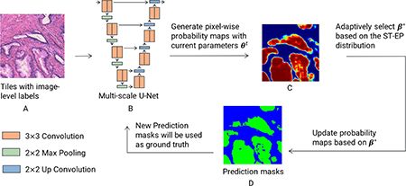
Fig. 4.

Overview of EM-based semi-supervised semantic segmentation. LMAs are generated by pathologists so that enclosed regions only contain tissues of the designated label (e.g. A ‘G3+3’ contour should contain purely G3 glands and stroma, devoid of benign glands or glands of other grades). EMbased algorithms are initialized with a multi-scale U-Net (as shown in B) trained on small amount of tiles with gland-level annotations, and trained on tiles with only image-level labels (as shown in A) extracted from LMAs on histopathological slides. In the E-step, the current model is applied to generate pixel-wise probability maps (as shown in C). To prevent the model from degeneracy, these probability maps are updated by a bias that has been adaptively selected by minimizing the KL divergence between the prior stroma versus epithelium distribution and the average model output distribution. Prediction masks (as shown in D) generated from the E-step are utilized to optimize model parameters in the Mstep. To improve training, a small portion of patches with gland-level annotations are combined with patches with image-level labels in each batch. The EM-based method will iteratively update segmentation masks and model parameters until convergence. (Figures are best viewed in color.)

4. Experiment

Here, we introduce the dataset utilized to develop and evaluate EM algorithms in Section 4.1. Then we show implementation and training details about the multi-scale U-Net model and EM methods in Section 4.2.

4.1. Dataset and image preprocessing

Our EM-based semi-supervised models were evaluated using a dataset obtained from the Department of Pathology at Cedars-Sinai Medical Center (IRB approval numbers: Pro00029960 and Pro00048462) that consists of data from three different cohorts (Gertych et al., 2015; Ing et al., 2018; Li et al., 2017):

1. 224 tiles with a size of 1200 × 1200, which contain stroma (ST), benign glands (BN), low-grade (G3) and high-grade areas (G4 with cribriform and non-cribriform glands) extracted from slides of prostatectomy specimens of 20 patients. These tiles were annotated at pixel-wise level by consensus of three uropathologists.

2. 289 tiles with a size of 1200 × 1200, which contain ST, BN, low-grade, and high-grade (G4 and G5) areas obtained from slides of 20 patients other than in set (A). These tiles were annotated in a similar manner as set (A) by or under direct supervision of an expert research pathologist.

3. A research pathologist provided LMAs on 30 whole slide images from prostatectomies of 30 patients by circling and grading the major foci of tumor as either low-grade (LG), high-grade (HG) or BN areas using the Aperio ScanScope software. Tiles extracted from the LMA were annotated with the same tilelevel label as the contour.

The scanning objective for all slides was set to 20× (0.5 𝜇𝑚 per pixel). Tiles were normalized using color transfer algorithm (Reinhard et al., 2001) to account for stain variability. 60% of the tiles from set (A) were used to train a multi-scale U-Net model and the remaining 40% were used to validate model hyperparameters. EM-based approaches initialized by that supervised model were trained to further improve semantic segmentation performance on around 1,800 weakly labeled tiles extracted from LMAs in set (C). Hyper-parameters were tuned on 89 left-out tiles from set (A) and model performances were evaluated on set (B) such that tiles from the same patient were not included in both training and testing.

4.2. Evaluation metric

Two commonly used metrics for semantic segmentation were employed for model evaluation: overall pixel accuracy (OP) and J. OP computes the proportion of correctly pixels, which can be easily biased by imbalanced datasets. J, also referred to as the intersection-over-union (IoU), can overcome the class imbalanced problem since it considers both false positives and negatives (Csurka et al., 2004; Everingham et al., 2015, 2010).

Both J and OP can be obtained from a pixel-wise confusion matrix C. C_ij is the number of pixels labeled as i and predicted as j. The total number of pixels with label i is denoted as $T_i={\sum }_{j=1}^N{C}_{i,j}$, where N is the number of classes. The number of pixels predicted as j is represented as P_j = ∑_iC_i,j (Csurka et al., 2004). The J for class i is then defined as follows (Li et al., 2017):

$$J_i=\frac{C_{i,i}}{T_i+P_i-C_{i,i}}$$

4.3. Details on model implementation and training

Given the large number of model parameters, we adopted two typically used regularization strategies: batch normalization (BN) and dropouts. The BN layer was applied after each convolutional layer except the final fully convolutional layer (Ioffe and Szegedy, 2015). Dropout layers with 0.5 probability were added in the deepest stage of the multi-scale U-Net (Ronneberger et al., 2015; Srivastava et al., 2014). The initial fully supervised multi-scale U-Net was trained on 135 tiles with batch stochastic gradient descent (batch size: 25). EM-based models were initialized with the multi-scale U-Net, and trained with stochastic gradient descent (batch size: 25) in M-steps. Hyper-parameters (e.g. learning rate, number of epochs, weight decay, etc.) were tuned on the validation set. The best result was obtained by using a momentum of 0.9, 0.0005 weight decay and a learning rate which was initialized as 0.005, reduced to and fixed at 0.001 after 5 epochs. For EM-fixed models, we used a 𝛽 value of 0.6 according to the average stroma-epithelium distribution across all classes. In EM-adaptive training, the optimal 𝛽 for each epithelial class was determined based on the prior distribution. For comparison, we implemented the adaptive method in (Papandreou et al., 2015).

Models were implemented in Torch 7 (Collobert et al., 2011) with two NVIDIA Titan X GPUs. Multiple separate data loading threads were used to accelerate training and testing. The average time required to generate a prediction mask for one 1,200 × 1,200 tile was around 9 seconds.

5. Results

Table 1 shows J and OP for models: EM adaptive model w/o fully annotated samples proposed in (Papandreou et al., 2015), EM-fixed w/o fully annotated samples (EM-fixed w/o), EM-fixed with 10% fully annotated samples (EM-fixed w 10%), etc. The initial multi-scale U-Net trained with 135 fully annotated tiles achieved a mean 𝐽 = 35.90% on an independent test set. EM-fixed and EM-adaptive models improved segmentation performance by incorporating information embedded in weakly labeled tiles extracted from LMAs of prostatectomy slides. Using an adaptive threshold resulted in significant improvements in J for low grade glands, high grade glands, and stroma (p<10⁻⁵_, p<10⁻²⁵, and p<10⁻¹⁸, respectively), and a nonsignificant decrease in J for benign glands (p=0.18). The average J and OP both significantly improved when using an adaptive threshold (p<10⁻¹⁸ and p<10⁻¹⁹, respectively). The baseline EM model w/o fully annotated samples (Papandreou et al., 2015) achieved mean 𝐽 = 42.32% and 𝑂𝑃 = 71.84%, which was significantly lower than the EM-adaptive w/o (p < 10⁻¹⁴ and p < 10⁻¹⁶, respectively).

Table 1.

Model performances on segmenting stroma, high-grade (HG), low-grade (LG), and benign (BN) glands.

	JLG (%)	JHG (%)	JBN (%)	JST (%)	Jmean (%)	OP (%)
Multi-scale U-Net	25.80	27.73	24.24	65.83	35.90	64.72
Papandreou et al. (2015)	30.80	50.13*	19.66	68.60	42.32	71.84
EM-fixed w/o	33.29	44.89*	23.11	67.26	42.14*	71.11*
EM-fixed w 10%	46.84	30.62	35.93	62.04	43.86*	67.28*
EM-fixed w 30%	43.59	28.17	35.11	61.76	42.16	66.62*
EM-fixed w 60%	41.82	26.43	30.59	61.23	40.02	65.27
EM-fixed w 90%	39.30	25.61	30.17	60.77	38.96	64.58
EM-adaptive w/o	33.20	52.01*	23.15	70.27*	44.66*	73.87*
EM-adaptive w 10%	49.67	42.08*	33.45	65.90*	47.78*	71.92*
EM-adaptive w 30%	48.25	49.58*	31.20	68.85*	49.47*	74.79*
EM-adaptive w 60%	46.36	42.17*	29.65	66.23*	46.10*	71.61*
EM-adaptive w 90%	40.07	35.62*	31.36	64.10	42.79*	68.65*

^*Denotes significant improvement over multi-scale U-Net using Wilcoxon signed-rank tests and Bonferroni correction for multiple comparisons.

To analyze the contribution of fully annotated samples, different percentages (10%, 30%, 60%, and 90%) of fully annotated patches were mixed with weakly labeled samples in each mini-batch during training. The performance of both EM-fixed and EM-adaptive models improved by adding a small portion of fully annotated samples. For example, the EM-adaptive model with 10% fully annotated samples achieved J_mean = 47.78%, which was about 3% higher compared to the EM-adaptive model without fully annotated samples. In addition, the EM-adaptive models consistently performed better than the EM-fixed models. The overall highest J_mean was obtained at 49.47% by the EM-adaptive model with 30% fully annotated samples. In Fig. 5, we show visual comparisons for semantic segmentation on some representative tiles from the test set.

Fig. 5.

Segmentation masks for tiles in the test set. The high-grade cancer (G4 or G5), low-grade cancer (G3), benign glands and stromal areas are indicated by red, pink, green, and blue colors respectively. The first column shows that the initial model delivers inferior performance in segmenting epithelial areas, likely due to the small amount of available supervised training data. Both EM-based models (shown in the second and third columns) are able to improve segmentation performance using weakly labeled tiles as they prevent the overestimation of stroma due to the optimization of beta. The best performance is achieved by combining 30% fully annotated tiles during EM training. (Figures are best viewed in color.)

6. Discussion

In this study, we demonstrated that EM-based algorithms can learn visual representations from histopathological slides with LMAs. A small portion of fully annotated samples increased J on low grade and benign epithelium, but reduced J on high grade and stroma areas, possibly because the limited fully annotated dataset did not contain all types of high grade tissues (G4 and G5). Moreover, adaptive biases based on prior knowledge of stroma-epithelium distribution lead to better EM training. We note that, realistically, our model’s performance remains insufficient for clinical deployment. Nonetheless, our novel methodology for incorporating weak supervision improves on the state of the art.

As shown in Table 1, the initial multi-scale U-Net model only achieved a mean J at 35.90%. The initial model failed to capture the HG glands and erroneously classified those areas into LG, or BN as shown in the first row of Fig. 5. Since we started with a training set with only 135 fully annotated tiles, the model may have been overfitted to this small dataset and did not generalize well to unseen samples. Furthermore, the HG class in our initial supervised training set only contained non-cribriform G4 and cribriform G4 growth patterns, but not G5 areas with hardly distinguishable glands. We would argue that the multi-scale U-Net may not have sufficient knowledge about visual representations of G5 areas.

Initialized with this undertrained model, our EM-based approaches were able to leverage rich information embedded in the large-scale weakly labeled dataset. Table 1 shows that all EM-based methods outperformed the initial model by a large margin. The mean J improved over 5% by most EM-based models, which demonstrates the ability of our semi-supervised algorithms in extracting useful signals from weakly labeled data. Both fixed and adaptive biases were imposed on pixel-wise probability maps to encourage pixels to be classified as the labeled class or stroma. This significantly reduced the possibility of misclassification of epithelium, such as predicting pixels in an LG tile as HG. As shown in the first and third rows of Fig. 5, the initial model predicted many HG areas as LG, BN or ST. However, the EM-adaptive model with 30% fully annotated samples correctly identified the approximate location of HG tissues, although it might be challenging to get perfect segmentation for HG areas, which have less recognizable glandular boundaries and may infiltrate into surrounding tissues. This kind of imprecise segmentation may be acceptable clinically, since localization of HG areas is considered to be more critical than accurate segmentation.

The baseline EM model (Papandreou et al., 2015) adaptively selected bias to constrain for each tile: at least ρ percentage of the tile to be predicted as foreground (epithelium). However, this method didn’t take account of differences of stroma-epithelium among individual classes (e.g., High-grade areas tend to have more epithelium). As shown in Table 1, the baseline EM model achieved a similar performance as the EMfixed model.

Different from the baseline EM model, the proposed bias was adaptively selected by minimizing the KL divergence between the model output distribution and the prior stroma-epithelium distribution. These models selected the optimal bias at the cost of longer training time since prediction maps had to be updated whenever a new bias was applied. We found that adding a small percent of strongly labeled data from the initial training set significantly improved model performance. However, adding too much strongly labeled data might prevent the model from learning new information from the large-scale weakly annotated dataset and lead to suboptimal performance. As seen in Table 1, the EM-adaptive model with 30% fully annotated samples achieved the highest mean J = 49.47% and OP = 74.79%.

There are several limitations in our work. First, we assume that each LMA contour contains one type of epithelium (BN, HG or LG), and tiles within the contour inherit its annotation as image-level labels. However, there still may be a very small portion of areas with different Gleason grades. In future work, we plan to extend our current EM-based approach to a multi-class weakly supervised model. Second, we only use a multi-scale U-Net proposed in our previous work as the backbone to generate segmentation masks. In future work, different state-of-the-art multi-scale architectures will also be explored and plugged into our semi-supervised training pipeline. In addition, cross-applicability is important for models that can be extended to computer aided diagnosis tools. We also plan to evaluate our approaches on whole slide images from different institutions, which may have distinct staining or scanning protocols.

7. Conclusion

In this paper, we proposed an EM-based semi-supervised model to leverage useful representations embedded in large-scale weakly annotated datasets. Adaptive biases incorporated prior knowledge on stroma versus epithelium distributions and were employed to prevent the model from predicting everything as stroma. The learning of the EM-based models was further improved by combining some fully annotated samples in each mini-batch during training. Our best semi-supervised EM-based approach achieved an average J of 49.47% on an independent test set, which was 14% higher than the supervised model. The result demonstrated that our semi-supervised model could improve semantic segmentation performance without requiring a very large dataset with time-consuming and costly pixel-wise annotations from pathologists.

Highlights.

• A semi-supervised model for histopathological image segmentation

• An EM-based framework to improve semantic segmentation with a large-scale weakly-labeled dataset

• Adaptive biases improve performance by incorporating prior knowledge during EM training

References

- Andrews S, Tsochantaridis I, Hofmann T, 2003. Support vector machines for multiple-instance learning, in: Advances in Neural Information Processing Systems. pp. 577–584. [Google Scholar]
- Arganda-Carreras I, Turaga SC, Berger DR, Cireşan D, Giusti A, Gambardella LM, Schmidhuber J, Laptev D, Dwivedi S, Buhmann JM, Liu T, Seyedhosseini M, Tasdizen T, Kamentsky L, Burget R, Uher V, Tan X, Sun C, Pham TD, Bas E, Uzunbas MG, Cardona A, Schindelin J, Seung HS, 2015. Crowdsourcing the creation of image segmentation algorithms for connectomics. Front. Neuroanat 9, 142. [DOI] [PMC free article] [PubMed] [Google Scholar]
- Badrinarayanan V, Kendall A, Cipolla R, 2015. SegNet: A Deep Convolutional Encoder-Decoder Architecture for Image Segmentation. [DOI] [PubMed]
- Bishop CM, 2006. Pattern recognition. Mach. Learn 128, 1–58. [Google Scholar]
- Chen H, Qi X, Yu L, Heng P-A, 2016. DCAN: Deep Contour-Aware Networks for Accurate Gland Segmentation, in: The IEEE Conference on Computer Vision and Pattern Recognition (CVPR) pp. 2487–2496. [Google Scholar]
- Chen L-C, Papandreou G, Kokkinos I, Murphy K, Yuille AL, 2017a. DeepLab: Semantic Image Segmentation with Deep Convolutional Nets, Atrous Convolution, and Fully Connected CRFs. IEEE Trans. Pattern Anal. Mach. Intell 1–1. 10.1109/TPAMI.2017.2699184 [DOI] [PubMed] [Google Scholar]
- Chen L-C, Papandreou G, Schroff F, Adam H, 2017b. Rethinking Atrous Convolution for Semantic Image Segmentation.
- Collobert R, Kavukcuoglu K, Farabet C, 2011. Torch7: A Matlab-like Environment for Machine Learning. BigLearn, NIPS Work. 1–6. [Google Scholar]
- Csurka G, Larlus D, Perronnin F, Meylan F, 2004. What is a good evaluation measure for semantic segmentation? IEEE PAMI. [Google Scholar]
- Dietterich TG, Lathrop RH, Lozano-Pérez T, 1997. Solving the multiple instance problem with axisparallel rectangles. Artif. Intell 89, 31–71. [Google Scholar]
- Doyle S, Feldman M, Tomaszewski J, Madabhushi A, Caicedo JJC, Lazebnik S, 2012. A Boosted Bayesian Multiresolution Classifier for Prostate Cancer Detection From Digitized Needle Biopsies. IEEE Trans. Biomed. Eng 59, 1205–1218. [DOI] [PubMed] [Google Scholar]
- Durand T, Thome N, Cord M, 2016. WELDON: Weakly Supervised Learning of Deep Convolutional Neural Networks, in: I EEE Conference on Computer Vision and Pattern Recognition (CVPR) pp. 4743–4752. [Google Scholar]
- Everingham M, Eslami SMA, Van Gool L, Williams CKI, Winn J, Zisserman A, 2015. The Pascal Visual Object Classes Challenge: A Retrospective. Int. J. Comput. Vis 111, 98–136. [Google Scholar]
- Everingham M, Van Gool L, Williams CKI, Winn J, Zisserman A, 2010. The Pascal Visual Object Classes (VOC) Challenge. Int. J. Comput. Vis 88, 303–338. [Google Scholar]
- Farjam R, Soltanian-Zadeh H, Jafari-Khouzani K, Zoroofi RA, 2007. An image analysis approach for automatic malignancy determination of prostate pathological images. Cytom. Part B Clin. Cytom 72B, 227–240. [DOI] [PubMed] [Google Scholar]
- Gertych A, Ing N, Ma Z, Fuchs TJ, Salman S, Mohanty S, Bhele S, Velásquez-Vacca A, Amin MB, Knudsen BS, 2015. Machine learning approaches to analyze histological images of tissues from radical prostatectomies. Comput. Med. Imaging Graph 46, 197–208. [DOI] [PMC free article] [PubMed] [Google Scholar]
- Gorelick L, Veksler O, Gaed M, Gomez JA, Moussa M, Bauman G, Fenster A, Ward AD, 2013. Prostate histopathology: Learning tissue component histograms for cancer detection and classification. IEEE Trans. 32, 1804–1818. [DOI] [PubMed] [Google Scholar]
- Gupta MR, Chen Y, 2010. Theory and Use of the EM Algorithm. Found. Trends Signal Process. 4, 223–296. [Google Scholar]
- Hamdy FC, Donovan JL, Lane JA, Mason M, Metcalfe C, Holding P, Davis M, Peters TJ, Turner EL, Martin RM, Oxley J, Robinson M, Staffurth J, Walsh E, Bollina P, Catto J, Doble A, Doherty A, Gillatt D, Kockelbergh R, Kynaston H, Paul A, Powell P, Prescott S, Rosario DJ, Rowe E, Neal DE, 2016. 10-Year Outcomes after Monitoring, Surgery, or Radiotherapy for Localized Prostate Cancer. N. Engl. J. Med 375, 1415–1424. [DOI] [PubMed] [Google Scholar]
- He K, Zhang X, Ren S, Sun J, 2016. Deep Residual Learning for Image Recognition, in: IEEE Conference on Computer Vision and Pattern Recognition pp. 770–778. [Google Scholar]
- Hou L, Samaras D, Kurc TM, Gao Y, Davis JE, Saltz JH, 2016. Patch-based Convolutional Neural Network for Whole Slide Tissue Image Classification. IEEE Comput. Soc. Conf. Comput. Vis. Pattern Recognit 2016, 2424–2433. [DOI] [PMC free article] [PubMed] [Google Scholar]
- Huang CC, Kong MX, Zhou M, Rosenkrantz AB, Taneja SS, Melamed J, Deng F-M, 2014. Gleason Score 3 + 4=7 Prostate Cancer With Minimal Quantity of Gleason Pattern 4 on Needle Biopsy Is Associated With Low-risk Tumor in Radical Prostatectomy Specimen. Am. J. Surg. Pathol 38, 1. [DOI] [PubMed] [Google Scholar]
- Humphrey PA, 2004. Gleason grading and prognostic factors in carcinoma of the prostate. Mod. Pathol 17, 292–306. [DOI] [PubMed] [Google Scholar]
- Ing N, Ma Z, Li J, Salemi H, Arnold CW, Knudsen BS, Gertych A, 2018. Semantic segmentation for prostate cancer grading by convolutional neural networks, in: SPIE Medical Imaging. Houston, Texas United States, pp. 10581–46. [Google Scholar]
- Ioffe S, Szegedy C, 2015. Batch Normalization: Accelerating Deep Network Training by Reducing Internal Covariate Shift, in: Proceedings of the 32nd International Conference on Machine Learning pp. 448–456. [Google Scholar]
- Jia Z, Huang X, Chang EI-C, Xu Y, 2017. Constrained Deep Weak Supervision for Histopathology Image Segmentation. IEEE Trans. Med. Imaging 36, 2376–2388. [DOI] [PubMed] [Google Scholar]
- Kraus OZ, Ba JL, Frey BJ, 2016. Classifying and segmenting microscopy images with deep multiple instance learning. Bioinformatics 32, i52–i59. [DOI] [PMC free article] [PubMed] [Google Scholar]
- Kwak JT, Hewitt SM, Kajdacsy-Balla AA, Sinha S, Bhargava R, 2016. Automated prostate tissue referencing for cancer detection and diagnosis. BMC Bioinformatics 17. [DOI] [PMC free article] [PubMed] [Google Scholar]
- Lavery HJ, Droller MJ, Michalski J, Al E, 2012. Do Gleason Patterns 3 and 4 Prostate Cancer Represent Separate Disease States? J. Urol 188, 1667–1675. [DOI] [PubMed] [Google Scholar]
- LeCun Y, Bengio Y, Hinton G, 2015. Deep learning. Nature 521, 436–444. [DOI] [PubMed] [Google Scholar]
- LeCun Y, Botos L, Benign Y, Haffner P, 1998. Gradient-based learning applied to document recognition, in: Proceedings of the IEEE. pp. 2278–2324. [Google Scholar]
- Li J, Sarma KV, Ho KC, Gertych A, Knudsen BS, Arnold CW, 2017. A Multi-scale U-Net for Semantic Segmentation of Histological Images from Radical Prostatectomies, in: AMIA Annual Symposium Proceedings. [PMC free article] [PubMed] [Google Scholar]
- Long J, Shelhamer E, Darrell T, 2015. Fully convolutional networks for semantic segmentation, in: IEEE Conference on Computer Vision and Pattern Recognition (CVPR) IEEE, pp. 3431–3440. [DOI] [PubMed] [Google Scholar]
- Maron O, Lozano-Pérez T, 1998. A framework for multiple-instance learning. Adv. neural Inf 570–576. [Google Scholar]
- Nguyen K, Sabata B, Jain AK, 2012a. Prostate cancer grading: Gland segmentation and structural features. Pattern Recognit. Lett 33, 951–961. [Google Scholar]
- Nguyen K, Sarkar A, Jain AK, 2012b. Structure and Context in Prostatic Gland Segmentation and Classification, in: International Conference on Medical Image Computing and Computer-Assisted Intervention Springer, Berlin, Heidelberg, pp. 115–123. [DOI] [PubMed] [Google Scholar]
- Papandreou G, Chen L-C, Murphy K, Yuille AL, 2015. Weakly-and Semi-Supervised Learning of a Deep Convolutional Network for Semantic Image Segmentation, in: IEEE International Conference on Computer Vision pp. 1742–1750. [Google Scholar]
- Peng Y, Jiang Y, Eisengart L, Healy MA, Straus FH, Yang XJ, 2011. Segmentation of prostatic glands in histology images, in: 2011 IEEE International Symposium on Biomedical Imaging: From Nano to Macro IEEE, pp. 2091–2094. [Google Scholar]
- Pinheiro PO, Collobert R, 2015. From Image-level to Pixel-level Labeling with Convolutional Networks, in: IEEE Conference on Computer Vision and Pattern Recognition pp. 1713–1721. [Google Scholar]
- Ramon J, De Raedt L, 2000. Multi Instance Neural Networks, in: ICML Workshop on Attribute-Value and Relational Learning pp. 53–60. [Google Scholar]
- Reinhard E, Adhikhmin M, Gooch B, Shirley P, 2001. Color transfer between images. IEEE Comput. Graph. Appl 21, 34–41. [Google Scholar]
- Ronneberger O, Fischer P, Brox T, 2015. U-Net: Convolutional Networks for Biomedical Image Segmentation. Med. Image Comput. Comput. Interv 9351, 234–241. [Google Scholar]
- Sermanet P, Eigen D, Zhang X, Mathieu M, Fergus R, LeCun Y, 2013. OverFeat: Integrated Recognition, Localization and Detection using Convolutional Networks.
- Siegel RL, Miller KD, Jemal A, 2016. Cancer statistics, 2016. CA. Cancer J. Clin 66, 7–30. [DOI] [PubMed] [Google Scholar]
- Simonyan K, Zisserman A, 2015. Very Deep Convolutional Networks for Large-Scale Image Recognition, in: International Conference on Learning Representations. [Google Scholar]
- Srivastava N, Hinton G, Krizhevsky A, Sutskever I, Salakhutdinov R, 2014. Dropout: A Simple Way to Prevent Neural Networks from Overfitting. J. Mach. Learn. Res 15, 1929–1958. [Google Scholar]
- Szegedy C, Wei Liu, Yangqing Jia, Sermanet P, Reed S, Anguelov D, Erhan D, Vanhoucke V, Rabinovich A, 2015. Going deeper with convolutions, in: IEEE Conference on Computer Vision and Pattern Recognition (CVPR) IEEE, pp. 1–9. [Google Scholar]
- Viola P, Platt JC, Zhang C, 2005. Multiple instance boosting for object detection. Proc. 18th Int. Conf. Neural Inf. Process. Syst [Google Scholar]
- Wang J, MacKenzie JJD, Ramachandran R, Chen DZ, 2016. A Deep Learning Approach for Semantic Segmentation in Histology Tissue Images, in: International Conference on Medical Image Computing and Computer-Assisted Intervention Springer, pp. 176–184. [Google Scholar]
- Wu J, Yinan Yu, Chang Huang, Kai Yu, 2015. Deep multiple instance learning for image classification and auto-annotation, in: 2015 IEEE Conference on Computer Vision and Pattern Recognition (CVPR) IEEE, pp. 3460–3469. [Google Scholar]
- Xu Y, Zhang J, Chang EI-C, Lai M, Tu Z, 2012a. Context-Constrained Multiple Instance Learning for Histopathology Image Segmentation, in: International Conference on Medical Image Computing and Computer-Assisted Intervention Springer, Berlin, Heidelberg, pp. 623–630. [DOI] [PubMed] [Google Scholar]
- Xu Y, Zhu J-Y, Chang E, Tu Z, 2012b. Multiple clustered instance learning for histopathology cancer image classification, segmentation and clustering, in: 2012 IEEE Conference on Computer Vision and Pattern Recognition IEEE, pp. 964–971. [Google Scholar]
- Xu Y, Zhu J-Y, Chang EI-C, Lai M, Tu Z, 2014. Weakly supervised histopathology cancer image segmentation and classification. Med. Image Anal 18, 591–604. [DOI] [PubMed] [Google Scholar]
- Zhang C, Platt J, Viola P, 2005. Multiple instance boosting for object detection. Adv. neural. [Google Scholar]