A Visually Interpretable, Dictionary-Based Approach to Imaging-Genomic Modeling, With Low-Grade Glioma as a Case Study

Abstract

Radiomics is a rapidly growing field in which sophisticated imaging features are extracted from radiology images to predict clinical outcomes/responses, genetic alterations, and other outcomes relevant to a patient’s prognosis or response to therapy. This approach can effectively capture intratumor phenotypic heterogeneity by interrogating the “larger” image field, which is not possible with traditional biopsy procedures that interrogate specific subregions alone. Most models in radiomics derive numerous imaging features (eg, texture, shape, size) from a radiology data set and then learn complex nonlinear hypotheses to solve a given prediction task. This presents the challenge of visual interpretability of radiomic features necessary for effective adoption of radiomic models into the clinical decision-making process. To this end, we employed a dictionary learning approach to derive visually interpretable imaging features relevant to genetic alterations in low-grade gliomas. This model can identify regions of a medical image that potentially influence the prediction process. Using a publicly available data set of magnetic resonance imaging images from patients diagnosed with low-grade gliomas, we demonstrated that the dictionary-based model performs well in predicting 2 biomarkers of interest (1p/19q codeletion and IDH1 mutation). Furthermore, the visual regions (atoms) associated with these dictionaries show association with key molecular pathways implicated in gliomagenesis. Our results show that dictionary learning is a promising approach to obtain insights into the diagnostic process and to potentially aid radiologists in selecting physiologically relevant biopsy locations.

Introduction

Medical diagnosis using radiology images has become increasingly common in the past century. Recent advances in image processing and computer vision have allowed the extraction of diverse high-dimensional measurements from images in the form of imaging features, leading to increased interest in the fields of Radiomics and Radiogenomics. In Radiomics, imaging features are extracted from medical images and used to predict outcomes such as tumor grade and overall survival.^1–3 Radiogenomics, also called “imaging-genomics,” aims to study relationships between extracted imaging features and genomic alterations.^4,5

In a conventional clinical scenario, a doctor must biopsy the patient’s tumor to assess characteristics such as malignancy, grade, and underlying genetic mutations to make treatment decisions. This process has 3 primary limitations:

1. Invasiveness: An invasive procedure is expensive and is confounded by the availability of viable tissue surrounding the biopsy location,⁶ in addition to presenting certain associated comorbidities.

2. Temporal variability: Rarely are multiple biopsy samples obtained longitudinally over time, thus direct observation of tumor growth trajectory is often infeasible.

3. Incomplete consideration of intratumor heterogeneity: A biopsy is obtained from only one part of the tumor and therefore cannot account for intratumor heterogeneity. Recent studies have shown that biopsies taken at different locations in a tumor result in different gene expression profiles.⁷ This highlights the importance of biopsy locations and the potentially faulty diagnoses that result from improper and inadequate sampling.

However, medical imaging is a noninvasive diagnostic modality that can be performed repeatedly over time with the potential to capture intratumor heterogeneity, circumventing the above issues. Radiomic and Radiogenomic techniques capable of predicting tumor characteristics usually assessed via biopsy have the potential to replace the biopsy routine entirely or at least serve as viable surrogates where such directed sampling is infeasible or contraindicated.

Present approaches in Radiomics and Radiogenomics are based primarily on morphologic (shape, volume, size) and textural analysis.^1,4,^8,9 Typically, a large number of texture features are extracted, and various feature selection methods are employed to reduce their dimensionality. Various classification models such as support vector machine (SVMs), neural networks, and random forests are then trained on these features. This approach has produced powerful predictive models but suffers from notable disadvantages:

1. Texture features are calculated over the entire tumor region and therefore fail to preserve voxel-level intensity variations. These descriptors typically provide a single summary value that does not adequately capture the spatial gray-level heterogeneity within the entire tumor. In a multicompartmental tumor setting that includes distinct subregions such as edema, necrosis, enhancing, and nonenhancing regions; such a characterization neglects the variation between these biologically distinct regions.

2. Although these models may demonstrate excellent predictive accuracy, they employ learning algorithms that output predictions with confidence intervals (CIs), but no interpretable information (eg, no insight into which visual features are specifically being used to arrive at a decision). This lack of interpretability is a major obstacle in the automation of tumor diagnosis. If a clinician’s biopsy and a model’s prediction disagree, then despite the model’s proven predictive accuracy, it will be infeasible for health care professionals to trust the model and arrive at an appropriate diagnosis.

To provide insight into the visual features influencing outcome prediction, our proposed approach analyzes voxel subregions (“patches”) across the tumor region of a magnetic resonance imaging (MRI) image and extracts feature descriptors only from those patches. Such an approach captures tumor spatial heterogeneity by analyzing multiple such subregions across the tumor area. A dictionary-based method to identify data-driven representations of these sampled patches is then used to build a predictive model for relevant outcomes (genomic characteristics, survival, etc). Such dictionary elements are much more interpretable in the context of a predictive model because they are directly visualizable, thus providing insight into specific characteristics of tumor subregions related to clinical outcome. Furthermore, such information could direct neurosurgeons and neuroradiologists to specific regions of the tumor that are most informative for biopsy and subsequent molecular characterization and outcome modeling.

Materials and Methods

Data set

This study was conducted using a set of 108 low-grade glioma (LGG) patient cases from The Cancer Genome Atlas imaging data collection with linked preoperative MRI imaging, clinical, and genomic data. The MRI images from 4 distinct sequences are available: fluid-attenuated inversion recovery (FLAIR), T1-weighted (T1w) precontrast, T2-weighted (T2w), and T1-weighted postcontrast (T1c). T1-weighted postcontrast images were excluded from analysis because LGGs do not display any significant enhancement characteristics in T1-postcontrast imaging. Few patients had only a subset of these MRI sequences. This resulted in a data set with 86 FLAIR images, 102 T1w precontrast images, and 105 T2-weighted images. The neoplasm histologic grade of patients is either grade 2 or grade 3. Of the 108 unique patients in the study, 52 have grade 2 tumors and 56 have grade 3 tumors. The tumor histology is astrocytoma, oligodendroglioma, or oligoastrocytoma. Of the 108 unique patients in the study, 31 have astrocytoma, 29 have oligodendroglioma, and 48 have oligoastrocytoma. This histologic data can be found in the clinical data files of patients. The acquisition protocols are also varied which makes the data highly heterogeneous.

The outcomes of interest to our study were 2 molecular biomarkers with prognostic value¹⁰ for individual patient outcome: (1) the mutation status of IDH1 gene and (2) the presence of codeletion of chromosome arms 1p and 19q. The IDH1 biomarker is determined by whether the gene is mutated or wild type, and this biomarker is of particular interest because it has been shown that patients with mutated IDH1 tend to have longer survival than patients with wild-type IDH1.¹¹ Similarly, patients with chromosomal 1p/19q codeletion have been shown to generally have better prognoses than patients lacking the codeletion; in particular, patients with the codeletion respond better to radiochemotherapy.¹¹ As both of these categorical variables are binary, the corresponding classification tasks are both two-class. Furthermore, of the 108 patients in the data set, 85 had IDH1 mutation, and 26 had 1p/19q codeletion; thus, both classification tasks were notably unbalanced.

Preprocessing

Three-dimensional (3D) tumor volumes were segmented within each MRI scan by experienced radiologists (H.B., C.S.). Because imaging was performed at multiple institutions, the natural variation in imaging acquisition protocols, equipment, etc, requires that the imaging data be intensity-standardized prior to analysis—this permits comparison of imaging intensities across multiple MRI scans across all patients in the data set. To this end, we employed white stripe normalization—a white matter intensity–based normalization technique implemented in the R computing language. The white stripe normalization algorithm is designed for neuroimaging data and has been shown to outperform histogram-based methods for voxel intensity normalization on brain MRI images.¹²

Imaging features

Each tumor volume from an MRI scan is a 3D array of voxel intensities, which was transformed for input into a classifier (after feature extraction). Our analysis compared predictive performance of 3 common approaches for generating feature variables from the (intensity normalized) tumor volume. Each approach relies on sampling of square “patches” of voxels from consecutive 2-dimensional horizontal slices comprising the given 3D tumor volume. On the basis of literature review and empirical experimentation, we decided to sample 140 patches, each 16 × 16 voxels, per patient.¹³ The first of the 3 imaging descriptor approaches simply uses voxel intensities from the patch as input to the classifier in the form of a 256-dimensional column vector. The second approach uses the histogram of oriented gradients (HOG) descriptor. Here, a feature vector is extracted by decomposing the patch into a grid of smaller squares, each of size 4 × 4; calculating a HOG in each square; and concatenating those histograms.¹⁴ The third approach uses the scale-invariant feature transform (SIFT) descriptor. Here, feature vectors are generated by detecting local extrema in the voxel intensities and calculating oriented histograms only at these extrema.¹⁴ Both HOG and SIFT features have been used commonly in image classification tasks.^15,16

Classification of genetic alteration status

This study compared 2 machine learning models (Bag of Words [BoW] and dictionary learning approach with structured incoherence [DLSI], more details below) that can provide spatial interpretability for the MRI images. Identifying regions within the tumor volume that influence predictive performance can assist clinicians obtain insight into the physiologic basis of patient’s diagnosis. A more detailed discussion of interpretability is provided in the “Results” section.

Bag of Words

The baseline predictive model, the BoW-based learning algorithm, is routinely employed in computer vision tasks where visual interpretability is essential. It combines the BoW approach^17,18 with k-means centroid clustering and an SVM. As noted in section “Imaging features,” this approach relies on the sampling of voxel patches. Feature extraction, the process of transforming the patches into numerical representations accessible to a learning model, is done by either vectorizing the patch voxel intensities or computing the HOG/SIFT descriptors. This approach then performs k-means clustering over the set of these computed descriptor vectors. The cluster centroids constitute the “words” in the codebook. For each patient in the training set, a histogram of “word counts” is computed across the sampled patches by assigning each patch to the centroid that approximates it most closely. These histograms can then be used as feature vectors for training machine learning models such as SVM and neural networks to predict genetic alteration status.

Compared with k-means clustering, k-median clustering uses 1-norm distance to update the centroids rather than 2-norm. This property makes k-median more reliable and suitable for discrete or binary data sets. However, as the update rule is based on a 1-norm minimization problem, k-median is relatively slow. In our problem, in particular, and computer vision applications, in general, descriptors are usually continuous, and then k-means is more suitable. In fact, most of well-known BoW-related feature extractors in the literature use k-means clustering.^17,19

Dictionary learning (with DLSI)

The proposed dictionary-based model employs the DLSI, an algorithm introduced by Ramirez et al.²⁰ The algorithm is motivated by sparse coding,^21,22 in which a given signal is approximated as a sparse linear combination of a few basis elements. These basis elements are individually referred to as “atoms” and collectively referred to as a “dictionary.” Just as the BoW model learns a codebook of “visual words” from the data through clustering, the dictionary-based model learns a data-driven dictionary through sparse regression. The primary difference between the BoW and dictionary learning models is that while the BoW model clusters an input to the single nearest word in the codebook, the dictionary learning model uses a combination of multiple atoms in approximating the input signal to better discriminate between voxel patches. In addition, the DLSI model learns a discriminative dictionary, one for each outcome class—rather than learning a single codebook as in the BoW.

Experimental procedures

We evaluated BoW/DLSI approaches for various feature descriptors (HOG, raw voxel intensities, and SIFT descriptors) across various MRI sequences. The best-performing DLSI model in terms of area under the receiver operating characteristic curve (AUC)²³ employs the hyperparameters η = 1 and λ = 0.1.²⁴ Stratified 10-fold crossvalidation repeated 5 times over the data set was used for iterative model training and validation, resulting in 50 AUC estimates for each model. Stratified k-fold crossvalidation methods prevent overfitting on unbalanced data sets. The final AUC estimate presented for a given model is the mean of these 50 AUCs, whereas the corresponding 95% CI was obtained through 2000 bootstrap iterations over these 50 AUCs. P values comparing the AUC values between 2 models were calculated through a Mann-Whitney test. “All experiments are performed in MATLAB and the relevant programs are provided on GitHub [github.com/wdeaderick/Radiomics_DictLearn].”

Results

Classification

For prediction of IDH1 mutation, the strongest-performing model was the DLSI model trained on raw voxel intensity descriptors extracted from T2-weighted images. This approach obtained a mean AUC of 0.8224 (CI: 0.7856-0.8575). For 1p/19q codeletion prediction task, the strongest performing model was again the DLSI model trained on raw voxel intensity descriptors from T1w precontrast images. This model obtained a mean AUC of 0.6854 (CI: 0.6291-0.7379).

Figure 1 compares IDH1 mutation prediction results between the dictionary-based (DLSI) models against BoW models trained with each of the 3 descriptors. This figure considers only models trained on the T2-weighted images, as these imaging sequences proved to be the most predictive of IDH1 mutation. Similarly, Figure 2 compares 1p/19q codeletion prediction results between the dictionary-based models and BoW models trained on each of the 3 descriptors. This figure considers only the models trained on T1w precontrast images, as this imaging sequence was found to be the most predictive of 1p/19q codeletion.

Figure 1.

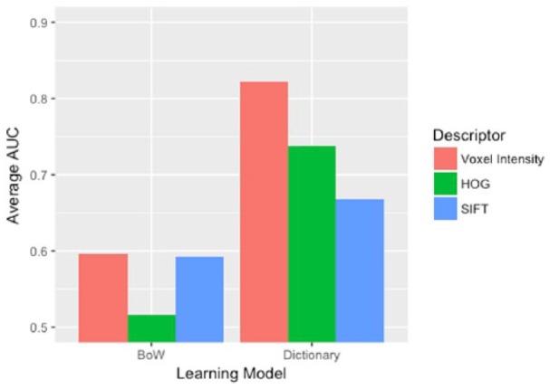
Prediction of IDH1 mutation based on T2-weighted MRI sequence. IDH1 mutation prediction results of dictionary-based (DLSI) models and BoW models trained with each of the 3 descriptors. In this figure, only results from T2-weighted images are presented as this imaging sequence is most predictive of IDH1 mutation. AUC indicates area under the receiver operating characteristic curve; BoW, Bag of Words; DLSI, dictionary learning approach with structured incoherence; HOG, histogram of oriented gradients; SIFT, scale-invariant feature transform.

Figure 2.

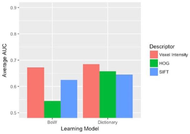
T1-sequence–based prediction of 1p/19q codeletion status. 1p/19q codeletion prediction results of dictionary-based models and BoW models trained on each of the 3 descriptors. In this figure, only results from T1w precontrast images are presented as this imaging sequence is most predictive of 1p/19q codeletion. AUC indicates area under the receiver operating characteristic curve; BoW, Bag of Words; HOG, histogram of oriented gradients; SIFT, scale-invariant feature transform; T1w, TI weighted.

As is clear from Figures 1 and 2, across learning algorithms and classification tasks, using vectorized voxel intensities as the descriptor outperformed the usage of either the HOG descriptor or the SIFT descriptor. Although HOG and SIFT descriptors have been applied with great success in a variety of image classification scenarios, the abstraction offered by these descriptors failed to provide any additional discriminative information in the context of patch-based IDH1 and 1p/19q prediction.

The dictionary-based model also consistently outperformed the BoW model. Table 1 presents the mean AUCs (and corresponding CIs) for both the dictionary-based model and the BoW model (trained on vectorized voxel intensities from the T1w precontrast images, for both classification tasks). Tables 2 and 3 present corresponding results from the T2-weighted and FLAIR sequence, respectively. At a significance level of α = .05, the dictionary-based model had a significantly higher mean AUC than the corresponding BoW model for every imaging sequence when predicting IDH1 mutation. The dictionary-based model again outperformed the BoW model when predicting 1p/19q codeletion on 2 of the 3 imaging sequences.

Table 1.

Comparison of models trained on voxel intensities from T1-weighted precontrast magnetic resonance imaging data.

Classification	Dictionary model	Bow model	P value
IDH1 mutation, AUC (95% CI)	0.73 (0.68-0.77)	0.44 (0.37-0.49)	2.6 × 10−10
1p/19q codeletion, AUC (95% CI)	0.69 (0.63-0.74)	0.67 (0.61-0.72)	.73

Abbreviations: AUC, area under the receiver operating characteristic curve; BoW, Bag of Words; CI, confidence interval.

Table 2.

Comparison of models trained on voxel intensities from T2-weighted magnetic resonance imaging data.

Classification	Dictionary model	Bow model	P value
IDH1 mutation, AUC (95% CI)	0.82 (0.79-0.86)	0.60 (0.53-0.67)	4.7 × 10−7
1p/19q codeletion, AUC (95% CI)	0.63 (0.57-0.69)	0.59 (0.53-0.65)	.36

Abbreviations: AUC, area under the receiver operating characteristic curve; BoW, Bag of Words; CI, confidence interval.

Table 3.

Comparison of models trained on voxel intensities from fluid-attenuated inversion recovery sequence data.

	Dictionary model	Bow model	P value
IDH1 mutation, AUC (95% CI)	0.63 (0.58-0.69)	0.46 (0.39-0.54)	6.3 × 10−4
1p/19q codeletion, AUC (95% CI)	0.55 (0.47-0.62)	0.56 (0.48-0.64)	.82

Abbreviations: AUC, area under the receiver operating characteristic curve; BoW, Bag of Words; CI, confidence interval.

Interpretability

In addition to predicting the genomic status of IDH1 or 1p/19q, the dictionary-based model could also identify the tumor subregions that most influenced predictive performance. This information is displayed in the form of a heatmap, overlaid on the tumor region of interest and referred to as a “Patch Importance” (PI) plot. Areas of the PI plot with higher intensity values indicate regions of the tumor that strongly influence the algorithm’s prediction. It is reasonable to assume that these regions are more likely to be biologically relevant to the genomic trait of interest. To mitigate the noise associated with scores across the spatial extent of the tumor, we employed Gaussian smoothing. A PI plot generation procedure is shown in Figure 3. The PI plots containing predominantly low values would be seen only in extreme cases where the randomly sampled patches on which the model based its overall prediction were notably unrepresentative of the tumor as a whole.

Figure 3.

Patch Importance (PI) plot generation procedure. (A) fluid-attenuated inversion recovery magnetic resonance image of tumor region. (B) Patchwise prediction (the orange triangles in this image are the patchwise prediction locations that correspond to the boxes in first figure). (C) Smoothed PI plot using Gaussian smoothing. Dark orange regions are more important than blue regions in making predictions.

The PI plot corresponding to a patient with IDH1 mutation is shown in Figure 4. As this PI plot is very largely high scoring, we can infer that the model was quite confident in its prediction for this case, across the entire tumor region of interest.

Figure 4.

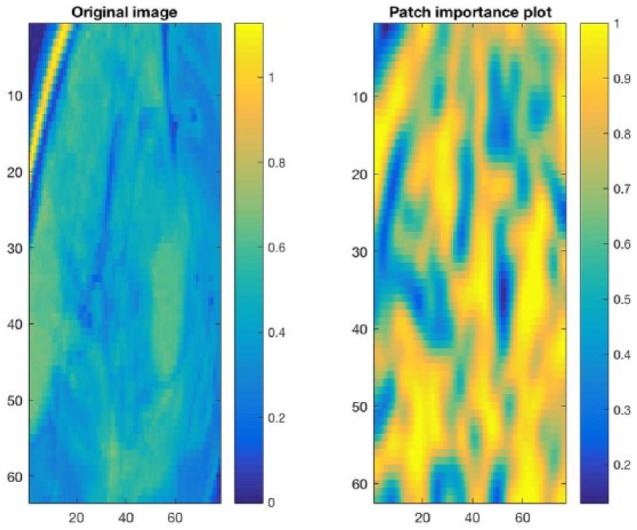
Patch Importance (PI) plot for correctly predicted IDH1 mutation. This PI plot corresponds to a patient with IDH1 mutation. As this PI plot is largely high scoring, we can infer that the model was quite confident in its prediction, across the entire tumor region of interest.

Correlation with molecular pathways

In addition to the PI plots, we observed that the molecular pathways of the patients were associated with the DLSI-derived dictionary atoms. Figure 5 shows the Pearson correlation between molecular pathways and dictionary representation in the context of IDH1 prediction. Benjamini-Hochberg procedure was used to correct for multiple hypothesis testing, and pathways most significantly correlated with the dictionary atoms were selected. A false discovery rate or q value cutoff of .25 was used to assess significance. This analysis resulted in 57 molecular pathways that were strongly associated with at least 1 dictionary atom. The clustergram of this correlation matrix is shown in Figure 5. Dictionary atoms are found to be associated with multiple molecular pathways associated with gliomagenesis such as PTK2, AKT1, and FOXO,^25,26 lending biological relevance to the derived dictionary atoms.

Figure 5.

Clustergram of correlation matrix. A total of 57 molecular pathways (vertical axis) are correlated with 218 dictionary atoms. This clustergram shows the set of pathways that play a role in IDH1 gene mutation. Dictionary atoms contain pathway information and are therefore useful to make accurate gene mutation predictions.

Discussion

For both classification tasks, the DLSI dictionary-based model consistently outperformed the BoW model, and vectorized voxel intensity descriptors yielded better performance than HOG and SIFT descriptors. Therefore, dictionary learning models give promising prediction accuracies as well as provide visual interpretability through PI plots.

Dictionary learning with structured incoherence algorithm employed in our model is a simple approach to dictionary learning. In recent years, approaches using a shared-class dictionary to account for traits common to multiple classes, as well as approaches imposing constraints that promote discriminative information in the sparse coding coefficients themselves, have been introduced.^27,28 As dictionary learning algorithms continue to improve and become increasingly capable of identifying the subtle yet discriminative differences between signals of opposing classes, we can expect both the classification efficacy and the biological interpretability of our learning framework to improve in the long term.

In addition, although there exist many imaging descriptors beyond HOG and SIFT, it is surprising that the strongest performing descriptors are voxel intensities of the normalized MRI images. The PI plots generated by the dictionary-based model can be used in radiologic, neuropathologic, and neurosurgical settings to aid health care professionals choose more informative locations for biopsy. Typically, a pathologist will choose a location for biopsy based on distance from the skull, as regions closer to the skull are presumed to be safer for such invasive procedures. Such a sampling method is not particularly well informed and may result in inaccurate or incomplete diagnosis owing to incorrect sampling and ignoring intratumor heterogeneity. Therefore, PI plots could provide additional insight in choosing a biopsy location. The PI plots also provide information regarding a tumor’s heterogeneity; as the variation in tumor histologic characteristics and concomitant heterogeneity becomes better appreciated clinically, the utility of such PI plots would potentially increase as well.

Both dictionary learning and BoW algorithms could predict IDH1 mutation status better than the remaining genomic information. This is probably because IDH1 mutation is shown to have oncogenic effects that can be identifiable from MRI scans.^29,30 The authors in Molenaar et al²⁹ argue that prolonged survival of IDH1-mutated patients is possibly from slower tumor growth due to distributed cellular metabolism. This causes changes in histologic and radiologic features such as lower edema, necrosis, and larger nonenhancing tumor regions, all of which can potentially be detected using Radiomics.

A discussion of a potential limitation of the PI plot is also in order. The final algorithm does not have 100% accuracy, so the overall prediction made on a patient’s clinical outcome may be incorrect sometimes. The PI plot uses this prediction to assign positive or negative color to the patches. The PI plot will be inverted if the overall prediction is incorrect. Also, MRI data from only 108 patients are used to build the machine learning algorithms. Obtaining more training data and capturing the full spectrum of patient-associated heterogeneity will result in improved accuracies, less data bias, and possibly better resolution in the PI plots.

Conclusions and Future Work

We have shown that dictionary learning–based approaches provide visually interpretable feature information accompanying these predictive models. They could potentially aid radiologists to select relevant biopsy locations informed through PI plots. Therefore, this methodology has the potential to aid a collaborative relationship between the radiologist and a computer-based decision support system interrogating tumor heterogeneity.

Exploration of other advanced dictionary learning algorithms would further validate the performance and feasibility of this approach. Also, the predictive results reported here are based on each single MRI sequence type used individually. With proper image registration methods, one can combine information from different sequences and build a model that uses the multiparametric information synergistically. We anticipate that fusing multiple MRI sequences might further improve predictive performance.

References

- 1. Lambin P, Rios-Velazquez E, Leijenaar R, et al. Radiomics: extracting more information from medical images using advanced feature analysis. Eur J Cancer. 2012;48:441–446. [DOI] [PMC free article] [PubMed] [Google Scholar]
- 2. Gillies RJ, Kinahan PE, Hricak H. Radiomics: images are more than pictures, they are data. Radiology. 2015;278:563–577. [DOI] [PMC free article] [PubMed] [Google Scholar]
- 3. Vallieres M, Freeman CR, Skamene SR, El Naqa I. A radiomics model from joint FDG-PET and MRI texture features for the prediction of lung metastases in soft-tissue sarcomas of the extremities. Phys Med Biol. 2015;60:5471–5496. [DOI] [PubMed] [Google Scholar]
- 4. Aerts HJ, Velazquez ER, Leijenaar RT, et al. Decoding tumour phenotype by noninvasive imaging using a quantitative radiomics approach. Nat Commun. 2014;5:4006. [DOI] [PMC free article] [PubMed] [Google Scholar]
- 5. Segal E, Sirlin CB, Ooi C, et al. Decoding global gene expression programs in liver cancer by noninvasive imaging. Nat Biotechnol. 2007;25:675–680. [DOI] [PubMed] [Google Scholar]
- 6. National Institute of Health. The Cancer Genome Atlas (TCGA) database. http://cancergenome.nih.gov. Accessed April 17, 2017.
- 7. Gerlinger M, Rowan AJ, Horswell S, et al. Intratumor heterogeneity and branched evolution revealed by multiregion sequencing. N Engl J Med. 2012;366:883–892. [DOI] [PMC free article] [PubMed] [Google Scholar]
- 8. Zhou H, Vallières M, Bai HX, et al. MRI features predict survival and molecular markers in diffuse lower-grade gliomas. Neuro Oncol. 2017;19:862–870. [DOI] [PMC free article] [PubMed] [Google Scholar]
- 9. Parmar C, Grossmann P, Bussink J, Lambin P, Aerts HJ. Machine learning methods for quantitative radiomic biomarkers. Sci Rep. 2015;5:13087. [DOI] [PMC free article] [PubMed] [Google Scholar]
- 10. Ceccarelli M, Barthel FP, Malta TM, et al. Molecular profiling reveals biologically discrete subsets and pathways of progression in diffuse glioma. Cell. 2016;164:550–563. [DOI] [PMC free article] [PubMed] [Google Scholar]
- 11. Brat DJ, Verhaak RG, Aldape KD, et al. Comprehensive, integrative genomic analysis of diffuse lower-grade gliomas. N Engl J Med. 2015;372:2481–2498. [DOI] [PMC free article] [PubMed] [Google Scholar]
- 12. Shinohara RT, Sweeney EM, Goldsmith J, et al. Statistical normalization techniques for magnetic resonance imaging. Neuroimage Clin. 2014;6:9–19. [DOI] [PMC free article] [PubMed] [Google Scholar]
- 13. Tong T. Patch-Based Image Analysis: Application to Segmentation and Disease Classification [dissertation]. London: Imperial College London; 2014. [Google Scholar]
- 14. Vedaldi A, Fulkerson B. VLFeat: an open and portable library of computer vision algorithms. http://www.vlfeat.org. Updated 2008. Accessed June 6, 2017.
- 15. Dalal N, Triggs B. Histograms of oriented gradients for human detection. Paper presented at: IEEE Computer Society Conference on Computer Vision and Pattern Recognition; June 20-25, 2005; San Diego, CA. [Google Scholar]
- 16. Lowe DG. Distinctive image features from scale-invariant keypoints. Int J Comput Vision. 2004;60:91–110. [Google Scholar]
- 17. Csurka G, Dance CR, Fan L, Willamowski J, Bray C. Visual categorization with bags of keypoints. Paper presented at: Workshop on Statistical Learning in Computer Vision (ECCV); May 11-14, 2004; Prague. [Google Scholar]
- 18. Fei-Fei L, Perona P. A Bayesian hierarchical model for learning natural scene categories. Paper presented at: IEEE Computer Society Conference on Computer Vision and Pattern Recognition; June 20-25, 2005; San Diego, CA. doi: 10.1109/CVPR.2005.16. [DOI] [Google Scholar]
- 19. Lazebnik S, Schmid C, Ponce J. Beyond bags of features: spatial pyramid matching for recognizing natural scene categories. Paper presented at: IEEE Computer Society Conference on Computer Vision and Pattern Recognition; June 17-22, 2006; New York, NY. [Google Scholar]
- 20. Ramirez I, Sprechmann P, Sapiro G. Classification and clustering via dictionary learning with structured incoherence and shared features. Paper presented at: IEEE Computer Society Conference on Computer Vision and Pattern Recognition; June 13-18, 2010; San Francisco, CA:3501–3508. doi: 10.1109/CVPR.2010.5539964. [DOI] [Google Scholar]
- 21. Tosic I, Pascal F. Dictionary learning. IEEE Signal Proc Mag. 2011;28:27–38. [DOI] [PubMed] [Google Scholar]
- 22. Xu Y, Li Z, Yang J, Zhang D. A survey of dictionary learning algorithms for face recognition. IEEE Access. 2017;5:8502–8514. doi: 10.1109/ACCESS.2017.2695239. [DOI] [Google Scholar]
- 23. Bradley AP. The use of the area under the ROC curve in the evaluation of machine learning algorithms. Pattern Recogn 1997;30:1145–1159. [Google Scholar]
- 24. Yang M, Zhang L, Feng X, Zhang D. Fisher discrimination dictionary learning for sparse representation. Paper presented at: IEEE International Conference on Computer Vision (ICCV); November 6-13, 2011; Barcelona. [Google Scholar]
- 25. Dunn GP, Rinne ML, Wykosky J, et al. Emerging insights into the molecular and cellular basis of glioblastoma. Genes Dev. 2012;26:756–784. [DOI] [PMC free article] [PubMed] [Google Scholar]
- 26. Kumar A, Rajendran V, Sethumadhavan R, Purohit R. AKT kinase pathway: a leading target in cancer research. Sci World J. 2013;2013:756134. [DOI] [PMC free article] [PubMed] [Google Scholar]
- 27. Vu TH, Monga V. Learning a low-rank shared dictionary for object classification. Paper presented at: International Conference on Image Processing; September 25-28, 2016; Phoenix, AZ. [Google Scholar]
- 28. Ubaru S, Seghouane AK, Saad Y. Improving the incoherence of a learned dictionary via rank shrinkage. Neural Comput. 2017;29:263–285. doi: 10.1162/NECOa00907. [DOI] [PubMed] [Google Scholar]
- 29. Molenaar RJ, Radivoyevitch T, Maciejewski JP, van Noorden CJ, Bleeker FE. The driver and passenger effects of isocitrate dehydrogenase 1 and 2 mutations in oncogenesis and survival prolongation. Biochim Biophys Acta. 2014;1846:326–341. [DOI] [PubMed] [Google Scholar]
- 30. Molenaar RJ, Verbaan D, Lamba S, et al. The combination of IDH1 mutations and MGMT methylation status predicts survival in glioblastoma better than either IDH1 or MGMT alone. Neuro Oncol. 2014;16:1263–1273. [DOI] [PMC free article] [PubMed] [Google Scholar]