Performance of intraclass correlation coefficient (ICC) as a reliability index under various distributions in scale reliability studies

Abstract

Many published scale validation studies determine inter‐rater reliability using the intra‐class correlation coefficient (ICC). However, the use of this statistic must consider its advantages, limitations, and applicability. This paper evaluates how interaction of subject distribution, sample size, and levels of rater disagreement affects ICC and provides an approach for obtaining relevant ICC estimates under suboptimal conditions. Simulation results suggest that for a fixed number of subjects, ICC from the convex distribution is smaller than ICC for the uniform distribution, which in turn is smaller than ICC for the concave distribution. The variance component estimates also show that the dissimilarity of ICC among distributions is attributed to the study design (ie, distribution of subjects) component of subject variability and not the scale quality component of rater error variability. The dependency of ICC on the distribution of subjects makes it difficult to compare results across reliability studies. Hence, it is proposed that reliability studies should be designed using a uniform distribution of subjects because of the standardization it provides for representing objective disagreement. In the absence of uniform distribution, a sampling method is proposed to reduce the non‐uniformity. In addition, as expected, high levels of disagreement result in low ICC, and when the type of distribution is fixed, any increase in the number of subjects beyond a moderately large specification such as n = 80 does not have a major impact on ICC.

1. INTRODUCTION

Central to the quality and usefulness of any research undertaking is the reliability of its data. Reliability, defined as the consistency of measurements, can be assessed by the intra‐class correlation coefficient (ICC).1 This index has been used in many fields to assess the quality of measurement tools from which conclusions of a study are drawn for FDA product approvals.2 In such settings, an experimental paradigm (eg, an assay) aims to establish the properties of the measurement tools under standardized conditions. Unlike clinical trials where the study population is not controlled, reliability studies allow for modifications to assess properties of the measurement tool under a more standardized setup. From a regulatory perspective, it is essential to produce reliable methods or tools that can be applied to different scales and enable comparison across them.

This paper addresses statistical issues for the reliability of measurement tools called “scales” as objective instruments for determining baseline severity and post‐treatment outcomes to evaluate treatment effectiveness. These scales are based on a Likert‐type design, consisting of phrases with or without photographs that define each category, commonly called grades. Scales that are a combination of phrases and photographs are known as photonumeric scales. In aesthetic studies, some examples of scales are measures for the degree of wrinkling,3, 4, 5, 6, 7, 8 lip fullness,9, 10, 11, 12 sagging,13 photodamage,14 and dyspigmentation,15 and they have been developed and evaluated using reliability indexes. In many aesthetic scale reliability studies, ICC is used to determine consistency, where a higher ICC signifies better consistency.3, 4, 5, 6, 7, 8, 9, 10, 11, 12, 13, 14, 16

In scale reliability studies, literature indicates that the distribution of subjects has an impact on ICC,17, 18, 19, 20, 21, 22 although there is no guidance regarding the number of subjects in each grade of the scale. Specifically, assessments of scales using subjects that are homogeneous tend to have poorer ICC than those that utilize more heterogeneous distributions of subjects. Thus, it may be critical to evaluate reliability of a scale with an equal distribution of subjects in each grade, which creates a more standardized setting.23 This, however, may be difficult to achieve under certain circumstances. For instance, when multiple scales are evaluated simultaneously, there is minimal control on the distribution of subjects in each scale. Also, when the scales being evaluated involve traits for which the extreme grades are uncommon, enrolling equal number of subjects for all grades may be challenging. With the absence of uniformity in the distribution of subjects and the sensitivity of ICC to the composition of subjects in the respective grades, it is important to produce a more standardized environment as well as understand how any departure from such a standard affects the reliability measure.

The example used for illustration in this paper is a multiple scales reliability study designed to validate 5 photonumeric scales for measuring volume deficits and aging in the following areas: forehead lines, fine lines, hand volume deficit, skin roughness, and temple hollowing.24, 25, 26, 27, 28 Each of the 5 scales has 5 grades of severity (ie, 0 = none, 1 = slight, 2 = mild, 3 = moderate, 4 = severe) to measure volume deficit and aging. Because multiple scales are being assessed simultaneously, it is difficult to obtain uniform distributions of subjects across all 5 grades of the 5 scales as is apparent in Table 1. The mean rating of each subject across multiple raters is used to assess the distribution of the subjects across the 5 grades of the 5 scales.

Table 1.

Distribution of subjects enrolled in the study (N = 313) of the 5 photonumeric scales

Severity scale	P0	P1	P2	P3	P4	Total a	ICC
Fine lines	13.5%	38.4%	27.0%	13.1%	8.0%	289	0.61
Forehead lines	2.4%	27.1%	28.8%	24.4%	17.3%	295	0.82
Hand volume deficit	2.4%	28.4%	43.2%	22.3%	3.7%	296	0.73
Skin roughness	7.3%	39.3%	37.2%	10.7%	5.5%	290	0.68
Temple hollowing	4.4%	29.5%	36.9%	24.8%	4.4%	298	0.68

Note: P₀, P₁, P₂, P₃, and P₄ refer to the percentages of subjects having mean subject scores of 0, 1, 2, 3, and 4, respectively, across multiple raters.

^aNot all enrolled subjects qualified for all 5 scales as per the study inclusion‐exclusion criteria; hence, there are fewer than 313 subjects in the total column.

Inter‐rater reliability for this study was measured using ICC, which is a function of subject and rater error variance, where a lower rater error variance implies a reliable scale. As shown in Table 1, the ICC varied from 0.61 to 0.82 for the 5 scales. The comparability of ICC to a version of weighted kappa,29 for which a threshold is available for interpretation,30 enables an ICC of at least 0.6 to represent substantial reliability. Additional discussion of this example is provided in Section 5, where it is noted that the rater error variance is relatively small for all of the scales, and so the variation of ICC among the scales is due to the sensitivity of the ICC to the composition of subjects in the respective grades.

In view of this sensitivity, the calculated ICC could downgrade the reliability of the scale relative to the threshold.31 Accordingly, simulation studies are explored in this paper to shed additional light on such considerations and to enhance understanding of the impact of properties of distribution (eg, different distributions of subjects, sample size) on reliability indexes and their corresponding variance components. Also, methods are provided for adjusting the ICC to minimize the manner in which homogeneity of the population can downgrade reliability relative to the threshold.30

In this paper, ICC is the focus due to its flexibility as a reliability index. In this regard, it can be used as a measure for inter‐rater reliability (reliability between raters) and intra‐rater reliability (reliability within raters). Additionally, its formulation can be adapted to evaluate continuous or discrete scales as well as assessment of multiple raters. Lastly, among the available reliability indexes for continuous grades, ICC directly measures agreement in comparison to its counterparts, such as correlation coefficient r and linear regression, which measure association and not agreement.32 In this paper, the behavior of ICC is investigated under uniform and non‐uniform (convex, concave, and skewed) distributions (see Figure 1). This allows a quantitative comparison of ICC across distributions with varying degrees of homogeneity. Furthermore, the effect of sample size along with different levels of disagreement on the ICC estimate is examined.

Figure 1.

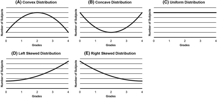
Types of distribution. A, The convex distribution has the least number of subjects in the extreme grades and the majority in the middle grade. B, The concave distribution has the least number of subjects in the middle grade and the majority in the extremes. C, The uniform distribution has subjects equally distributed across grades. D, The left skewed distribution has the majority of subjects in the extreme higher grades and the least number subjects in the extreme lower grades. E, The right skewed distribution has the majority of subjects in the extreme lower grades and the least number of subjects in the higher grades

The objective of this paper is to evaluate how the combination of subject distribution, sample size, and levels of disagreement affects ICC, and to provide an approach for obtaining ICC estimates under suboptimal conditions. This is particularly important in reliability studies of scales with low prevalence in some grades or in multiple scale reliability studies where simultaneous evaluation of several scales on the same subject are performed, making it difficult to control the heterogeneity of subjects for all scales. Hence, there is an inherent issue of dependency on population distributions that needs to be addressed in most of the scales being studied. It is also the goal of this paper to present a way of generating a more standardized structure to eliminate downgrading of agreement induced by homogeneity in the population.

Section 2 reviews ICC as a measure of reliability. Section 3 discusses the simulation setup and results that aid in understanding the behavior of ICC under different conditions, and it is followed by Section 4, which presents the proposed sampling method to provide more relevant and less distribution‐dependent ICC estimates and their corresponding simulation results. Section 5 shows the results of the motivating multiple scales reliability study and the application of the sampling method to reduce the impact of suboptimal conditions on ICC. Summarizing remarks are presented in Section 6.

2. INTRACLASS CORRELATION COEFFICIENT

The ICC is commonly used to evaluate the reliability of a scale with continuous or ordered categorical grades for n subjects with ratings by k raters. In many aesthetic scale reliability studies in the literature, the expected reliability of a single rater's grade is of interest, and the results from the study usually need to be generalized to a larger population of raters, with each subject being rated by every rater. Thus, the assumed study design corresponds to a set of k raters, randomly selected from a population, judging each of n randomly selected subjects. In such a case, the 2‐way ANOVA model has the specification in.1

$$X_{\mathit{ij}}=\mathrm{\mu }+a_i+b_j+{\left(\mathit{ab}\right)}_{\mathit{ij}}+{\in }_{\mathit{ij}}$$ (1)

where i = 1, 2, …, n subjects and j = 1, 2, …, k raters. In 1, X_{i  j} is the observed grade, a_i is the difference between μ and the i ^th subject's so‐called true grade, b_j is the difference between μ and the mean of the j ^th rater's grade, (ab)_{i  j} is the degree to which the j ^th rater differs from usual scoring tendencies when rating the i ^th subject, and ϵ_ij is the random error in the j ^th rater's grade for the i ^th subject. It is assumed that μ is a fixed overall population mean of the ratings, and the remaining model components are random with $a_i\sim N\left(0,{\sigma }_a^2\right),$ $b_j\sim N\left(0,{\sigma }_b^2\right),$ ${\left(\mathit{ab}\right)}_{\mathit{ij}}\sim N\left(0,{\sigma }_{\mathit{ab}}^2\right)$, and ${ϵ}_{\mathit{ij}}\sim N\left(0,{\sigma }_{ϵ}^2\right)$. Hence, $X_{\mathit{ij}}\sim N\left(\mu ,{\sigma }_a^2+{\sigma }_b^2+{\sigma }_{\mathit{ab}}^2+{\sigma }_{ϵ}^2\right)$ and $\mathit{Cov}\left(X_{\mathit{ij}},X_{i{j}^{\prime }}\right)={\sigma }_a^2$. Under this scenario, the parameter of interest is the agreement index ρ or the inter‐rater ICC, which is a ratio of $\left\{\frac{\mathit{Cov}\left(X_{\mathit{ij}},X_{i{j}^{\prime }}\right)}{\mathit{Var}\left(X_{\mathit{ij}}\right)}\right\}$ as shown in.2

$$\rho =\frac{{\sigma }_a^2}{{\sigma }_a^2+{\sigma }_b^2+{\sigma }_{\mathit{ab}}^2+{\sigma }_{\in }^2}$$ (2)

For estimation of ρ, the variance components can be estimated as ${\widehat{\sigma }}_a^2=\frac{\mathit{BMS}-\mathit{EMS}}{k},$ ${\widehat{\sigma }}_b^2=\frac{\mathit{JMS}-\mathit{EMS}}{n}$, and ${\widehat{\sigma }}_{\mathit{ab}}^2+{\widehat{\sigma }}_{ϵ}^2=\mathit{EMS}$. Thus, the estimator $\widehat{\rho }$ can be derived as.3

$$\widehat{\rho }=\frac{{\widehat{\sigma }}_a^2}{{\widehat{\sigma }}_a^2+{\widehat{\sigma }}_b^2+{\widehat{\sigma }}_{\mathit{ab}}^2+{\widehat{\sigma }}_{ϵ}^2}=\frac{\mathit{BMS}-\mathit{EMS}}{\mathit{BMS}+\left(k-1\right)\mathit{EMS}+\frac{k}{n}\left(\mathit{JMS}-\mathit{EMS}\right)}$$ (3)

where (a) BMS is the between‐subjects mean square in 4 and refers to the departure of the mean grade across repeated ratings on the i^th subject from the overall mean; (b) JMS is the between‐raters mean square in 5 and refers to the departure of the mean across repeated ratings of the j^th rater from the overall mean; and (c) EMS is the residual mean square in 6 and refers to the departure of the j^th rater from their usual ratings on the i^th subject.

$$\mathit{BMS}=\frac{k{\sum }_{i=1}^n{\left({\overline{x}}_{i.}-{\overline{x}}_{..}\right)}^2}{n-1}$$ (4)

$$\mathit{JMS}=\frac{n{\sum }_{j=1}^k{\left({\overline{x}}_{.j}-{\overline{x}}_{..}\right)}^2}{k-1}$$ (5)

$$\mathit{EMS}=\frac{{\sum }_{i=1}^n{\sum }_{j=1}^k{\left(x_{\mathit{ij}}-{\overline{x}}_{i.}-{\overline{x}}_{.j}+{\overline{x}}_{..}\right)}^2}{\left(n-1\right)\left(k-1\right)}$$ (6)

While the previously noted estimates are based on a normal distribution, this assumption is not necessary for the valid estimation of ICC. Thus, such estimation of ICC is applicable for uniform and non‐uniform distributions as illustrated in Figure 1.

It is important that the behaviors of these variance components (ie, ${\widehat{\sigma }}_a^2,{\widehat{\sigma }}_b^2$ and ( ${\widehat{\sigma }}_{\mathit{ab}}^2+{\widehat{\sigma }}_{ϵ}^2$)) are understood in relation to ICC. Based on the above formulation, it can be seen that ${\widehat{\sigma }}_a^2$ assesses only subject variability and is absent of any scale or rater quality information; thus, ${\widehat{\sigma }}_a^2$ focuses on the study design component. Meanwhile, ${\widehat{\sigma }}_b^2+{\widehat{\sigma }}_{\mathit{ab}}^2+{\widehat{\sigma }}_{ϵ}^2$ measures rater error variability, where smaller values imply more reliable scales. Hence, the reliability of the scale as assessed by ICC can also be evaluated by the rater error variance estimate ${\widehat{\sigma }}_b^2+{\widehat{\sigma }}_{\mathit{ab}}^2+{\widehat{\sigma }}_{ϵ}^2$. However, low rater error variability does not guarantee a high ICC because a low subject variance, ${\widehat{\sigma }}_a^2$, will still produce a low ICC. This effect of subject variance on ICC indicates the need to minimize the impact of study design on ICC. Based on its formula in, 2 it is theoretically difficult to assess the degree to which the distribution of subjects has an impact on ICC. Thus, we evaluate the behavior of ICC through simulation studies, using uniform and non‐uniform distributions to depict different levels of heterogeneity. The behavior of the variance components is likewise investigated.

It is acknowledged that there are other available measures used to evaluate scale quality through the information on the variance components. One such metric is called the within‐subject coefficient of variation (WCV) which considers the ratio of $\sqrt{{\sigma }_b+{\sigma }_{\mathit{ab}}+{\sigma }_{ϵ}}$ and μ to determine the reliability of scales.33 While this alternative measure can be used for comparing scales applied on varying population distributions, WCV may be sensitive to subject distributions with different means. In such cases, it would be challenging to compare the reliability across different studies or scales. Furthermore, unlike ICC, WCV does not have an available threshold for determining the reliability of a scale, making its interpretation difficult. This also presents some difficulties in creating a standardized criterion for the acceptance of scales and setting conditions for assessment of scales.

Another reasonable measure of reliability is the concordance correlation coefficient (CCC), which characterizes the agreement of 2 variables by the expected value of the squared differences.34 The CCC has been further extended to measure overall agreement among multiple raters, as well as evaluated to establish its equivalence to ICC under valid ANOVA assumptions.35 It has been shown that under fixed ${\sigma }_b^2+{\sigma }_{\mathit{ab}}^2+{\sigma }_{ϵ}^2$, both ICC and CCC increase as ${\sigma }_a^2$ increases; hence, like ICC, subject distribution also has on an impact on the CCC.31 However, the formulation of CCC for 2 raters34 as well as its extension for multiple raters36 suggest that the observed grades are from fixed raters. Because it is of more interest to look into the impact of raters as a random effect, ICC is considered for investigation rather than CCC. Moreover, ICC is often used in the regulatory environment, particularly for aesthetic scales. Hence, ICC is the focus of the paper.

3. IMPACT OF DISTRIBUTION, SAMPLE SIZE, AND DISAGREEMENTS ON ICC

One of the objectives of this paper is to assess the impact of properties of distribution and levels of disagreement on ICC. To that end, data sets were simulated to mimic real‐life scenarios of scale reliability studies by controlling the following factors:

• Sample size

• Distribution of subjects in each grade

• Levels of disagreement across grades

The effect of having a large versus a small number of subjects is investigated to illustrate the importance of sample size. If ICC estimates obtained using a smaller sample size are similar to those obtained from a larger sample, then study costs may be reduced without sacrificing the quality of the generated ICC, although it is recognized that sample size needs to be large enough to produce sufficiently accurate ICC for assessment. Moreover, some scale reliability studies are only able to recruit relatively few subjects in less common grades, leading to a less heterogeneous distribution of subjects. Thus, by examining different levels of disagreement, the simulation study evaluates the effect of rater and scale quality on ICC. Results based on these factors may influence the design of the reliability study as well as guidelines for rater recruitment and training, and so the simulations explore the behavior of ICC for different combinations of the above 3 factors.

3.1. Simulation setup

In each of the 10 000 simulations performed, k = 8 raters assessed N subjects on a 5‐point ordinal scale ranging from 0 to 4. For every subject i = 1, 2, …N judged by a specific rater j = 1, 2, …, k, a discrete, observed grade X_{i  j} is simulated. The observed grade X_{i  j} is simulated by defining a master grade, which represents a subject's true grade and some level of measurement error or disagreement from the true grade. If there is no disagreement, the observed grade will be equal to the defined master grade. Otherwise, the observed grade will be a sum of the defined master grade and some degree of disagreement. In real‐life reliability studies, the true or master grade would be the gold standard. However, many reliability studies in aesthetics often do not have a gold standard and no master grade exists. In such cases, the subject grade at recruitment can be used as the master grade to assess the distribution of subjects for the scale grades.

A total of N = 300 and N = 80 subjects were simulated to illustrate the effect of sample size on ICC. The choice of N = 300 is considered because it provides a large number of subjects. Meanwhile, the use of N = 80 provides a sufficient sample size because ICC estimates based on N = 80 are similar to those from N = 300, as will be shown in Section 3.2.

With respect to the distribution of subjects, scenarios reflected in Figure 1 , namely concave, convex, uniform, and skewed distributions, were investigated. This is an essential point of inquiry in the simulation setup, as it pertains to the effect of various types of populations on ICC. When each master grade has the same number of subjects, as in the case of the uniform distribution, the population is said to have completely balanced heterogeneity. Conversely, a higher number of subjects in a specific master grade compared with the remaining grades leads to a more non‐uniform population. This is realized for concave, convex, and skewed distributions. More specifically, convex distributions have a large number of subjects concentrated in the middle grades and the number of subjects decreases substantially for the extreme grades. Conversely, in concave distributions, the middle grades have fewer subjects, and the number of subjects increases toward the extreme grades. However, the degree of departure from the uniform distribution may vary from 1 distribution to another. For instance, 1 convex distribution may have more subjects in the extreme grades compared with another convex distribution; thus, the former is a mild convex distribution while the latter is an extreme convex distribution. The same disparity in the degree of imbalance may be exhibited among concave distributions. Skewed distributions have other forms of imbalance, for which a large number of subjects are concentrated towards 1 extreme of the scale and taper off towards the other extreme. These cases of imbalance were considered in the simulation setup, and although results for the skewed distributions are not shown, conclusions regarding their effect on ICC are presented.

Data sets of sample sizes $N={\sum }_{g=0}^4{N}_g=300$ and N = 80, where N_g = number of subjects having master grade g = 0, 1, 2, 3, 4, were simulated by generating samples from the fixed aforementioned distributions of master grades described in Table 2 and randomly invoking disagreements as prescribed in Table 3. In the simulation setup, the number of subjects chosen from each grade is fixed. This suggests that there is no random component involved when defining the population structure of the subjects.

Table 2.

Distribution of master grades with N = 300 and N = 80

Distribution Type	Distribution of Subjects per Grade (%)	Sample Size	N0	N1	N2	N3	N4
Extreme concave	P0 = 33.0%, P1 = 16.7 % , P2 = 4.0%, P3 = 14.0%, P4 = 32.3%	N = 300	99	50	12	42	97
		N = 80	27	13	3	11	26
Mild concave	P0 = 29.7%, P1 = 16.7 % , P2 = 7.3%, P3 = 15.3%, P4 = 31.0%	N = 300	89	50	22	46	93
		N = 80	24	13	6	12	25
Uniform	P0 = 20%, P1 = 20 % , P2 = 20%, P3 = 20%, P4 = 20%	N = 300	60	60	60	60	60
		N = 80	16	16	16	16	16
Mild convex	P0 = 6.7%, P1 = 24.0 % , P2 = 36.0%, P3 = 27.0%, P4 = 6.3%	N = 300	20	72	108	81	19
		N = 80	5	19	29	22	5
Extreme convex	P0 = 2.3%, P1 = 28.7 % , P2 = 42.7%, P3 = 22.7%, P4 = 3.6%	N = 300	7	86	128	68	11
		N = 80	2	23	34	18	3

Note: P₀, P₁, P₂, P₃, and P₄ refer to the percentages of subjects having master grades 0, 1, 2, 3, and 4, respectively.

Table 3.

Cases pertaining to different levels of disagreement

Case Number	Nature of Disagreement
1	• 20% subjects with 1‐point disagreement for all raters (k = 8)
2	• 20% subjects with 1‐point disagreement for 75% of the raters (k = 6)
	• 30% subjects with 1‐point and 20% subjects with 2‐point disagreement for 25% of the raters (k = 2)
3	• 20% subjects with 1‐point disagreement for 50% of the raters (k = 4)
	• 30% subjects with 1‐point and 20% subjects with 2‐point disagreement for 50% of the raters (k=4)
4	• 20% subjects with 1‐point disagreement for 25% of the raters (k = 2)
	• 30% subjects with 1‐point and 20% subjects with 2‐point disagreement for 75% of the raters (k=6)
5	• 20% subjects with 1‐point disagreement, 10% subjects with 2‐point disagreement, 5%subjects with 3‐point disagreement and 5% subjects with 4‐point difference for 50% of the raters (k = 4)
	• 10% subjects with 1‐point disagreement, 10% subjects with 2‐point disagreement, 10%subjects with 3‐point disagreement, and 10% subjects with 4‐point difference for 50% of the raters (k = 4)
6	• 30% subjects with 1‐point disagreement, 10% subjects with 2‐point disagreement, 10%subjects with 3‐point disagreement, and 10% subjects with 4‐point difference for 50% of the raters (k = 4)
	• 20% subjects with 1‐point disagreement, 20% subjects with 2‐point disagreement, 10%subjects with 3‐point disagreement, and 10% subjects with 4‐point difference for 50% of the raters (k = 4)

For the levels of disagreement from the master grade, each rater was assigned a level of error in judgment, depicted by the grade differences, for a certain percentage of the subjects being rated. For instance, a rater who is said to have a 20% disagreement by a 1‐point difference is unable to properly judge the master grade for 20% of the subjects. This error is represented by a 1‐point difference between the observed grade and the master grade. Subjects whose grades differ from the master grade are selected randomly for each rater and need not be the same subject for every rater. Also, the movement of the grade differences is random; that is, a 1‐point difference given a master grade of 1 can be randomly represented by 0 or 2. However, for grades 0 and 4, a 1‐point difference implies a grade of 1 and 3, respectively, with a probability of 1. Additionally, these movements in grade differences are symmetric; thus, for a 4‐point difference, a master grade of 0 having an observed score of 4 and a master grade of 4 having an observed score of 0 are equally likely. Meanwhile, master grades 1, 2, or 3 have zero chance of observing a 4‐point difference. With the random and symmetric nature of the disagreements in this simulation setup, the contribution of b_j in 1 is minimal because ${\sigma }_b^2$ is expected to be almost null. Hence, in these simulations, the reliability of the scale is assessed by the rater error variance estimate as mainly determined by the quantity ${\widehat{\sigma }}_{\mathit{ab}}^2+{\widehat{\sigma }}_{ϵ}^2$ with very little contribution from ${\widehat{\sigma }}_b^2$.

In general, differences from the master grade represent rater and scale quality. Ideally, these disagreements from the master grade would be low. High disagreements imply that the scale is unable to properly capture the true measurement and differentiate the grades or that the raters are poorly trained in the use of the scale. Table 3 shows the different levels of disagreement for k = 8 raters considered in the simulation scenarios. Cases 1 through 6 depict varying extents of rater disagreement ranging from acceptable to extreme disagreement. It should be noted that for each of the 10 000 simulations, a random invocation of disagreements, as presented in Table 3, is performed on a set of subjects generated from a fixed distribution of master scores as shown in Table 2.

The observed scores for subject i by rater j are then calculated as the sum of the master grade and the level of disagreement defined for rater j as shown in Table 3. Therefore, the observed grades will not have the same distribution as the master grade. Scenarios with lower levels of disagreement, however, will produce less disparity between the distribution of subjects based on master grade and observed grade when compared with those with extreme disagreements.

It should be noted that although the simulated data were based on a master grade, this value was not included in ICC calculation.

The quantitative differences in ICC estimates and its variance components, as presented in Section 3.2, across different levels of disagreement, distributions, and sample size will describe the level of dependency of ICC on these factors. These results are presented in the following section.

3.2. Simulation results

The results of the 10 000 simulations illustrate the effect of external factors on ICC. Table 4 shows that holding the distribution constant, the total number of subjects used, N, has a negligible impact on ICC estimates. For instance, ICC values for N = 300 and N = 80 are similar for the extreme concave distribution in all 6 cases. This also holds true for uniform, mild concave, mild and extreme convex, and skewed distributions, with the differences ranging from 0.00 to 0.01 across all 6 cases. This offers an advantage in terms of cost and ease in data collection and management. However, the interdecile ranges suggest that as the number of subjects decreases, more variability in the estimates is realized particularly for higher levels of disagreement. It is also noted that the simulations were carried out for N = 70 and the same behavior was observed. Also, as expected, the ICC estimates decrease as the levels of disagreement from the master score increase, producing lower scale reliability.

Table 4.

Mean ICC (and interdecile range) across 10 000 simulations for uniform, convex, and concave distributions with large (N = 300) and small (N = 80) sample size

Distribution Type	Total Number of Subjects Enrolled	Levels of Disagreement
		Case 1	Case 2	Case 3	Case 4	Case 5	Case 6
Extreme concavea	N = 300	0.93 (0.01)	0.85 (0.02)	0.77 (0.02)	0.69 (0.02)	0.39 (0.05)	0.19 (0.04)
	N = 80	0.93 (0.01)	0.85 (0.03)	0.78 (0.04)	0.70 (0.05)	0.40 (0.10)	0.20 (0.09)
Mild concaveb	N = 300	0.93 (0.01)	0.84 (0.02)	0.76 (0.02)	0.68 (0.03)	0.38 (0.05)	0.19 (0.04)
	N = 80	0.93 (0.01)	0.84 (0.03)	0.76 (0.04)	0.68 (0.05)	0.39 (0.10)	0.20 (0.09)
Uniformc	N = 300	0.90 (0.01)	0.79 (0.02)	0.68 (0.03)	0.58 (0.03)	0.34 (0.05)	0.16 (0.04)
	N = 80	0.90 (0.02)	0.79 (0.04)	0.68 (0.06)	0.58 (0.06)	0.35 (0.10)	0.17 (0.09)
Mild convexd	N = 300	0.82 (0.02)	0.65 (0.03)	0.51 (0.04)	0.39 (0.04)	0.26 (0.06)	0.11 (0.04)
	N = 80	0.82 (0.03)	0.65 (0.06)	0.50 (0.07)	0.38 (0.08)	0.26 (0.10)	0.10 (0.08)
Extreme convexe	N = 300	0.78 (0.02)	0.58 (0.04)	0.43 (0.04)	0.30 (0.04)	0.22 (0.06)	0.08 (0.04)
	N = 80	0.78 (0.04)	0.58 (0.07)	0.43 (0.08)	0.31 (0.08)	0.23 (0.11)	0.09 (0.08)

^aExtreme concave distribution indicates having 33%, 16.7%, 4%, 14%, and 32.3% of the subjects in grades 0, 1, 2, 3, and 4, respectively.

^bMild concave distribution indicates having 29.7%, 16.7%, 7.3%, 15.3%, and 31.0% of the subjects in grades 0, 1, 2, 3, and 4, respectively.

^cUniform distribution indicates having 20% of the subjects in grades 0, 1, 2, 3, and 4.

^dMild convex distribution indicates having 6.7%, 24%, 36%, 27%, and 6.3% of the subjects in grades 0, 1, 2, 3, and 4, respectively.

^eExtreme convex distribution indicates having 2.3%, 28.7%, 42.7%, 22.7%, and 3.6% of the subjects in grades 0, 1, 2, 3, and 4, respectively.

Table 4 illustrates that for a fixed N, the uniform distribution provides higher ICC for all cases of disagreement when compared with extreme and mild convex distribution, with the difference ranging from 0.08 to 0.28 and 0.05 to 0.20, respectively. Similar relationships were observed between uniform and skewed distributions. However, this relation is reversed for concave distributions. ICC for extreme and mild concave distributions are higher than that for the uniform distribution, with the difference ranging from 0.03 to 0.12 and 0.03 to 0.10, respectively. Furthermore, the results also suggest that as the degree of non‐uniformity decreases, the ICC values tend to move towards the ICC under the uniform distribution.

This dependency of ICC on the subject distribution substantially changes the interpretation of ICC (ie, the quality of the scale being assessed) between the distributions, holding the other 2 factors constant. For example, in Case 2, the results suggest that based on the threshold,30 the strength of agreement among raters is almost perfect for the extreme concave distribution, substantial for the uniform distribution, and moderate for the extreme convex distribution.

Higher ICC estimates in the concave cases, where the extremes are represented more, may be due to a combination of 2 factors. First, the observed grades of subjects under concave distributions intuitively have larger differences from the mean which leads to a larger ${\widehat{\sigma }}_a^2.$Also, any deviation of the observed grades from the master grade results in a movement towards the middle grades. Specifically, the measurement error is reduced because a 1‐point or 2‐point difference in the extreme grades implies movement only in 1 direction (ie, towards the middle).

By contrast, lower ICC estimates in the convex case are calculated because the observed grades have smaller differences from the mean. Also, with more subjects in the middle grades, convex distributions have higher impact of measurement error because a 1‐point or 2‐point difference in the middle grades can move in 2 directions.

To further investigate reliability of a scale, the variance components of ICC were estimated for all of the scenarios presented above. As shown in Table 5, the subject variance estimates follow a behavior similar to ICC. In particular, highest ${\widehat{\sigma }}_a^2$ are obtained for concave distributions while ${\widehat{\sigma }}_a^2$ are lowest for convex distributions. Also, as the distribution of subjects across grades approaches the uniform distribution, so does the ${\widehat{\sigma }}_a^2.$ Given a fixed distribution, varying sample size produces approximately equal ${\widehat{\sigma }}_a^2$ that decreases as the levels of disagreement increase. Similarly, based on interdecile ranges, it can be established that while the ${\widehat{\sigma }}_a^2$ estimates are approximately the same, more stable estimates are realized when a larger number of subjects is used. Because ${\widehat{\sigma }}_a^2$ decreases from Case 1 to Case 6, it appears that the homogeneity of the observed distribution is increased as the levels of disagreements become severe. This consequently leads to lower ICC as shown in Table 4 .

Table 5.

Mean subject variance estimates, ${\widehat{\sigma }}_a^2$, (and interdecile range) across 10 000 simulations for uniform, convex, and concave distributions with large (N = 300) and small (N = 80) sample size

Distribution Type	Total Number of Subjects Enrolled	Levels of Disagreement
		Case 1	Case 2	Case 3	Case 4	Case 5	Case 6
Extreme concavea	N = 300	2.43 (0.06)	2.08 (0.08)	1.76 (0.09)	1.47 (0.09)	0.91 (0.13)	0.39 (0.09)
	N = 80	2.47 (0.12)	2.12 (0.16)	1.79 (0.18)	1.50 (0.19)	0.94 (0.25)	0.42 (0.19)
Mild concaveb	N = 300	2.29 (0.06)	1.96 (0.08)	1.65 (0.09)	1.38 (0.09)	0.86 (0.12)	0.37 (0.09)
	N = 80	2.32 (0.12)	1.99 (0.16)	1.68 (0.18)	1.40 (0.19)	0.89 (0.25)	0.39 (0.19)
Uniformc	N = 300	1.70 (0.05)	1.44 (0.07)	1.21 (0.08)	1.00 (0.08)	0.63 (0.10)	0.27 (0.08)
	N = 80	1.71 (0.11)	1.46 (0.14)	1.22 (0.16)	1.01 (0.16)	0.65 (0.21)	0.29 (0.16)
Mild convexd	N = 300	0.93 (0.04)	0.77 (0.05)	0.63 (0.06)	0.50 (0.07)	0.33 (0.08)	0.15 (0.06)
	N = 80	0.92 (0.07)	0.77 (0.10)	0.62 (0.11)	0.50 (0.12)	0.33 (0.13)	0.15 (0.11)
Extreme convexe	N = 300	0.70 (0.04)	0.58 (0.05)	0.47 (0.05)	0.36 (0.06)	0.24 (0.06)	0.11 (0.05)
	N = 80	0.72 (0.06)	0.59 (0.09)	0.47 (0.11)	0.37 (0.11)	0.25 (0.12)	0.12 (0.10)

^aExtreme concave distribution indicates having 33%, 16.7%, 4%, 14%, and 32.3% of the subjects in grades 0, 1, 2, 3, and 4, respectively.

^bMild concave distribution indicates having 29.7%, 16.7%, 7.3%, 15.3%, and 31.0% of the subjects in grades 0, 1, 2, 3, and 4, respectively.

^cUniform distribution indicates having 20% of the subjects in grades 0, 1, 2, 3, and 4.

^dMild convex distribution indicates having 6.7%, 24%, 36%, 27%, and 6.3% of the subjects in grades 0, 1, 2, 3, and 4, respectively.

^eExtreme convex distribution indicates having 2.3%, 28.7%, 42.7%, 22.7%, and 3.6% of the subjects in grades 0, 1, 2, 3, and 4, respectively.

As illustrated in Table 6, for a given level of disagreement, similar estimates for rater error variance are calculated for different distributions. Similarly, the same rater error variance estimates are realized for N = 300 and N = 80 as likely due to the fixed distribution of the master grade; however, with a larger number of subjects, there is less variability, as illustrated by smaller interdecile ranges. Additionally, these rater error variance estimates are small for low levels of disagreement; in this sense, the rater and scale quality seem acceptable regardless of the distribution, which is in some conflict for the conclusions drawn based only on ICC. Moreover, for a fixed sample size and distribution, the rater error variance estimates increase as the levels of disagreement become severe, this being in harmony with the corresponding decreasing ICC.

Table 6.

Mean rater error variance estimates, ${\widehat{\sigma }}_b^2+{\widehat{\sigma }}_{\mathit{ab}}^2+{\widehat{\sigma }}_{ϵ}^2$, (and interdecile range) across 10 000 simulations for uniform, convex, and concave distributions with large (N = 300) and small (N = 80) sample size

Distribution Type	Total Number of Subjects Enrolled	Levels of Disagreement
		Case 1	Case 2	Case 3	Case 4	Case 5	Case 6
Extreme concavea	N = 300	0.18 (0.01)	0.36 (0.03)	0.52 (0.04)	0.65 (0.04)	1.44 (0.12)	1.65 (0.10)
	N = 80	0.18 (0.03)	0.36 (0.07)	0.52 (0.08)	0.64 (0.08)	1.44 (0.23)	1.64 (0.20)
Mild concaveb	N = 300	0.18 (0.01)	0.37 (0.04)	0.53 (0.04)	0.66 (0.04)	1.40 (0.11)	1.61 (0.10)
	N = 80	0.18 (0.03)	0.36 (0.07)	0.52 (0.08)	0.66 (0.08)	1.38 (0.22)	1.60 (0.20)
Uniformc	N = 300	0.19 (0.02)	0.39 (0.04)	0.57 (0.05)	0.72 (0.05)	1.20 (0.11)	1.46 (0.09)
	N = 80	0.19 (0.03)	0.39 (0.07)	0.56 (0.09)	0.72 (0.10)	1.19 (0.20)	1.45 (0.19)
Mild convexd	N = 300	0.20 (0.02)	0.41 (0.04)	0.61 (0.05)	0.80 (0.06)	0.95 (0.09)	1.25 (0.09)
	N = 80	0.20 (0.04)	0.42 (0.08)	0.62 (0.10)	0.80 (0.11)	0.95 (0.17)	1.25 (0.16)
Extreme convexe	N = 300	0.20 (0.02)	0.42 (0.04)	0.63 (0.05)	0.82 (0.06)	0.88 (0.09)	1.19 (0.08)
	N = 80	0.20 (0.04)	0.42 (0.08)	0.63 (0.10)	0.82 (0.11)	0.87 (0.16)	1.18 (0.16)

^aExtreme concave distribution indicates having 33%, 16.7%, 4%, 14%, and 32.3% of the subjects in grades 0, 1, 2, 3, and 4, respectively.

^bMild concave distribution indicates having 29.7%, 16.7%, 7.3%, 15.3%, and 31.0% of the subjects in grades 0, 1, 2, 3, and 4, respectively.

^cUniform distribution indicates having 20% of the subjects in grades 0, 1, 2, 3, and 4.

^dMild convex distribution indicates having 6.7%, 24%, 36%, 27%, and 6.3% of the subjects in grades 0, 1, 2, 3, and 4, respectively.

^eExtreme convex distribution indicates having 2.3%, 28.7%, 42.7%, 22.7%, and 3.6% of the subjects in grades 0, 1, 2, 3, and 4, respectively.

Also, further investigation of the rater error variance verified that the random and systematic manner by which the observed grades were simulated, generated ${\widehat{\sigma }}_b^2$ estimates that are almost zero. Thus, rater error variance estimates are mainly defined by the component ${\widehat{\sigma }}_{\mathit{ab}}^2+{\widehat{\sigma }}_{ϵ}^2$ as expected, where ${\widehat{\sigma }}_{\mathit{ab}}^2$ and ${\widehat{\sigma }}_{ϵ}^2$ are not identifiable.

The similarities in rater error variance estimates across different distributions of subjects, particularly for Cases 1–4, suggest that any difference in ICC can be attributed primarily to the difference in subject variance, which is a property of the study design. The varying ${\widehat{\sigma }}_a^2$ across different distributions may cause flawed conclusions about scale reliability using ICC. Additionally, this issue poses a challenge in comparing reliability of different scales. Hence, there is a need to reduce the effects of study design (ie, distribution of subjects) on ICC. Furthermore, it is shown that from Case 1 to Case 6, there is a decrease in ${\widehat{\sigma }}_a^2$ while there is an increase in $\left({\widehat{\sigma }}_b^2+{\widehat{\sigma }}_{\mathit{ab}}^2+{\widehat{\sigma }}_e^2\right)$, which both leads to a progressively decreasing value of ICC despite the estimates of the rater component being similar across distributions within each case. Also, it can be observed that Case 6 has low ICC partly because of a more homogenous population through smaller ${\widehat{\sigma }}_a^2$ in combination with a larger $\left({\widehat{\sigma }}_b^2+{\widehat{\sigma }}_{\mathit{ab}}^2+{\widehat{\sigma }}_e^2\right)$. In the convex case, the role of subject variance in producing lower ICC is more noteworthy in Cases 2, 3, and 4. Meanwhile, for Case 6, the relatively low ICC is mainly due to the rater variance. Similar results are exhibited for skewed distribution with respect to ICC, subject variance, ${\widehat{\sigma }}_a^2$, and rater error variance, ${\widehat{\sigma }}_b^2+{\widehat{\sigma }}_{\mathit{ab}}^2+{\widehat{\sigma }}_{ϵ}^2$.

In this paper, the use of the uniform distribution is proposed as the standard paradigm for scale reliability studies in order to reduce the influence of the distribution of subjects on ICC. As recognized by El‐Khorazaty et al23 for kappa, dependency on distributions is reduced when subjects are equally distributed across grades, as represented by a uniform distribution. In this regard, El‐Khorazaty et al proposed the use of the iterative proportional fitting algorithm to adjust the kappa statistics so as to apply to a uniform distribution. In this iterative procedure, cell counts in a contingency table are re‐estimated while constraining marginal distributions to be uniform for derived statistics. The nature of this standardization procedure is similar to the objectives of this paper as explained further in Section 4. The dependency on distributions for ICC is indicated by the previously described simulations, for which the subject and rater error variance estimates tend towards that of the uniform distribution as non‐uniformity of the distribution is reduced. Moreover, examining the various levels of disagreement, it can be observed that the uniform distribution best reflects the agreement depicted by each case. For instance, in Case 4 where a total of 20% disagreement is realized for 25% of the raters and 50% disagreement for the remaining 75% of the raters, the threshold 30 suggests that the scale has moderate reliability with ICC = 0.58 for the uniform distribution; however, the convex distributions tend to understate reliability of the scale by establishing fair reliability with ICC = 0.30 to 0.39, while based on the concave distributions the scale has substantial reliability with ICC = 0.68 to 0.70. The uniform, on the other hand, reflects the expected reliability based on the total disagreements. Alternatively, if a non‐uniform distribution is utilized as the standard paradigm, comparisons of reliability among scales would require further specification of the degree of subject imbalance. Meanwhile, the uniform distribution has an unambiguous definition with equal percentages of subjects across grades, making it straightforward to compare results across scales and across studies. For some scale reliability studies, this consideration can be addressed by preselecting subject images to ensure uniform distributions across scale grades5, 7, 8, 12, 16; this structure ensures that each grade in the scale is well represented, and the full range of the scale is utilized, explored, and evaluated, as desired in instrument design and testing.37 However, this structure may not be feasible for studies addressing multiple scales with different distributions. Thus, a sampling method is proposed in Section 4 to reduce the dependency of ICC on the distribution of subjects and to facilitate comparability of results across different reliability studies.

4. PROPOSED SAMPLING METHOD FOR REDUCTION OF DEPENDENCY ON THE DISTRIBUTION

The following subsections discuss the sample selection procedure and simulation results under the proposed method.

4.1. Sample selection procedure

The rationale for the proposed procedure is that more uniformity will be achieved when using a subset of n subjects from a sufficiently large population of size N so as to reduce the impact of study design on ICC. In particular, the method categorizes all N subjects into different grades of the scale based on subject scores. If the gold standard is available, it can be used to categorize subjects in the different grades. In cases where the gold standard is not available, subjects can be categorized using the mean, median, or mode, computed using grades from all of the k raters. Thus, each of the N subjects can have grades G_mean, G_med, and G_mode, where G_mean, G_med, and G_mode are the rounded mean, median, and mode grades from the k raters, respectively. When a non‐unique mode is computed for a subject, the maximum grade among the possible modes is used as G_mode. This grouping will result in n_pq subjects in the p^th grade of the scale using the q^th statistic (q= mean, median, or mode) of the subject grade based on k raters, ie, for a fixed q, ∑_pn_pq = N. For example, in the sampling based on G_mean, subjects are randomly selected from each grade of the scale based on their mean grade. Selection continues until either a nearly uniform distribution of subjects is obtained or the specified sample size of n is obtained, whichever comes later. The distribution of the resulting sample is related to the distribution of the population from which it is drawn. Intuitively, samples generated from a uniform distribution are guaranteed to have the same distribution and thus result in samples with an equal number of subjects in each grade of the scale. On the other hand, although populations that are concave or convex in nature may not result in uniform samples, the degree of non‐uniformity in the samples drawn is reduced. In order to avoid bias in selection of the sample, the sampling procedure is repeated several times, and results can be combined using bootstrapping techniques. This sampling method is illustrated in Figure 2.

Figure 2.

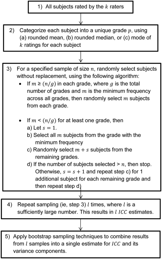
Flowchart showing the proposed sampling procedure, which uses the mean, median, or mode to help reduce the dependency of ICC on the distribution

4.2. Impact of sampling scheme on ICC

To assess performance of the proposed sampling method, non‐uniform datasets depicting convex and concave cases with varying degrees of non‐uniformity were simulated. ICC and variance estimates derived from the sampling scheme were compared with the estimates for the population from which the samples were derived as well as the standard paradigm which is the uniform distribution. If ICC and rater error variance estimates calculated from the sample are close to the uniform, then the sampling procedure is said to be capable of reducing their dependency on the distribution.

To facilitate this investigation, 10 000 data sets were simulated for each level of disagreement under extreme and mild concave and convex distributions with N = 300 subjects. The mean, median, and mode based on k = 8 ratings were calculated for each subject, and these statistics were then used to classify each subject into a unique grade. Samples of size n = 80 were then drawn as prescribed in Figure 2. As shown in Section 3.2, the choice of n = 80 as the sample size is appropriate as it provides ICC estimates reasonably similar to those when N = 300 is used. This sampling procedure was performed l = 20 times to reduce any sampling variability. Note that the extent of non‐uniformity among N = 300 will affect the degree of uniformity achieved in the samples generated. For mild concave or convex distributions, a nearly uniform sample is generated as an ample number of subjects is represented for each grade. However, a uniform sample is not achieved in cases of the extreme concave or convex distributions due to an insufficient number of subjects in at least one of the grades. Accordingly, the more non‐uniform sample for these cases has a total sample size closer to n = 80. Simulation results show that the extreme concave and convex distributions have sample sizes ranging from n = 80 − 83 for all 3 sampling methods across all 6 levels of disagreement. Conversely, wider ranges of the sample size are realized for mild concave and convex distributions, with n = 80 − 210; and for a nearly uniform distribution, the sample size can be close to N = 300. In this regard, having a larger sample size for more uniform distributions is not a source of difficulty because there is more available data from each grade to produce a uniform distribution. However, it is also possible for Figure 2 to be modified so that the sample size for a more uniform distribution is kept closer to n = 80 by imposing a restriction on how large the sample size should be.

As shown in Table 7 for extreme concave populations, the ICC values are higher than those of the samples generated from it for low levels of disagreement. However, as the levels of disagreement increase, sampling based on mean and median can produce higher ICC values when compared with those from the population. Additionally, for lower disagreements, ICC for samples based on all 3 methods are higher but closer to those for uniform data sets with N = 300. Specifically, the mode provides the smallest absolute difference from the uniform distribution across all 6 levels of disagreement. The same behavior is observed for mild concave cases. The interdecile ranges suggest that for lower levels of disagreement, approximately equal variability in the estimates are realized for the samples and full distributions. Also, the interdecile ranges of ICC estimates from all sampling methods are comparable to the uniform distribution.

Table 7.

Mean ICC (and interdecile range) across 10 000 simulations of uniform, convex and concave distributions with N = 300 and samples of at least size n = 80 from extreme and mild concave and convex distributions

Initial Distribution	Specificationsf		Levels of Disagreement
			Case 1	Case 2	Case 3	Case 4	Case 5	Case 6
Extreme concavea	Full distribution	N = 300	0.93 (0.01)	0.85 (0.02)	0.77 (0.02)	0.69 (0.02)	0.39 (0.05)	0.19 (0.04)
	Sampling method	Mean	0.91 (0.01)	0.81 (0.03)	0.75 (0.02)	0.72 (0.02)	0.56 (0.07)	0.31 (0.10)
		Median	0.91 (0.01)	0.81 (0.03)	0.72 (0.03)	0.65 (0.03)	0.36 (0.05)	0.28 (0.08)
		Mode	0.91 (0.01)	0.81 (0.02)	0.71 (0.03)	0.63 (0.03)	0.35 (0.05)	0.18 (0.04)
Mild concaveb	Full distribution	N = 300	0.93 (0.01)	0.84 (0.02)	0.76 (0.02)	0.68 (0.03)	0.38 (0.05)	0.19 (0.04)
	Sampling method	Mean	0.90 (0.01)	0.81 (0.02)	0.75 (0.02)	0.72 (0.02)	0.56 (0.07)	0.31 (0.09)
		Median	0.90 (0.01)	0.80 (0.02)	0.71 (0.03)	0.65 (0.03)	0.36 (0.05)	0.28 (0.08)
		Mode	0.90 (0.01)	0.80 (0.02)	0.70 (0.03)	0.61 (0.03)	0.34 (0.05)	0.18 (0.05)
Uniformc	Full distribution	N = 300	0.90 (0.01)	0.79 (0.02)	0.68 (0.03)	0.58 (0.03)	0.34 (0.05)	0.16(0.04)
Mild convexd	Full distribution	N = 300	0.82 (0.02)	0.65 (0.03)	0.51 (0.04)	0.39 (0.04)	0.26 (0.06)	0.11 (0.04)
	Sampling method	Mean	0.90 (0.01)	0.80 (0.03)	0.69 (0.06)	0.57 (0.08)	0.43 (0.10)	0.27 (0.08)
		Median	0.90 (0.01)	0.80 (0.03)	0.70 (0.04)	0.59 (0.07)	0.39 (0.10)	0.20 (0.09)
		Mode	0.90 (0.01)	0.79 (0.03)	0.68 (0.05)	0.58 (0.06)	0.36 (0.09)	0.18 (0.09)
Extreme convexe	Full distribution	N = 300	0.78 (0.02)	0.58 (0.04)	0.43 (0.04)	0.30 (0.04)	0.22 (0.06)	0.08 (0.04)
	Sampling method	Mean	0.86 (0.02)	0.72 (0.04)	0.58 (0.06)	0.47 (0.08)	0.39 (0.09)	0.25 (0.08)
		Median	0.86 (0.02)	0.72 (0.04)	0.59 (0.06)	0.47 (0.07)	0.32 (0.10)	0.16 (0.08)
		Mode	0.86 (0.02)	0.72 (0.04)	0.59 (0.06)	0.46 (0.07)	0.30 (0.10)	0.14 (0.08)

^aExtreme concave distribution indicates having 33%, 16.7%, 4%, 14%, and 32.3% of the subjects in grades 0, 1, 2, 3, and 4, respectively, for N = 300.

^bMild concave distribution indicates having 29.7%, 16.7%, 7.3%, 15.3%, and 31.0% of the subjects in grades 0, 1, 2, 3, and 4, respectively, for N = 300.

^cUniform distribution indicates having 20% of the subjects in grades 0, 1, 2, 3, and 4, N = 300.

^dMild convex distribution indicates having 6.7%, 24%, 36%, 27%, and 6.3% of the subjects in grades 0, 1, 2, 3, and 4, respectively, N = 300.

^eExtreme convex distribution indicates having 2.3%, 28.7%, 42.7%, 22.7%, and 3.6% of the subjects in grades 0, 1, 2, 3, and 4, respectively, N = 300.

^fSamples of size at least size n = 80 were selected using the sampling method.

For extreme convex distributions, Table 7 illustrates that the samples based on all 3 methods have higher ICC values compared with the population due to reduction in subject non‐uniformity. Upon sampling, ICC estimates are closer, but somewhat lower, relative to the standard paradigm for low levels of disagreement. However, although sampling based on the mean produces estimates that are higher than the uniform distribution, as the levels of disagreement increase, the interpretation would be comparable. Hence, it follows that an unreliable scale is not made to appear reliable by the sampling procedure. Similar trends are observed for the mild convex distribution and the skewed distributions.

Upon sampling, there is a reduction in subject variance for low levels of disagreement for the extreme and mild concave cases. However, as the disagreements become severe, ${\widehat{\sigma }}_a^2$ tends to be higher than the full distribution, with this being especially evident when using the mean. Additionally, ${\widehat{\sigma }}_a^2$ of the samples are higher when compared with the uniform distribution; however, sampling using the mode produces ${\widehat{\sigma }}_a^2$ that are closest to the uniform for all cases. On the other hand, sampling from extreme convex distributions leads to an increase in subject variance estimates for all levels of disagreement. Although there is an increase in ${\widehat{\sigma }}_a^2$, it does not exceed ${\widehat{\sigma }}_a^2$ from the uniform distribution except in the case of the mean for the most severe disagreement considered. Also, the absolute difference between the sample and the uniform ${\widehat{\sigma }}_a^2$ are minimal for all 3 sampling methods across all levels of disagreement. However, a reverse trend is observed for the mild convex distribution, where ${\widehat{\sigma }}_a^2$ for the samples slightly exceed that from the uniform distribution for all 3 sampling methods. In general, these results suggest that for extreme and mild convex distributions all 3 sampling methods provide subject variance estimates that are comparable to the standard paradigm. The interdecile ranges suggest that approximately similar ranges are achieved with sampling and uniform distribution for low levels of disagreement. The same behavior is likewise exhibited by the subject variance estimates for skewed distributions.

Furthermore, it was observed that the sampling method does not have a substantial impact on the rater error variance estimates when compared with the population from which it is derived, especially for lower levels of disagreement. Additionally, the estimates from the sample do not greatly differ from the uniform distribution, except for the mean with higher levels of disagreement; thus, no artificial improvement in reliability is introduced when sampling is performed. Furthermore, minimal disparities in interdecile range of the rater error variance estimates are observed when comparing the sample with the standard paradigm as well as the full distribution from where the samples were derived. This suggests that precision in estimates is not lost through sampling. The tables for ${\widehat{\sigma }}_a^2$ and ${\widehat{\sigma }}_b^2+{\widehat{\sigma }}_{\mathit{ab}}^2+{\widehat{\sigma }}_{ϵ}^2$ are available in Appendices A and B.

In general, simulations show that sampling increases ICC for the convex distributions while it decreases ICC for the concave distributions. For the convex distributions, the ICC does not exceed that of the standard uniform paradigm across all cases when median and mode are used. The mean, on the other hand, tends to produce higher ICC for severe levels of disagreement. Meanwhile, for the concave distributions, the ICC is not lower than that of the uniform distribution for all levels of disagreement when mode is used for sampling; while this behavior holds true for mean and median sampling methods only for low levels of disagreement. Furthermore, for lower levels of disagreement, the mean, median, and mode as sampling schemes provide approximately the same estimate. However, for higher levels of disagreement, the mean and median sampling techniques for the extreme concave distributions and mean sampling method for the extreme convex distributions tend to provide estimates that deviate from the general behavior described above. This behavior is illustrated in Appendix C. Based on the variance components, simulation results suggest that changes in ICC realized via sampling can mostly be attributed to corresponding changes in the study design component of subject variance ${{\widehat{\sigma }}_a}^2$ and not the rater error variance ${\widehat{\sigma }}_b^2+{\widehat{\sigma }}_{\mathit{ab}}^2+{\widehat{\sigma }}_{ϵ}^2$. Thus, sampling affects ICC by only reducing or minimizing dependencies caused by the study design through non‐uniform distributions. It, however, does not alter quality of the scale, as assessed by rater error, and thus does not make an unreliable scale look reliable.

5. APPLICATION

The impact of a non‐uniform distribution of subjects on ICC and the use of a sampling method to reduce this dependency of ICC are illustrated using the motivating example discussed in Section 1. As shown in Table 1, the distributions of subjects for the scales mimic the convex distributions. Hence, the calculated ICC may be downgraded relative to the uniform distribution as the simulation results suggest. The sampling method was implemented for this reliability study to reduce non‐uniformity without increasing the reliability with respect to the standard uniform paradigm. Detailed descriptions of the scale development process have been published.28

As shown through reasonably small interdecile ranges for ICC in Table 7, a target sample size of n = 80 subjects for k = 8 raters was used for the sampling method. Subsets of 80 to 115 subjects with minimal non‐uniformity across grades were randomly selected using the procedure described in Figure 2. The mean method was used to categorize subjects in each grade of the scale for the sampling method. The corresponding distribution of the sample for each scale is shown in Table 8, and it indicates that a completely uniform distribution was attained for the fine lines and skin roughness scales, while the other scales achieved a better extent of uniformity.

Table 8.

Distribution of subjects selected across the 5 photonumeric scales using the sampling method

Severity Scale	N0	N1	N2	N3	N4	Total
Fine lines	20%	20%	20%	20%	20%	115
Forehead lines	8%	23%	23%	23%	23%	83
Hand volume deficit	8%	26%	26%	26%	14%	81
Skin roughness	20%	20%	20%	20%	20%	80
Temple hollowing	16%	23%	23%	22%	16%	80

The sampling method based on the mean was repeated 20 times for each scale to reduce sampling variability, and the corresponding ICC, subject variance, and rater error variance estimates were calculated on each sample. The PROC MIANALYZE procedure in SAS 9.3 (Cary, NC) was used to combine results from the 20 samples. These results along with the interdecile range for the ICC values calculated from the 20 samples are provided in Table 9. The results based on the full set of subjects are also presented in the table.

Table 9.

ICC, subject variance, and rater error variance estimates for 5 scales using all subjects and sample

Severity Scale	All Subjects			Sample
	ICC	Subject variance	Rater error variance	ICC (interdecile range)	Subject variance (interdecile range)	Rater error variance (interdecile range)
Fine lines	0.61	1.09	0.39	0.76 (0.02)	1.72 (0.10)	0. 53 (0.06)
Forehead lines	0.82	1.14	0.21	0.86 (0.03)	1.47 (0.13)	0. 24 (0.05)
Hand volume deficit	0.73	0.65	0.23	0.82 (0.02)	1.14 (0.09)	0.25 (0.03)
Skin roughness	0.68	0.77	0.29	0.81 (0.02)	1.57 (0.09)	0. 36 (0.03)
Temple hollowing	0.68	0.68	0.29	0.81 (0.03)	1.41 (0.10)	0. 32 (0.05)

Note: The interdecile range is calculated using ICC values across the 20 simulations.

The results in Table 9 indicate that there is an increase in ICC for all scales when the sampling method is applied. It can be observed that the scales on fine lines and forehead lines are not affected by this sampling method because their corresponding ICC falls in the same range based on the threshold,30 and thus, no change in qualitative classification is realized; however, it is recognized that sampling leads to a much larger ICC estimate for the fine lines scale. On the other hand, for hand volume deficit, skin roughness, and temple hollowing, a noteworthy increase is obtained in the scale reliability classification after reducing the effect of distribution. In general, the substantial or better classification of the ICC after sampling suggests that all of the scales are reliable. Based on the variance components, the difference in ICC between all subjects and the sample can be attributed to the difference in subject variance, or more generally, the level of homogeneity of the subjects enrolled in the study. The rater error variance estimates are approximately equal between all subjects and the samples for all scales except fine lines. This implies that the sampling method reduced dependency on the distribution of subjects without a substantial effect on the rater error variance estimate; thus, the scale reliability index was not altered to appear artificially reliable. This application illustrates the use of the sampling method and its advantages. The reliability of the scale was also explored using the median and mode sampling methods. The results, although not shown, suggest that the ICC, subject variance, and rater error variance estimates from these methods were similar to those from the mean sampling. Furthermore, this implies that the use of any of the 3 sampling methods is able to provide more useful estimates without making the scale look artificially good. This procedure is deemed to be more appropriate in multiple‐scale studies, in which the different scales have a convex distribution for reasons expressed previously.

Additionally, the small interdecile ranges on ICC for all scales imply that a sample size smaller than 80 subjects would be sufficient for the sampling procedure. The results, although not shown, suggest that ICC estimates and interdecile ranges, for sample size as low as 50 subjects, are similar to the results shown in Table 9.

6. CONCLUSION

In reliability studies, ICC is one of the most commonly used methods to measure agreement. However, the estimate of this quantity is affected by the distribution of subjects and rater quality. Simulation results, as presented in this paper, suggest that for a fixed number of subjects, ICC from the convex distribution is smaller than ICC for the uniform distribution, which in turn is smaller than ICC for the concave distribution. The variance component estimates also show that the dissimilarity of ICC among distributions is attributed to the study design (ie, distribution of subjects) component of subject variability and not the scale quality component of rater error variability. The dependency of ICC on the distribution of subjects makes it difficult to compare results across reliability studies. Hence, it is proposed that reliability studies should be evaluated using the paradigm of a uniform distribution of subjects because of the objective standardization it provides for representing disagreement. Additionally, when the type of distribution is fixed, the results suggest that any increase in the number of subjects beyond a moderately large specification, such as n = 80, does not have an impact on ICC. This provides additional efficiency in study operations with respect to time and cost.

It may be operationally challenging to enroll a uniform distribution of subjects across grades, especially if some traits are uncommon, or in a multiple scales reliability study. The sampling method proposed reduces this non‐uniformity and produces ICC estimates that are closer to the standard paradigm of the uniform distribution. ICC estimates using the mean, median, and mode sampling methods for concave and convex distributions are comparable to the uniform distribution for low levels of disagreement; thus, any of the 3 sampling schemes may be used to derive reasonable ICC estimates. However, as the levels of disagreement increase in concave and convex distributions, the sampling method via the mode is a better measure to categorize, as it provides ICC that are closer to the uniform distribution. The advantages of the sampling method for convex distributions are also illustrated using a real‐life reliability study. Although higher ICC values were obtained using a sample of subjects compared with all subjects, the rater error variance estimates were approximately the same for the 2 cases.

We have not reported any results for the skewed distributions, but their behavior has been explored and is similar to that for the convex distribution; hence, sampling can be applied to skewed distributions to reduce dependency on the distribution.

APPENDIX A.

MEAN SUBJECT VARIANCE ESTIMATES, ${\widehat{\mathbf{\sigma }}}_{\mathit{a}}^{\mathbf{2}}$, AND INTERDECILE RANGE ACROSS 10 000 SIMULATIONS OF UNIFORM, CONVEX AND CONCAVE DISTRIBUTIONS WITH N = 300 AND SAMPLE OF AT LEAST SIZE n = 80 FROM EXTREME AND MILD CONCAVE AND CONVEX DISTRIBUTIONS

Initial Distribution	Specificationsf		Levels of Disagreement
			Case 1	Case 2	Case 3	Case 4	Case 5	Case 6
Extreme concavea	Full distribution	N = 300	2.43 (0.06)	2.08 (0.08)	1.76 (0.09)	1.47 (0.09)	0.91 (0.13)	0.39 (0.09)
	Sampling method	Mean	1.85 (0.06)	1.70 (0.11)	1.62 (0.07)	1.60 (0.07)	1.45 (0.24)	0.69 (0.25)
		Median	1.85 (0.06)	1.62 (0.09)	1.43 (0.10)	1.28 (0.08)	0.75 (0.10)	0.61 (0.20)
		Mode	1.85 (0.07)	1.59 (0.08)	1.36 (0.09)	1.16 (0.09)	0.67 (0.11)	0.33 (0.09)
Mild concaveb	Full distribution	N = 300	2.29 (0.06)	1.96 (0.08)	1.65 (0.09)	1.38 (0.09)	0.86 (0.12)	0.37 (0.09)
	Sampling method	Mean	1.74 (0.05)	1.64 (0.06)	1.59 (0.06)	1.59 (0.08)	1.41 (0.26)	0.67 (0.24)
		Median	1.74 (0.05)	1.53 (0.06)	1.36 (0.07)	1.26 (0.07)	0.75 (0.09)	0.60 (0.20)
		Mode	1.74 (0.05)	1.49 (0.07)	1.28 (0.07)	1.12 (0.07)	0.65 (0.09)	0.33 (0.09)
Uniformc	Full distribution	N = 300	1.70 (0.05)	1.44 (0.07)	1.21 (0.08)	1.00 (0.08)	0.63 (0.10)	0.27 (0.08)
Mild convexd	Full distribution	N = 300	0.93 (0.04)	0.77 (0.05)	0.63 (0.06)	0.50 (0.07)	0.33 (0.08)	0.15 (0.06)
	Sampling method	Mean	1.74 (0.08)	1.50 (0.15)	1.21 (0.23)	0.95 (0.23)	0.71 (0.21)	0.44 (0.16)
		Median	1.73 (0.08)	1.49 (0.11)	1.27 (0.16)	1.04 (0.21)	0.73 (0.21)	0.34 (0.17)
		Mode	1.72 (0.09)	1.46 (0.11)	1.23 (0.14)	1.01 (0.16)	0.67 (0.19)	0.32 (0.16)
Extreme convexe	Full distribution	N = 300	0.70 (0.04)	0.58 (0.05)	0.47 (0.05)	0.36 (0.06)	0.24 (0.06)	0.11 (0.05)
	Sampling method	Mean	1.24 (0.10)	1.01 (0.15)	0.82 (0.16)	0.67 (0.17)	0.54 (0.16)	0.37 (0.14)
		Median	1.24 (0.10)	1.04 (0.12)	0.85 (0.15)	0.68 (0.16)	0.47 (0.17)	0.24 (0.13)
		Mode	1.24 (0.10)	1.04 (0.12)	0.86 (0.14)	0.69 (0.16)	0.46 (0.17)	0.22 (0.14)

^a Extreme concave distribution indicates having 33%, 16.7%, 4%, 14%, and 32.3% of the subjects in grades 0, 1, 2, 3, and 4, respectively, N = 300.

^b Mild concave distribution indicates having 29.7%, 16.7%, 7.3%, 15.3%, and 31.0% of the subjects in grades 0, 1, 2, 3, and 4, respectively, N = 300.

^c Uniform distribution indicates having 20% of the subjects in grades 0, 1, 2, 3, and 4, N = 300.

^d Mild convex distribution indicates having 6.7%, 24%, 36%, 27%, and 6.3% of the subjects in grades 0, 1, 2, 3, and 4, respectively, N = 300.

^e Extreme convex distribution indicates having 2.3%, 28.7%, 42.7%, 22.7%, and 3.6% of the subjects in grades 0, 1, 2, 3, and 4, respectively, N = 300.

^f Samples of at least size n = 80 were selected using the sampling method.

APPENDIX B.

MEAN RATER ERROR VARIANCE ESTIMATES, ${\widehat{\mathit{\sigma }}}_{\mathit{b}}^{\mathbf{2}}+{\widehat{\mathit{\sigma }}}_{\mathit{ab}}^{\mathbf{2}}+{\widehat{\mathit{\sigma }}}_{\mathit{ϵ}}^{\mathbf{2}}$, AND INTERDECILE RANGE

Across 10 000 simulations of uniform, convex and concave distributions with N = 300 and sample of at least size n = 80 from extreme and mild concave and convex distributions.

Initial Distribution	Specificationsf		Levels of Disagreement
			Case 1	Case 2	Case 3	Case 4	Case 5	Case 6
Extreme concavea	Full distribution	N = 300	0.18 (0.01)	0.36 (0.03)	0.52 (0.04)	0.65 (0.04)	1.44 (0.12)	1.65 (0.10)
	Sampling method	Mean	0.19 (0.02)	0.39 (0.05)	0.53 (0.05)	0.61 (0.05)	1.13 (0.14)	1.51 (0.15)
		Median	0.19 (0.02)	0.38 (0.05)	0.55 (0.06)	0.68 (0.06)	1.37 (0.14)	1.61 (0.17)
		Mode	0.19 (0.02)	0.38 (0.05)	0.55 (0.06)	0.69 (0.06)	1.26 (0.11)	1.56 (0.11)
Mild concaveb	Full distribution	N = 300	0.18 (0.01)	0.37 (0.04)	0.53 (0.04)	0.66 (0.04)	1.40 (0.11)	1.61 (0.10)
	Sampling method	Mean	0.19 (0.02)	0.38 (0.05)	0.53 (0.05)	0.61 (0.05)	1.10 (0.14)	1.48 (0.15)
		Median	0.19 (0.02)	0.39 (0.05)	0.56 (0.06)	0.68 (0.05)	1.32 (0.13)	1.57 (0.17)
		Mode	0.19 (0.02)	0.39 (0.05)	0.56 (0.06)	0.70 (0.06)	1.24 (0.11)	1.54 (0.11)
Uniformc	Full distribution	N = 300	0.19 (0.02)	0.39 (0.04)	0.57 (0.05)	0.72 (0.05)	1.20 (0.11)	1.46 (0.09)
Mild convexd	Full distribution	N = 300	0.20 (0.02)	0.41 (0.04)	0.61 (0.05)	0.80 (0.06)	0.95 (0.09)	1.25 (0.09)
	Sampling method	Mean	0.18 (0.02)	0.37 (0.04)	0.54 (0.06)	0.71 (0.07)	0.93 (0.12)	1.19 (0.12)
		Median	0.19 (0.02)	0.38 (0.05)	0.55 (0.06)	0.72 (0.07)	1.13 (0.17)	1.33 (0.14)
		Mode	0.19 (0.02)	0.39 (0.05)	0.57 (0.06)	0.74 (0.08)	1.20 (0.17)	1.47 (0.16)
Extreme convexe	Full distribution	N = 300	0.20 (0.02)	0.42 (0.04)	0.63 (0.05)	0.82 (0.06)	0.88 (0.09)	1.19 (0.08)
	Sampling method	Mean	0.19 (0.02)	0.40 (0.05)	0.58 (0.06)	0.76 (0.07)	0.85 (0.11)	1.12 (0.12)
		Median	0.19 (0.02)	0.41 (0.05)	0.59 (0.06)	0.77 (0.07)	1.00 (0.14)	1.28 (0.13)
		Mode	0.20 (0.03)	0.41 (0.05)	0.60 (0.06)	0.80 (0.09)	1.07 (0.16)	1.39 (0.16)

^a Extreme concave distribution indicates having 33%, 16.7%, 4%, 14%, and 32.3% of the subjects in grades 0, 1, 2, 3, and 4, respectively, N = 300.

^b Mild concave distribution indicates having 29.7%, 16.7%, 7.3%, 15.3%, and 31.0% of the subjects in grades 0, 1, 2, 3, and 4, respectively, N = 300.

^c Uniform distribution indicates having 20% of the subjects in grades 0, 1, 2, 3, and 4, N = 300.

^d Mild convex distribution indicates having 6.7%, 24%, 36%, 27%, and 6.3% of the subjects in grades 0, 1, 2, 3, and 4, respectively, N = 300.

^e Extreme convex distribution indicates having 2.3%, 28.7%, 42.7%, 22.7%, and 3.6% of the subjects in grades 0, 1, 2, 3, and 4, respectively, N = 300.

^f Samples of at least size n = 80 were selected using the sampling method.

APPENDIX C.

EFFECT OF SAMPLING ON ICC GIVEN FULL EXTREME CONCAVE AND EXTREME CONVEX CASES

Note: The error bars represent the standard deviation OF THE 10 000 ICC estimates generated from the simulations.

Figure C1.

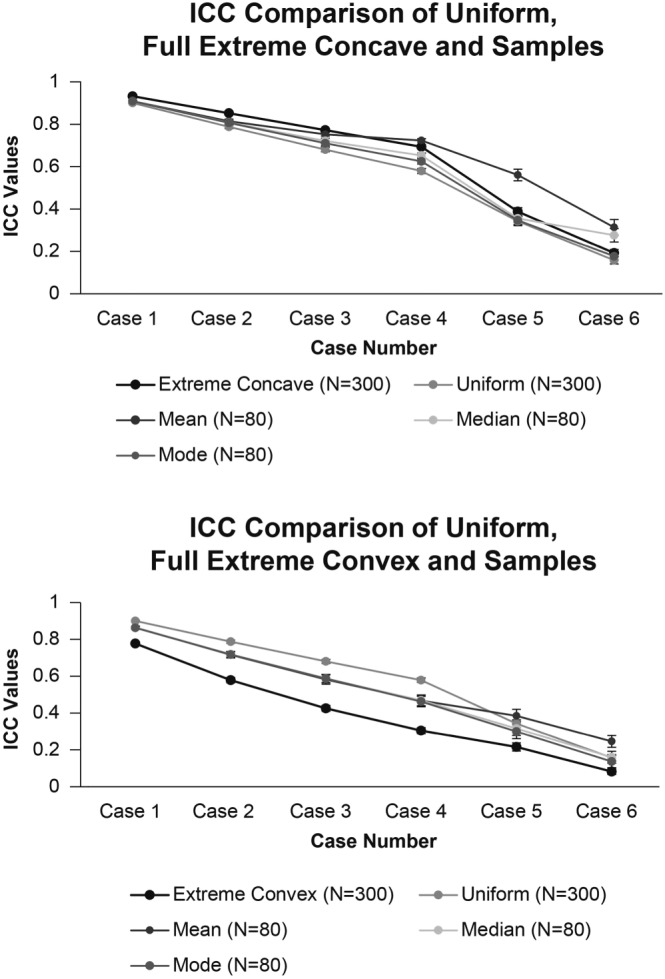
Effect of sampling on ICC given full extreme concave and extreme convex cases

Mehta S, Bastero‐Caballero RF, Sun Y, et al. Performance of intraclass correlation coefficient (ICC) as a reliability index under various distributions in scale reliability studies. Statistics in Medicine. 2018;37:2734–2752. 10.1002/sim.7679

REFERENCES

- 1. Shrout PE, Fleiss JL. Intraclass correlations: uses in assessing rater reliability. Psychol Bull. 1979;86(2):420‐428. [DOI] [PubMed] [Google Scholar]
- 2. Guidance for Industry : Patient‐reported outcome measures: use in medical product development to support labeling claims. Food and Drug Adminstration 2009. Available at: http://www.fda.gov/downloads/Drugs/Guidances/UCM193282.pdf. [DOI] [PMC free article] [PubMed]
- 3. Buchner L, Vamvakias G, Rom D. Validation of a photonumeric wrinkle assessment scale for assessing nasolabial fold wrinkles. Plast Reconstr Surg. 2010;126(2):596‐601. [DOI] [PubMed] [Google Scholar]
- 4. Kappes UP, Elsner P. Clinical and photographic scoring of skin aging. Skin Pharmacol Appl Skin Physiol. 2003;16(2):100‐107. [DOI] [PubMed] [Google Scholar]
- 5. Carruthers A, Carruthers J, Hardas B, et al. A validated grading scale for forehead lines. Dermatol Surg. 2008;34(Suppl 2):S155‐S160. [DOI] [PubMed] [Google Scholar]
- 6. Shoshani D, Markovitz E, Monstrey SJ, Narins DJ. The modified Fitzpatrick Wrinkle Scale: a clinical validated measurement tool for nasolabial wrinkle severity assessment. Dermatol Surg. 2008;34(Suppl 1):S85‐S91. [DOI] [PubMed] [Google Scholar]
- 7. Carruthers A, Carruthers J, Hardas B, et al. A validated grading scale for crow's feet. Dermatol Surg. 2008;34(Suppl 2):S173‐S178. [DOI] [PubMed] [Google Scholar]
- 8. Carruthers A, Carruthers J, Hardas B, et al. A validated grading scale for marionette lines. Dermatol Surg. 2008;34(Suppl 2):S167‐S172. [DOI] [PubMed] [Google Scholar]
- 9. Werschler WP, Fagien S, Thomas J, Paradkar‐Mitragotri D, Rotunda A, Beddingfield FC III. Development and validation of a photographic scale for assessment of lip fullness. Aesthet Surg J. 2015;35(3):294‐307. [DOI] [PMC free article] [PubMed] [Google Scholar]
- 10. Kane MA, Lorenc ZP, Lin X, Smith SR. Validation of a lip fullness scale for assessment of lip augmentation. Plast Reconstr Surg. 2012;129(5):822e‐828e. [DOI] [PubMed] [Google Scholar]
- 11. Rossi AB, Nkengne A, Stamatas G, Bertin C. Development and validation of a photonumeric grading scale for assessing lip volume and thickness. J Eur Acad Dermatol Venereol. 2011;25(5):523‐531. [DOI] [PubMed] [Google Scholar]
- 12. Carruthers A, Carruthers J, Hardas B, et al. A validated lip fullness grading scale. Dermatol Surg. 2008;34(Suppl 2):S161‐S166. [DOI] [PubMed] [Google Scholar]
- 13. Tsukahara K, Takema Y, Fujimura T, Moriwaki S, Kitahara T, Imokawa G. Determination of age‐related changes in the morphological structure (sagging) of the human cheek using a photonumeric scale and three‐dimensional surface parameters. Int J Cosmet Sci. 2000;22(4):247‐258. [DOI] [PubMed] [Google Scholar]
- 14. Larnier C, Ortonne JP, Venot A, et al. Evaluation of cutaneous photodamage using a photographic scale. Br J Dermatol. 1994;130(2):167‐173. [DOI] [PubMed] [Google Scholar]
- 15. Chung JH, Lee SH, Youn CS, et al. Cutaneous photodamage in Koreans: influence of sex, sun exposure, smoking, and skin color. Arch Dermatol. 2001;137(8):1043‐1051. [PubMed] [Google Scholar]
- 16. Carruthers A, Carruthers J, Hardas B, et al. A validated hand grading scale. Dermatol Surg. 2008;34(Suppl 2):S179‐S183. [DOI] [PubMed] [Google Scholar]
- 17. Shrout PE, Spitzer RL, Fleiss JL. Quantification of agreement in psychiatric diagnosis revisited. Arch Gen Psychiatry. 1987;44(2):172‐177. [DOI] [PubMed] [Google Scholar]
- 18. Streiner DL. Learning how to differ: agreement and reliability statistics in psychiatry. Can J Psychiatry. 1995;40(2):60‐66. [PubMed] [Google Scholar]
- 19. Spitznagel EL, Helzer JE. A proposed solution to the base rate problem in the kappa statistic. Arch Gen Psychiatry. 1985;42(7):725‐728. [DOI] [PubMed] [Google Scholar]
- 20. Grove WM, Andreasen NC, McDonald‐Scott P, Keller MB, Shapiro RW. Reliability studies of psychiatric diagnosis. Theory and practice. Arch Gen Psychiatry. 1981;38(4):408‐413. [DOI] [PubMed] [Google Scholar]
- 21. Byrt T, Bishop J, Carlin JB. Bias, prevalence and kappa. J Clin Epidemiol. 1993;46(5):423‐429. [DOI] [PubMed] [Google Scholar]
- 22. Cohen J. Weighted kappa: nominal scale agreement with provision for scaled disagreement or partial credit. Psychol Bull. 1968;70(4):213‐220. [DOI] [PubMed] [Google Scholar]
- 23. El‐Khorazaty JA, Koch G, Preisser J. The iterative proportional fitting algorithm for adjusted agreement in a non‐inferiority diagnostic clinical trial. Pharm Stat. 2014;13(3):173‐178. [DOI] [PubMed] [Google Scholar]
- 24. Carruthers A, Donofrio L, Hardas B, et al. Development and validation of a photonumeric scale for evaluation of static horizontal forehead lines. Dermatol Surg. 2016;42(suppl 1):S243‐S250. [DOI] [PMC free article] [PubMed] [Google Scholar]
- 25. Carruthers J, Donofrio L, Hardas B, et al. Development and validation of a photonumeric scale for evaluation of facial fine lines. Dermatol Surg. 2016;42(suppl 1):S227‐S234. [DOI] [PMC free article] [PubMed] [Google Scholar]
- 26. Jones D, Donofrio L, Hardas B, et al. Development and validation of a photonumeric scale for evaluation of volume deficit of the hand. Dermatol Surg. 2016;42(suppl 1):S195‐S202. [DOI] [PMC free article] [PubMed] [Google Scholar]
- 27. Donofrio L, Carruthers A, Hardas B, et al. Development and validation of a photonumeric scale for evaluation of facial skin texture. Dermatol Surg. 2016;42(suppl 1):S219‐S226. [DOI] [PMC free article] [PubMed] [Google Scholar]
- 28. Carruthers J, Jones D, Hardas B, et al. Development and validation of a photonumeric scale for evaluation of volume deficit of the temple. Dermatol Surg. 2016;42(suppl 1):S203‐S210. [DOI] [PMC free article] [PubMed] [Google Scholar]
- 29. Fleiss JL, Cohen J. The equivalence of weighted kappa and the intraclass correlation coefficient as measure of reliability. Educ Psychol Meas. 1973;33(3):613‐619. [Google Scholar]
- 30. Landis JR, Koch GG. The measurement of observer agreement for categorical data. Biometrics. 1977;33(1):159‐174. [PubMed] [Google Scholar]
- 31. Barnhart HX, Haber MJ, Lin LI. An overview on assessing agreement with continuous measurements. J Biopharm Stat. 2007;17(4):529‐569. [DOI] [PubMed] [Google Scholar]
- 32. Bland JM, Altman DG. Statistical methods for assessing agreement between two methods of clinical measurement. Lancet. 1986;1(8476):307‐310. [PubMed] [Google Scholar]
- 33. Quan H, Shih WJ. Assessing reproducibility by the within‐subject coefficient of variation with random effects models. Biometrics. 1996;52(4):1195‐1203. [PubMed] [Google Scholar]
- 34. Lin LI. A concordance correlation coefficient to evaluate reproducibility. Biometrics. 1989;45(1):255‐268. [PubMed] [Google Scholar]
- 35. Chen CC, Barnhart HX. Comparison of ICC and CCC for assessing agreement for data without and with replications. Comput Stat Data Anal. 2008;53(2):554‐564. [Google Scholar]
- 36. Barnhart HX, Haber M, Song J. Overall concordance correlation coefficient for evaluating agreement among multiple observers. Biometrics. 2002;58(4):1020‐1027. [DOI] [PubMed] [Google Scholar]
- 37. Bartko JJ. Measurement and reliability: statistical thinking considerations. Schizophr Bull. 1991;17(3):483‐489. [DOI] [PubMed] [Google Scholar]