Methods for evidence synthesis in the case of very few studies

Abstract

In systematic reviews, meta‐analyses are routinely applied to summarize the results of the relevant studies for a specific research question. If one can assume that in all studies the same true effect is estimated, the application of a meta‐analysis with common effect (commonly referred to as fixed‐effect meta‐analysis) is adequate. If between‐study heterogeneity is expected to be present, the method of choice is a meta‐analysis with random effects. The widely used DerSimonian and Laird method for meta‐analyses with random effects has been criticized due to its unfavorable statistical properties, especially in the case of very few studies. A working group of the Cochrane Collaboration recommended the use of the Knapp‐Hartung method for meta‐analyses with random effects. However, as heterogeneity cannot be reliably estimated if only very few studies are available, the Knapp‐Hartung method, while correctly accounting for the corresponding uncertainty, has very low power. Our aim is to summarize possible methods to perform meaningful evidence syntheses in the situation with only very few (ie, 2‐4) studies. Some general recommendations are provided on which method should be used when. Our recommendations are based on the existing literature on methods for meta‐analysis with very few studies and consensus of the authors. The recommendations are illustrated by 2 examples coming from dossier assessments of the Institute for Quality and Efficiency in Health Care.

1. INTRODUCTION

In systematic reviews (SRs), meta‐analyses are routinely applied to summarize the results of the relevant studies for a specific research question.1 In this context, a prerequisite is to adequately assess between‐study heterogeneity. If heterogeneity is too large for a meaningful pooling of the available study results, no quantitative summary of the study results should be performed. If one can assume that in all studies the same true effect is estimated, ie, there is no true heterogeneity, the application of a meta‐analysis with common effect (commonly referred to as fixed‐effect meta‐analysis) is adequate. If a certain amount of heterogeneity is expected but nevertheless the pooling of study results for a joint interpretation seems to be sensible, the method of choice is a meta‐analysis with random effects.

A method for meta‐analyses with random effects was proposed by DerSimonian and Laird,2 which has become the standard method for this type of analyses. However, for some time now, this method has been criticized due to its unfavorable statistical properties, especially in the case of only (very) few available studies.3, 4, 5 A working group of the Cochrane Collaboration recommended the use of the Knapp‐Hartung method,6, 7 which was around the same time independently proposed by Sidik and Jonkman8 as new standard approach for random‐effects (RE) meta‐analysis.9

However, an unsolved problem in this context is the case of very few (ie, 2‐4) studies.10 As heterogeneity cannot be reliably estimated if only very few studies are available,11 the Knapp‐Hartung method, while correctly accounting for the corresponding uncertainty, has very low power and leads to wide confidence intervals (CIs).12 In practice, it can happen that the Knapp‐Hartung method yields a statistically not significant pooled effect estimate when combining 2 statistically significant studies with effects pointing into the same direction. This in first place counterintuitive result follows from the application of a model with random effects in the case of insufficient data for the reliable estimation of between‐study heterogeneity. Although some efforts have been made to evaluate the Knapp‐Hartung method with an ad hoc variance correction in the context with few studies,13 some uncertainty remains in which situations the application of the variance correction is advisable.

The evidence synthesis in the case of very few studies is therefore challenging as it is on the one hand often difficult to make a compelling case for a common‐effect (CE) meta‐analysis and on the other hand difficult to estimate the level of heterogeneity reliably. In this paper, we review a range of alternative methods to perform meaningful evidence syntheses in the situation with very few studies. Some general recommendations are provided on which method should be used when. Some examples illustrating the recommendations are provided.

The paper is organized as follows. After a brief description of the generic theoretical meta‐analysis models with common effect, fixed effects, and random effects in Section 2, we summarize the main available qualitative and quantitative methods for evidence synthesis in the case of very few studies in Section 3. In Section 4, we present 2 examples illustrating the limitations of the available meta‐analytic approaches when only very few studies are available. A short discussion follows in Section 5. We conclude with general recommendations on meaningful evidence syntheses in the case of very few studies. Our recommendations are based on the existing literature on methods for meta‐analysis with very few studies and expert consensus.

2. GENERIC MODELS FOR META‐ANALYSIS

2.1. Common‐effect model

When the pooling of the study results seems to be meaningful, the simplest meta‐analytic approach is the CE model assuming that the true treatment effects are all the same in all studies included. Let y _i be the observed treatment effect in study i for i = 1, …, k, θ _CE the common true treatment effect measured in terms of an appropriate effect measure, and ε_i a random variable describing the sampling error of study i. Then the CE model is given by

$$y_i={\mathit{\theta }}_{\mathit{CE}}+{\epsilon }_i,{\epsilon }_i~{\rm N}\left(0,v_i\right),\mathrm{Var}\left(y_i\right)=v_i.$$

The main parameter of interest is given by θ _CE, the common true treatment effect.

It should be noted that this model is usually referred to as “fixed‐effect model” rather than “CE model.” However, to avoid confusion with the fixed‐effects (FE) model by Laird and Mosteller,14 which will be introduced in the next subsection, we use the term “CE model” model here throughout. Other terms for the CE model are given by “equal‐effect model” or, misleadingly, also “fixed‐effects model.”

The major limitation of the CE model is the basic assumption that all studies estimate the same effect. This assumption is frequently challenged in practice. Applying a CE model in a situation where the basic CE assumption is violated may lead to far too narrow CIs and substantially increased type 1 error.10 Usually, whenever heterogeneity cannot be excluded, the CE model should not be used.

2.2. Fixed‐effects model

Less stringent than the CE assumption is the assumption that all studies have different expected effects. In the FE model according to Laird and Mosteller,14 it is assumed that each study has its own true treatment effect. However, the studies are, in contrast to the RE model, not considered as a random sample of all possible studies. The treatment effects of the studies are considered as fixed effects, which means that, strictly speaking, conclusions from a FE model apply to just the studies analyzed and not to all studies that are theoretically possible.

Let y _i be the observed treatment effect in study i for i = 1, …, k, θ _i the true treatment effect of study i, and ε_i a random variable describing the sampling error of study i. Then the FE model is given by

$$y_i={\mathit{\theta }}_i+{\epsilon }_i,{\epsilon }_i~{\rm N}\left(0,v_i\right),\mathrm{Var}\left(y_i\right)=v_i.$$

The main parameter of interest is given by an appropriate function of the treatment effects θ _i, in the simplest case with equal importance of all studies the unweighted average

$${\theta }_{\mathit{FE}}=\frac{1}{k}{\sum }_{i=1}^k{\theta }_i.$$

If studies are felt to have different importance, we can specify different weights to each study and define the average effect by using a weighted mean. One pragmatic option to specify weights is given by the sample sizes of the studies. In the case of equal true study effects, the FE model simplifies to the CE model.

2.3. Random‐effects model

In the RE model, it is assumed that the treatment effects vary randomly from study to study according to a random distribution (commonly and without further justification assumed to be normal) and the studies included in the meta‐analysis represent a random sample of theoretically possible studies. Let y _i be the observed treatment effect in study i for i = 1, …, k, θ _i the true treatment effect of study i, θ _RE the mean of the distribution of true treatment effects θ _i, δ_i a random variable describing the between‐study variation, and ε_i a random variable describing the within‐study variation; the random variables δ_i and ε_i are assumed to be independent. Then the RE model is given by

$$y_i={\theta }_i+{\epsilon }_i,{\theta }_i={\mathit{\theta }}_{\mathit{RE}}+{\delta }_i,{\epsilon }_i~{\rm N}\left(0,v_i\right),{\delta }_i~{\rm N}\left(0,{\tau }^2\right),\mathrm{Var}\left(y_i\right)=v_i+{\tau }^2.$$

The main parameters of interest are given by θ _RE, the mean of the distribution of true treatment effects, and the between‐study variation τ ² (heterogeneity).

The RE model encompasses within‐study (ν _i) as well as between‐study variation (τ ²), whereas the CE model includes only the within‐study variation. If the between‐study variation is zero (τ ² = 0), the RE model simplifies to the CE model.

3. METHODS FOR EVIDENCE SYNTHESIS

3.1. Qualitative evidence synthesis

In the situation of large heterogeneity where the pooling of study results seems to be not meaningful, no quantitative summary of the study results should be performed. If the heterogeneity can be explained and it is possible to divide the available data into fairly homogenous subsets (studies with certain conditions or subgroups within studies), separate meta‐analyses can be performed within the homogenous subsets. However, in meta‐analyses with very few studies, heterogeneity between studies can typically not be explained due to the small number of studies if only summary data are available. In this case, the only choice is a qualitative evidence synthesis in which the single study results are presented together with the results of the heterogeneity evaluations.

Nevertheless, there are situations in which clear statements on the effect direction are possible. For example, in the case of 2 or more statistically significant studies of high quality (ie, randomized controlled trials with low risk of bias) with estimated effects in the same direction demonstrating beneficial effects, the clear statement can be made that a benefit of the considered intervention is proven. However, due to unexplained heterogeneity, a meaningful quantification of the effect size is not possible.

An example where this approach is useful is given by the benefit assessment of new drugs according to the German Act on the Reform of the Market for Medicinal Products (Gesetz zur Neuordnung des Arzneimittelmarktes, AMNOG) in Germany. Here, one defined category to describe the extent of added benefit is given by a “nonquantifiable” added benefit.15 In a situation as described above, the result of the benefit assessment would be a proof of added benefit with nonquantifiable extent.

3.2. Meta‐analysis assuming a common effect

In cases where the pooling of the study results seems to be meaningful, the simplest meta‐analytic approach is given by the CE model assuming a true common treatment effect in all studies included in the meta‐analysis. For continuous endpoints, the usual standard estimation approach is the inverse variance method, where the pooled effect estimate is calculated by a weighted average of the effect estimates in each study and the weight given to each study is chosen to be the inverse of the estimated variance of the corresponding effect estimate, ie,

$${\widehat{\theta }}_{\mathit{CE}}=\frac{{\sum }_{i=1}^k{y}_i{w}_{i,\mathit{CE}}}{{\sum }_{i=1}^k{w}_{i,\mathit{CE}}}\text{with}{w}_{i,\mathit{CE}}=\frac{1}{{\widehat{v}}_i}.$$

The (1−α) CI for the common effect in the CE meta‐analysis is calculated by

$${\widehat{\theta }}_{\mathit{CE}}\pm z_{1-\frac{\alpha }{2}}\sqrt{\frac{1}{{\sum }_{i=1}^k{w}_{i,\mathit{CE}}},}$$ (1)

where z _q is the q‐quantile of the standard normal distribution. By using this approach, larger studies having smaller standard errors (SEs) are given more weight than smaller studies having larger SEs.1 In the case of binary endpoints, this approach is also applicable but not recommended due to undesirable statistical properties (see section 3.5).

3.3. Meta‐analysis assuming fixed effects

In a meta‐analysis with fixed effects and equal importance of all studies the average effect is estimated by means of the simple unweighted average of the estimated study effects,14 ie,

$${\widehat{\theta }}_{\mathit{FE}}=\frac{1}{k}{\sum }_{i=1}^k{y}_i.$$

The (1−α) CI for the pooled effect in the FE meta‐analysis is calculated by

$${\widehat{\theta }}_{\mathit{FE}}\pm z_{1-\frac{\alpha }{2}}\frac{1}{k^2}\sqrt{{\sum }_{i=1}^k{\widehat{v}}_i}.$$

In the case we think that the studies have different importance, we can specify different weights to each study and estimate the average effect by using a weighted mean. One pragmatic option to specify weights is given by the sample sizes of the studies.

However, the specification of study weights by the investigator is problematic in practice. Usually, larger studies with smaller SEs are more reliable than smaller studies with larger SEs. But specifying weights according to SEs would lead again to the usual CE meta‐analysis. Rice et al16 argue that the usual point and interval estimates of the CE model under standard conditions are also valid estimates for a weighted average effect under the FE model. However, a disadvantage of this approach is that the theoretical parameter of interest (θ _FE) is dependent on the sample size of the considered studies. In practice, the FE meta‐analysis has not gained acceptance in medical statistics. Obvious theoretically “correct” weights for the studies in a meta‐analysis to define a meaningful parameter of interest are not available in general. On the other hand, the estimation of the average effect by means of the simple unweighted average of the estimated study effects appears not to be helpful in the typical situation of a SR regarding a medical intervention.

3.4. Meta‐analysis assuming random effects

For a long time, the standard method for meta‐analyses with random effects was given by the method described in the seminal paper by DerSimonian and Laird.2 Using this approach, the mean of the distribution of true treatment effects is estimated by

$${\widehat{\theta }}_{\mathit{RE}}=\frac{\frac{1}{n}{\sum }_{i=1}^k{y}_i{w}_{i,\mathit{RE}}}{\frac{1}{n}{\sum }_{i=1}^k{w}_{i,\mathit{RE}}}\text{with}{w}_{i,\mathit{RE}}=1/\left({\widehat{v}}_i+{\widehat{\tau }}^2\right).$$

DerSimonian and Laird2 discussed 3 methods to estimate τ: noniterative method of moments procedure as well as iterative maximum likelihood and restricted maximum likelihood methods. The suggestion of the authors to use the method of moments estimator is based on comparability of results and its simplicity. A CI for the random effects mean can be constructed by using Equation (1) and replacing w _i,CE with w _i,RE.

For some time, the DerSimonian‐Laird method is criticized due to its unfavorable statistical properties, especially in the case of few available studies.4, 5, 9, 10, 17, 18, 19 The main problem of the DerSimonian‐Laird method is that the uncertainty of the estimation of the between‐study and within‐study variance is ignored.4, 12, 18 A number of alternative methods to perform meta‐analyses with random effects have been proposed (see below) including various methods to estimate the between‐study variance.19 Veroniki et al19 recommended the use of the Paule‐Mandel method20 instead of the method of moments procedure to estimate the between‐study variance in practice.

A working group of the Cochrane Collaboration recommended the use of the Knapp‐Hartung method6, 7 in combination with the Paule‐Mandel estimator for the between‐study variance instead of the DerSimonian‐Laird method as new standard approach in RE meta‐analysis.9 Using this approach, estimation of the mean of the distribution of true treatment effects is unchanged. However, a different (1−α) CI for the mean of the distribution of true treatment effects in the RE meta‐analysis is utilized

$${\widehat{\theta }}_{\mathit{RE}}\pm t_{k-1,1-\frac{\alpha }{2}}\sqrt{\frac{{\sum }_{i=1}^k{w}_{i,\mathit{RE}}\left(y_i-{\widehat{\theta }}_{\mathit{RE}}\right)2}{\left(k-1\right){\sum }_{i=1}^k{w}_{i,\mathit{RE}}},}$$

where t _m,q is the q‐quantile of the t‐distribution with m degrees of freedom. As is apparent from the simulations presented in Friede et al,21 the coverage probabilities of the CIs are not markedly improved by use of the Paule‐Mandel estimator in comparison to the DL estimator in meta‐analyses with only few studies.

In cases with very homogeneous study results, the variance of the estimated mean of the distribution of true treatment effects according to the Knapp‐Hartung method may turn out to be arbitrarily small, which means that the CI is misleadingly narrow.6, 22 For this case, a simple ad hoc variance correction was proposed,7 which is given by

$$\mathrm{Var}\left({\widehat{\theta }}_{\mathit{RE}}\right)=max\left[\frac{1}{{\sum }_{i=1}^k{w}_{i,\mathit{RE}}},\frac{{\sum }_{i=1}^k{w}_{i,\mathit{RE}}\left(y_i-{\widehat{\theta }}_{\mathit{RE}}\right)2}{\left(k-1\right){\sum }_{i=1}^k{w}_{i,\mathit{RE}}}\right].$$

This variance correction avoids arbitrarily narrow CIs. Röver et al13 recommended the use of the variance correction, especially in the case of very few studies. However, in the extreme case of only k = 2 studies, the Knapp‐Hartung method with variance correction tends to be over‐conservative. Therefore, the situation of k = 2 studies was considered as effectively unsolved.10, 13 Wiksten et al22 recommended to apply the RE meta‐analysis based upon the Knapp‐Hartung method and to conduct a sensitivity analysis using the CE meta‐analysis in practice to avoid misleading results.

3.5. Methods for binary endpoints

Under the CE model, well‐established statistical methods, eg, Mantel‐Haenszel and Peto methods, are available for the meta‐analysis of binary endpoints.23, 24, 25 In contrast, several evaluations show that the standard inverse‐variance method can perform very poorly with binary endpoints both under the CE and the RE model; especially in the case of rare events.24, 26 Accordingly, other meta‐analytic methods should be considered under the RE model.

A distinctive and frequently overlooked advantage of binary endpoints is that individual patient data (IPD) for endpoint and intervention are readily available if information on the studies' 2 × 2 tables is given.27 Even if only effect estimates together with CI or SEs are given, 2 × 2 tables can be reconstructed by using the method of Di Pietrantonj.28 The application of standard inverse‐variance meta‐analytic methods based upon summary measures (models with common effect or random effects) is probably not efficient in these cases, and methods that use the full IPD information should be preferred.25, 29 Essentially all of these models fall into the class of logistic regression models for correlated data, where the single models differ by model formulation and the respective estimation procedures, an overview is given by Agresti.30 Prominent class members are generalized linear mixed models with penalized quasi‐likelihood or numerical integration by Gaussian quadrature, marginal models with generalized estimation equations, conditional models with partial likelihood, and models with closed‐form likelihood functions such as the beta‐binomial model.31, 32 These models are suitable for zero and double‐zero trials and allow the consideration of trial duration as well as other covariates on trial level. Additionally, models with fixed study effects are possible, ie, the standard logistic regression model with the study effect as a categorical covariate. For these methods, a number of simulation studies are available.31, 33, 34, 35, 36 Under the assumption that the situation with few studies is similar to the situation with few observed events, beta‐binomial models might have favorable properties,31 but additional simulation evidence is needed before drawing definite conclusions here.

3.6. Individual patient data

Meta‐analyses of IPD are in general more reliable than meta‐analyses based upon aggregate data.37 If IPD are available, the use of linear mixed models for continuous endpoints and survival time methods for time‐to‐event endpoints offer the same advantages as the use of generalized linear mixed models for binary data (see Section 3.5) or count data. Thus, an effort should be made to obtain access to IPD, especially in the case of very few studies. However, in practice, access to IPD is frequently not possible for a variety of reasons.

3.7. Bayesian methods

A competitive alternative to frequentist methods of meta‐analysis is given by Bayesian methods. A general framework on how Bayesian RE models can be applied in practice is given by Smith et al.38 In a Bayesian analysis, often noninformative prior distributions are chosen for the unknown parameters. Inferences about the effects of interest are made by integrating out the unknown parameters from the joint distribution of the prior and the likelihood. Bayesian methods can have advantages compared with frequentist methods in specific data situations such as rare events.39 Fitting the models presented here does not require application of MCMC sampling, but can be done by application of robust approximation methods.40, 41 Furthermore, the practical application is supported by available R packages such as bayesmeta.21

In the situation of few studies, the main difficulty is given by the fact that heterogeneity cannot be reliably estimated. The use of Bayesian methodology allows the inclusion of prior knowledge about the heterogeneity parameter in the form of (weakly) informative prior distributions in the analysis to improve statistical inference on the effects of interest. This approach is described by Friede et al12, 21 in meta‐analyses of few small studies in rare diseases.

To apply Bayesian methods with informative priors for the between‐study heterogeneity, reliable information on the prior distribution of the unknown parameters is required. By using empirical data from the Cochrane Database of Systematic Reviews, Turner et al42 and Rhodes et al43 provide predictive distributions for the expected between‐study variance in different settings (defined by outcome type, intervention comparison type, and medical area), which can be used as informative prior distributions in future meta‐analyses.

The use of informative prior distributions in Bayesian RE meta‐analyses seems to be a promising approach for special data situations. A discussion of sensible choices of prior distributions for the heterogeneity parameter can for instance be found in Spiegelhalter et al44 In the setting with (very) few small studies as frequently encountered in rare diseases, the use of half‐normal priors with scale 0.5 and 1 were suggested, which led to an acceptable compromise in terms of coverage probabilities and lengths of the resulting credibility intervals in the settings considered.12, 21 However, the choice of prior information in Bayesian meta‐analyses with very few studies can have substantial effects on the final results.25 Moreover, it cannot be expected that reliable prior information is available for all intervention types and all medical disciplines, so that this approach cannot be routinely applied in all future meta‐analyses.

3.8. Other methods

Several alternative methods have been proposed in the literature such as the combination of exact confidence curves (also called P‐value functions or confidence distributions), which contains the combination of P‐values and CIs as special cases,45 or nonparametric approaches based upon permutation tests and resampling.18 However, none of the existing approaches solves the main problem that heterogeneity cannot be reliably estimated if only few studies are available. Guolo and Varin18 recommended the use of the Knapp‐Hartung method if a sufficient number of studies is available and that very complex and computer‐intensive methods should be avoided. In the case of few studies, Guolo and Varin18 proposed to apply various methods and draw corresponding conclusions from the comparison of the results of different methods.

4. EXAMPLES

For illustration, we consider 2 examples coming from dossier assessments of the Institute for Quality and Efficiency in Health Care.46, 47 In both examples, no pooling of the study results had been performed in the dossier assessments due to large heterogeneity. Nevertheless, both examples can be used to illustrate the limitations of the available meta‐analytic approaches in the case of very few studies.

4.1. Example 1: Belatacept after kidney transplant

In the first example, the added benefit of belatacept compared with ciclosporin A in combination with corticosteroids and mycophenolate mofetil as the appropriate comparator therapy for prophylaxis of graft rejection in adults receiving a renal transplant was assessed.46 Only k = 2 studies were available in this assessment. One of the considered patient relevant outcomes was the time‐to‐event endpoint “renal insufficiency in chronic kidney disease stage 4/5.” Both studies were statistically significant demonstrating a clear added benefit of belatacept. The Knapp‐Hartung method yields a very wide 95% CI due to the insufficient data to estimate the heterogeneity reliably (see Figure 1). Considering the result of 2 statistically significant studies demonstrating a clear added benefit of belatacept, the Knapp‐Hartung method is over‐conservative in this example. A decision that no added benefit of belatacept is proven based upon the results of the Knapp‐Hartung method would be critical, because a merely qualitative evidence synthesis would yield a clear added benefit. On the other hand, under the assumption of heterogeneous effects, the statistically significant result of the DerSimonian‐Laird method is unreliable due to the potentially increased type‐1 error (or, equivalently, reduced coverage probability of the CIs). The use of Bayesian RE meta‐analysis represents an alternative to these methods as the intervals are much shorter than the uninformative Knapp‐Hartung interval but yet considerably wider than the DerSimonian‐Laird interval. As this example demonstrates, however, prespecification of the prior distribution for the between‐study variation τ ² is important when interpreting the intervals in a frequentist sense as a hypothesis test because the application of the half‐normal prior with scale 0.5 for τ leads to a statistically significant pooled effect estimate in contrast to the half‐normal prior with scale 1 (see Figure 1).

Figure 1.

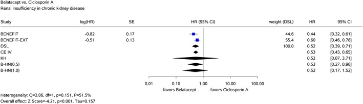
Results of the common‐effects model with inverse‐variance method (CE IV) and the random‐effects model with the DerSimonian‐Laird method (DSL), the Knapp‐Hartung method (KH), and Bayesian method using half‐normal priors for τ with scales 0.5 (B‐HN(0.5)) and 1.0 (B‐HN(1.0)) for the belatacept example [Colour figure can be viewed at http://wileyonlinelibrary.com]

4.2. Example 2: Sipuleucel‐T in prostate cancer

In the second example, the added benefit of sipuleucel‐T compared with the appropriate comparator therapy for treatment of asymptomatic or minimally symptomatic metastatic (nonvisceral) castrate‐resistant prostate cancer in male adults in whom chemotherapy is not yet clinically indicated was assessed.47 In this example, k = 3 relevant studies were available. One of the considered patient relevant binary outcomes was the side effect fever. In all 3 studies, there was, based upon exact statistical inference, a statistically significant difference between the treatment groups to the disadvantage of sipuleucel‐T; the effects were therefore clearly in the same direction (see Figure 2). There was an outcome‐specific high risk of bias for all studies. Hence, there was an indication of greater harm from sipuleucel‐T.47 However, the Knapp‐Hartung method again yields a very wide 95% CI due to the insufficient data to estimate the heterogeneity reliably. Thus, even in the case of k = 3 studies, the Knapp‐Hartung method can be over‐conservative in that it yields very long, uninformative CIs. The inverse‐variance method and the beta‐binomial model yield very similar results in this example (see Figure 2). If the CE assumption can be justified, both methods seem to deliver useful pooled effect estimates supporting an about 2.5‐fold increased risk of fever in patients in the sipuleucel‐T arm. If the CE assumption is rejected, a qualitative evidence synthesis would also lead to the conclusion that fever is more frequent in patients in the sipuleucel‐T arm because all studies are statistically significant in the same direction to the disadvantage of sipuleucel‐T (without quantification of the effect size). The same conclusion could be made on the basis of the Bayesian RE meta‐analyses using the half‐normal priors for τ with scale 0.5 and 1 (see Figure 2).

Figure 2.

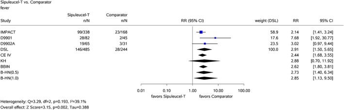
Results of the common‐effects model with inverse‐variance method (CE IV), the random‐effects model with the DerSimonian‐Laird method (DSL) and the Knapp‐Hartung method (KH), the beta‐binomial model (BBIN), and Bayesian method using half‐normal priors for τ with scales 0.5 (B‐HN(0.5)) and 1.0 (B‐HN(1.0)) for the sipuleucel‐T example [Colour figure can be viewed at http://wileyonlinelibrary.com]

5. DISCUSSION

No satisfactory universal method is currently available to perform meta‐analyses in the case of very few studies. The major limitation of the CE model is the basic assumption that all studies estimate the same effect. This assumption is frequently questionable in practice. It is, however, often overlooked that the interpretation of the outcome of the meta‐analysis may also be challenging as soon as we have to acknowledge that 2 studies that were considered combinable in the beginning turn out to support different true treatment effects. Applying a CE meta‐analysis in a situation where the basic assumption of a true common treatment effect is violated may lead to substantially increased type 1 error (or, equivalently, reduced coverage probability of the CIs). In general, as soon as observed results indicate that the available studies are not sufficiently homogeneous, the CE model should not be used for evidence synthesis.

However, in situations with only one single study, results of this study are interpreted and conclusions are made for the considered population. This analysis can be considered as a degenerated CE meta‐analysis with full weight given to the available study. However, this study is just a sample (with sample size k = 1) of all studies, which are theoretically possible. If heterogeneity of all theoretically possible studies cannot be excluded, a better approach to generalize the results to the whole population is given by a meta‐analysis with random effects, which, however, cannot be performed by using frequentist methods if there is only a single study. Using the same logic in the case of k = 2 studies would lead to the application of the CE or the FE model. However, in the case of 2 or more studies, we can technically investigate heterogeneity and because this is a basic step in SRs and important for conclusions referring to the whole population, we try to assess heterogeneity even if heterogeneity cannot reliably be estimated in the case of very few studies. It is interesting thus to compare the approach of a meta‐analysis with the assessment of consistency within a single study, which is usually done during the assessment of the results of a single study over all relevant endpoints (benefit/risk in drug approval or benefit assessment in health technology assessment).

To avoid a large discontinuity in making conclusions from k = 1 study or k = 2 studies, the use of the CE or the FE model should be considered. The use of the FE model would have the advantage that the strong CE assumption is not required. However, the unweighted FE model cannot be recommended because large studies provide in general better evidence than small studies. The use of the weighted FE model with weights inversely proportional to the variances of the effect estimates leads to the same estimator as the CE model but has the disadvantage that the theoretical parameter of interest is dependent on the sample size of the considered studies. Moreover, the difference between the CE and the FE model will be frequently not understood in practice. Therefore, we recommend not to use the FE model but to consider the use of the CE model. It should be carefully assessed whether an amount of heterogeneity should be expected, which would make the usual CE model unreliable. Situations where the application of the CE model seems to be appropriate are given by 2 studies with identical design (so‐called twin studies) or with large estimated effects and negligible between‐study heterogeneity. In summary, in the situation with very few studies, the simple CE model should be applied more frequently compared with situations with a large number of studies where the RE model is in general the model of choice.

Besides the problem that between‐study heterogeneity cannot be estimated reliably, meta‐analyses of very few studies also suffer from further limitations. For instance, publication bias cannot adequately be explored and the application of meta‐regression techniques is also not useful.

6. CONCLUSIONS

In summary, in the case of slightly heterogeneous studies, the highest certainty of results (best evidence situation) is given by a statistically significant pooled effect estimate coming from a RE meta‐analysis (with application of the Knapp‐Hartung method or an alternative adequate method), because this result allows to generalize the findings to the whole population from which the included studies are assumed to be randomly sampled. On the other hand, in the case of very few studies, the available data are insufficient to estimate the between‐study heterogeneity reliably with the consequence that a RE meta‐analysis has insufficient power. If there is only one study available, the estimation of between‐study heterogeneity is technically impossible. Nevertheless, conclusions are drawn from the results of this single study. Thus, it should also be possible to draw conclusions from the results of 2 studies, even if the application of a RE meta‐analysis is technically possible but not sensible.

In conclusion, we recommend the following procedure to perform a sensible evidence synthesis in the case of very few studies:

If heterogeneity is too large for a meaningful pooling of the available study results, no quantitative summary of the study results should be performed. In this situation, a merely qualitative evidence synthesis is recommended.

If the assumption seems to be valid that the same true effect is estimated in all studies, ie, there is no true heterogeneity, a meta‐analysis with common effect should be applied even if heterogeneity is observed. Twin studies where the same (or at least a very similar) protocol is replicated in a second study are a scenario where this assumption appears to be reasonable. More generally, in the case of only k = 2 available studies, the CE model might be used as a default unless there are strong arguments against the CE assumption. Nevertheless, sensitivity analyses, eg, in a form of RE meta‐analyses, by fixing the heterogeneity variance at reasonable values in frequentist analyses or by using suitable priors in Bayesian analyses are recommended.

When a certain amount of heterogeneity can be expected (as it is often the case), but nevertheless, the pooling of study results is meaningful, the method of choice is a meta‐analysis with random effects. The best evidence situation (highest certainty of results) is given by an adequate RE meta‐analysis with a statistically significant pooled effect estimate. In general, the recommended standard approach for RE meta‐analysis is the Knapp‐Hartung method. In the case of very few studies with quite different precisions, the application of the variance correction should be considered. As the CIs resulting from application of the Knapp‐Hartung method can be very long and therefore uninformative when only very few studies are combined, there is a need for alternative methods. In the case of binary data, alternative approaches are given by logistic regression models for correlated data. In the case of reliable prior information regarding the heterogeneity parameter, the application of Bayesian methods with (weakly) informative prior distributions for the heterogeneity is another option. The choice of an adequate method can only be made on a case‐by‐case basis.

If the application of a frequentist RE meta‐analysis is warranted but not possible (only one study is available) or not sensible (heterogeneity parameter not reliably estimable), conclusions on treatment effects should be based (with lower certainty of results) on the one available study or on the CE s meta‐analysis or on a qualitative evidence synthesis. A qualitative evidence synthesis represents a meaningful option especially in the situation, where the few available studies are all statistically significant with effects pointing into the same direction, but the Knapp‐Hartung method nevertheless yields a statistically not significant pooled effect estimate.

CONTRIBUTORS

RB, TF, AK, OK, PS, GSch, and GSk contributed to the conception and design of the study and helped to draft the manuscript. GS, OK, TF, and RB conducted the statistical analyses. All authors read and approved the final manuscript.

CONFLICT OF INTERESTS

The authors declare that they have no competing interests.

FUNDING

R. B. and G. Sk. are employed by the Institute for Quality and Efficiency in Health Care, Cologne, Germany.

T. F. is grateful for funding from the EU's 7th Framework Programme for research, technological development, and demonstration under grant agreement number FP HEALTH 2013602144 with project title (acronym) “Innovative methodology for small populations research” (InSPiRe).

Bender R, Friede T, Koch A, et al. Methods for evidence synthesis in the case of very few studies. Res Syn Meth. 2018;9:382–392. 10.1002/jrsm.1297

REFERENCES

- 1. Higgins JPT, Green S. (Eds). Cochrane Handbook for Systematic Reviews of Interventions. Chichester: Wiley; 2008. [Google Scholar]
- 2. DerSimonian R, Laird N. Meta‐analysis in clinical trials. Control Clin Trials. 1986;7(3):177‐188. [DOI] [PubMed] [Google Scholar]
- 3. Böhning D, Malzahn U, Dietz E, Schlattmann P, Viwatwongkasem C, Biggeri A. Some general points in estimating heterogeneity variance with the DerSimonian‐Laird estimator. Biostatistics. 2002;3(4):445‐457. [DOI] [PubMed] [Google Scholar]
- 4. Cornell JE, Mulrow CD, Localio R, et al. Random‐effects meta‐analysis of inconsistent effects: a time for change. Ann Intern Med. 2014;160(4):267‐270. [DOI] [PubMed] [Google Scholar]
- 5. IntHout J, Ioannidis JPA, Borm GF. The Hartung‐Knapp‐Sidik‐Jonkman method for random effects meta‐analysis is straightforward and considerably outperforms the standard DerSimonian‐Laird method. BMC Med Res Methodol. 2014;14(1):25. [DOI] [PMC free article] [PubMed] [Google Scholar]
- 6. Hartung J. An alternative method for meta‐analysis. Biom J. 1999;41(8):901‐916. [Google Scholar]
- 7. Knapp G, Hartung J. Improved tests for a random effects meta‐regression with a single covariate. Stat Med. 2003;22(17):2693‐2710. [DOI] [PubMed] [Google Scholar]
- 8. Sidik K, Jonkman JN. On constructing confidence intervals for a standardized mean difference in meta‐analysis. Commun Stat B. 2003;32(4):1191‐1293. [Google Scholar]
- 9. Veroniki AA, Jackson D, Viechtbauer W, et al. Recommendations for quantifying the uncertainty in the summary intervention effect and estimating the between‐study heterogeneity variance in random‐effects meta‐analysis. Cochrane Database Syst Rev. 2015;(Suppl 1):25‐27. [Google Scholar]
- 10. Gonnermann A, Framke T, Großhennig A, Koch A. No solution yet for combining two independent studies in the presence of heterogeneity. Stat Med. 2015;34(16):2476‐2480. [DOI] [PMC free article] [PubMed] [Google Scholar]
- 11. Higgins JPT, Thompson SG, Spiegelhalter DJ. A re‐evaluation of random‐effects meta‐analysis. J R Stat Soc A. 2009;172(1):137‐159. [DOI] [PMC free article] [PubMed] [Google Scholar]
- 12. Friede T, Röver C, Wandel S, Neuenschwander B. Meta‐analysis of two studies in the presence of heterogeneity with applications in rare diseases. Biom J. 2017a;59(4):658‐671. [DOI] [PMC free article] [PubMed] [Google Scholar]
- 13. Röver C, Knapp G, Friede T. Hartung‐Knapp‐Sidik‐Jonkman approach and its modification for random‐effects meta‐analysis with few studies. BMC Med Res Methodol. 2015;15(1):99. [DOI] [PMC free article] [PubMed] [Google Scholar]
- 14. Laird NM, Mosteller F. Some statistical methods for combining experimental results. Int J Technol Assess Health Care. 1990;6(1):5‐30. [DOI] [PubMed] [Google Scholar]
- 15. IQWiG (2017). Allgemeine Methoden, Version 5.0 vom 10.07.2017. Available from: https://www.iqwig.de/download/Allgemeine-Methoden_Version-5-0.pdf [Accessed 23 October 2017].
- 16. Rice K, Higgins JPT, Lumley T. A re‐evaluation of fixed effect(s) meta‐analysis. J R Stat Soc A. 2017;181(1):205‐227. 10.1111/rssa.12275 [DOI] [Google Scholar]
- 17. Langan D, Higgins JP, Simmonds M. An empirical comparison of heterogeneity variance estimators in 12 894 meta‐analyses. Res Syn Meth. 2015;6(2):195‐205. [DOI] [PubMed] [Google Scholar]
- 18. Guolo A, Varin C. Random‐effects meta‐analysis: the number of studies matters. Stat Methods Med Res. 2017;26(3):1500‐1518. [DOI] [PubMed] [Google Scholar]
- 19. Veroniki AA, Jackson D, Viechtbauer W, et al. Methods to estimate the between‐study variance and its uncertainty in meta‐analysis. Res Syn Meth. 2016;7(1):55‐79. [DOI] [PMC free article] [PubMed] [Google Scholar]
- 20. Paule RC, Mandel J. Consensus values and weighting factors. J Res Natl Bur Stand. 1982;87(5):377‐385. [DOI] [PMC free article] [PubMed] [Google Scholar]
- 21. Friede T, Röver C, Wandel S, Neuenschwander B. Meta‐analysis of few small studies in orphan diseases. Res Syn Meth. 2017b;8(1):79‐91. [DOI] [PMC free article] [PubMed] [Google Scholar]
- 22. Wiksten A, Rücker G, Schwarzer G. Hartung‐Knapp method is not always conservative compared with fixed‐effect meta‐analysis. Stat Med. 2016;35(15):2503‐2515. [DOI] [PubMed] [Google Scholar]
- 23. Emerson JD. Combining estimates of the odds ratio: the state of the art. Stat Methods Med Res. 1994;3(2):157‐178. [DOI] [PubMed] [Google Scholar]
- 24. Bradburn MJ, Deeks JJ, Berlin JA, Russell Localio A. Much ado about nothing: a comparison of the performance of meta‐analytical methods with rare events. Stat Med. 2007;26(1):53‐77. [DOI] [PubMed] [Google Scholar]
- 25. Stijnen T, Hamza TH, Ozdemir P. Random effects meta‐analysis of event outcome in the framework of the generalized linear mixed model with applications in sparse data. Stat Med. 2010;29(29):3046‐3067. [DOI] [PubMed] [Google Scholar]
- 26. Sweeting MJ, Sutton AJ, Lambert PC. What to add to nothing? Use and avoidance of continuity corrections in meta‐analysis of sparse data. Stat Med. 2004;23(9):1351‐1375. [DOI] [PubMed] [Google Scholar]
- 27. Böhning D, Kuhnert R, Rattanasiri S. Meta‐Analysis of Binary Data Using Profile Likelihood. Boca Raton, FL: CRC Press; 2008. [Google Scholar]
- 28. Di Pietrantonj C. Four‐fold table cell frequencies imputation in meta analysis. Stat Med. 2006;25(13):2299‐2322. [DOI] [PubMed] [Google Scholar]
- 29. Simmonds MC, Higgins JP. A general framework for the use of logistic regression models in meta‐analysis. Stat Methods Med Res. 2016;25(6):2858‐2877. [DOI] [PubMed] [Google Scholar]
- 30. Agresti A. Categorical Data Analysis. Hoboken, NJ: Wiley; 2002. [Google Scholar]
- 31. Kuss O. Statistical methods for meta‐analyses including information from studies without any events – add nothing to nothing and succeed nevertheless. Stat Med. 2015;34(7):1097‐1116. [DOI] [PubMed] [Google Scholar]
- 32. Böhning D, Mylona K, Kimber A. Meta‐analysis of clinical trials with rare events. Biom J. 2015;57(4):633‐648. [DOI] [PubMed] [Google Scholar]
- 33. Raghunathan TE, Ii Y. Analysis of binary data from a multicentre clinical trial. Biometrika. 1993;80(1):127‐139. [Google Scholar]
- 34. Breslow N, Leroux B, Platt R. Approximate hierarchical modelling of discrete data in epidemiology. Stat Methods Med Res. 1998;7(1):49‐62. [DOI] [PubMed] [Google Scholar]
- 35. Platt RW, Leroux BG, Breslow N. Generalized linear mixed models for meta‐analysis. Stat Med. 1999;18(6):643‐654. [DOI] [PubMed] [Google Scholar]
- 36. Gao S. Combining binomial data using the logistic normal model. J Stat Comput Simul. 2004;74(4):293‐306. [Google Scholar]
- 37. Riley RD, Lambert PC, Abo‐Zaid G. Meta‐analysis of individual participant data: rationale, conduct, and reporting. BMJ. 2010;340:c221. [DOI] [PubMed] [Google Scholar]
- 38. Smith TC, Spiegelhalter DJ, Thomas A. Bayesian approaches to random‐effects meta‐analysis: a comparative study. Stat Med. 1995;14(24):2685‐2699. [DOI] [PubMed] [Google Scholar]
- 39. Bai O, Chen M, Wang X. Bayesian estimation and testing in random effects meta‐analysis of rare binary adverse events. Stat Biopharm Res. 2016;8(1):49‐59. [DOI] [PMC free article] [PubMed] [Google Scholar]
- 40. Turner RM, Jackson D, Wei Y, Thompson SG, Higgins JP. Predictive distributions for between‐study heterogeneity and simple methods for their application in Bayesian meta‐analysis. Stat Med. 2015;34(6):984‐998. [DOI] [PMC free article] [PubMed] [Google Scholar]
- 41. Röver C, Friede T. Discrete approximation of a mixture distribution via restricted divergence. J Comput Graph Stat. 2017;26(1):217‐222. [Google Scholar]
- 42. Turner RM, Davey J, Clarke MJ, Thompson SG, Higgins JP. Predicting the extent of heterogeneity in meta‐analysis, using empirical data from the Cochrane Database of Systematic Reviews. Int J Epidemiol. 2012;41(3):818‐827. [DOI] [PMC free article] [PubMed] [Google Scholar]
- 43. Rhodes KM, Turner RM, Higgins JP. Predictive distributions were developed for the extent of heterogeneity in meta‐analyses of continuous outcome data. J Clin Epidemiol. 2015;68(1):52‐60. [DOI] [PMC free article] [PubMed] [Google Scholar]
- 44. Spiegelhalter DJ, Abrams K, Myles JP. Bayesian Approaches to Clinical Trials and Health‐Care Evaluation. Chichester: Wiley; 2004. [Google Scholar]
- 45. Liu D, Liu RY, Xie M. Exact meta‐analysis approach for discrete data and its application to 2 × 2 tables with rare events. J Am Stat Assoc. 2014;109(508):1450‐1465. [DOI] [PMC free article] [PubMed] [Google Scholar]
- 46. IQWiG (2015). Belatacept – Nutzenbewertung gemäß § 35a SGB V, Auftrag A15–25, Version 1.0 vom 13.10.2015. Available from: https://www.iqwig.de/download/A15-25_Belatacept_ Nutzenbewertung‐35a‐SGB‐V.pdf [Accessed 22 July 2016].
- 47. IQWiG (2014). Sipuleucel‐T–Nutzenbewertung gemäß § 35a SGB V, Auftrag A14–38, Version 1.0 vom 23.12.2014. Available from: https://www.iqwig.de/download/A14-38_Sipuleucel-T_Nutzenbewertung-35a-SGB-V.pdf [Accessed 22 July 2016].