Transverse NMR relaxation in biological tissues

Abstract

Transverse NMR relaxation is a fundamental physical phenomenon underpinning a wide range of MRI-based techniques, essential for non-invasive studies in biology, physiology and neuroscience, as well as in diagnostic imaging. Biophysically, transverse relaxation originates from a number of distinct scales — molecular (nanometers), cellular (micrometers), and macroscopic (millimeterlevel MRI resolution). Here we review the contributions to the observed relaxation from each of these scales, with the main focus on the cellular level of tissue organization, commensurate with the diffusion length of spin-carrying olecules. We discuss how the interplay between diffusion and spin dephasing in a spatially heterogeneous tissue environment leads to a non-monoexponential time-dependent transverse relaxation signal that contains important biophysical information about tissue microstructure.

1. Introduction

1.1. Homogeneous and inhomogeneous broadening

Transverse relaxation of nuclear magnetization is present in all NMR and MRI measurements. At the most basic level, it is observed as a gradual reduction in the signal magnitude after an initial excitation of spin precession, which is commonly referred to as the free induction decay (FID). In terms of NMR spectroscopy, the faster the signal attenuates, the broader is the corresponding spectral line. The term line broadening is thus synonymous to signal attenuation during the FID. Less straightforwardly, transverse relaxation affects measurements that involve spin echo, for which the signal attenuation can differ from that for the FID, with the difference carrying essential information about the medium in question.

The physical origin of transverse relaxation is always a variable magnetic field. The field can vary in time or in space and results in different precession phases acquired by individual 18 spins, the process commonly referred to as dephasing. Since the measured signal is the vector sum of individual spins’ contributions, dephasing results in the overall signal attenuation.

Typically, the mechanism of dephasing interpolates between the two idealized limiting cases. In the case when the magnetic field experienced by individual spins is random and has equal statistical characteristics for all spins, one speaks about the homogeneous broadening. This term originates from NMR spectroscopy implying that any (large) sub-population of spins has the same line width as the whole sample. This is the case when all spins have the same statistical distribution of their phases, e.g., when each of them samples sufficiently large portions of a medium due to fast thermal motion (the so-called motional narrowing phenomenon). The other limiting case is when spatially variable magnetic field causes the relative dephasing between remote, non-communicating spins. In this case one speaks about inhomogeneous broadening, which implies that a broad spectral line is a superposition of many narrow lines resulting from different regions of the sample. In contrast to the motional narrowing, one sometimes refers to this limit as that of static dephasing, emphasizing that the motional averaging over different sample regions does not occur.

1.2. Scales

While some amount of dephasing inherently takes place due to random molecular motion in a completely uniform fluid (Bloembergen et al., 1948; Abragam, 1961), NMR and MRI signal in biological tissues is additionally affected by the dephasing due to the magnetic tissue heterogeneity on the scale of biological cells, Fig. 1. The interest in such dephasing mechanism spurred in the early 1990s due to applications of the BOLD effect (Ogawa et al., 1990; Belliveau et al., 1991; Ogawa et al., 1992) and susceptibility contrast (Edelman et al., 1990; Rosen et al., 1991; Weisskoff et al., 1994; Yablonskiy and Haacke, 1994), and further developed over the past couple of decades motivated by the native magnetic contrast of different cell types. Understanding and systematizing the physics of dephasing on this scale is the main goal of this review article.

Figure 1:

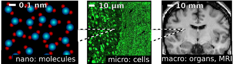
The three fundamental scales involved in MRI of biological samples. The molecular scale is of the order of 10⁻¹⁰ – 10⁻⁹ m. The characteristic correlation time of molecular motion is about 10⁻¹¹ – 10⁻¹² s. The cellular scale, or the scale of tissue microstructure, is of the order of 10⁻⁶–10⁻⁵m. The characteristic time scale of water diffusion over such distances is 10⁻³ – 10⁻¹ s. The macroscopic scale refers to structures that can be resolved using MRI, about 10⁻³ m for clinical or neuroscience applications. Apart from physiological motion, the intrinsic motion of water molecules is negligible on the macroscale.

As we discuss below, dephasing on the cellular scale brings in qualitatively new features as compared with the traditional NMR measurements in structureless solutions. Likewise, the cellular-scale structural complexity also affects NMR-measured diffusion (Tanner, 1979; Le Bihan et al., 1986; Basser et al., 1994; Callaghan, 1993; Jones, 2010), with the physics of diffusion and of transverse relaxation intimately intertwined, as the Brownian motion is the origin of the motional narrowing relevant at the MRI timescales.

From the methodological perspective, studying the cellular level tissue “microstructure” (Fig. 1) falls into the realm of meso-scopic physics, which is concerned with how the averaging over the structure at the mesoscopic, or intermediate scale (in between the atomic/molecular scale, and the macroscopic sample/voxel size) affects a macroscopic measurement, as reviewed recently (Novikov et al., 2016). The term “mesoscopic” is by definition relative. In our context, at the mesoscale, the molecular-level relaxation effects have already fully played out, yielding the local effective relaxation rates $R_1^{\text{mol}}$ (r) and $R_2^{\text{mol}}$ (r), which may further vary on the micrometer scale commensurate with cell dimensions. Signal acquisition over a macroscopic sample or an imaging voxel, much exceeding cellular dimensions, yields an extra averaging over the contributions having local relaxation rates and the locally varying Larmor frequency offset Ω(r) due to magnetic structure at the cellular level. In the absolute terms the cellular complexity at this micrometer scale gives rise to the term “tissue microstrucutre” (Jones, 2010); here we are concerned with the effects of magnetic tissue microstructure.

1.3. Outline and scope

The outline of this article is as follows. First, we consider a toy model of transverse relaxation (Sec. 2), in the spirit of Anderson and Weiss (1953). Although simple, it catches essential features of real processes and will serve as a reference point for further considerations. When presenting this model, we also introduce qualitative order-of-magnitude estimates for gaining insight in the physics of relaxation, which are used throughout this paper. We then qualitatively outline the essential signatures of transverse relaxation from the molecular, microscopic and macroscopic scales (Sec. 3), and present the phase diagram for the mesoscopic transverse relaxation, Fig. 6. In Sec. 4, introduce the mesoscopic Bloch-Torrey equation describing both diffusion and relaxation effects, and identify scaling relations based on the dimensionless variables. In Sec. 5, we consider technical details of the diffusion-narrowing and static dephasing regimes. Section 6 is devoted to the practically important case of relaxation in dilute suspensions of magnetic objects, where an additional small parameter, the low volume fraction of the suspension, enables further analytical treatment and the derivation of useful scaling laws. Section 7 introduces a more formal yet general treatment of mesoscopic relaxation, via the effective medium theory. In Sec. 8, we consider non-perturbative approaches aimed at exploring the crossover between the diffusion-narrowing and static dephasing regimes. Section 9 is devoted to applications of the discussed biophysical phenomena. Finally, in Sec. 10 we discuss common misconceptions, and in Sec. 11 we formulate the unresolved problems.

Figure 6:

Phase diagram of the mesoscopic transverse relaxation in the plane (α, t/τ_c). “SDR short times” refers to the condition $\delta \text{Ω}\cdot t\ll 1$. In the DNR, it is replaced by the less restrictive condition $t/{\tau }_c\ll 1$. Blue line shows the evolution of dephasing regime for a venous capillary orthogonal to the main field of 3 T with the typical parameters (dot) during the passage of a bolus of Gd-based contrast agent with the maximal concentration 10mM and the post-contrast concentration 1mM. The effect of increase in the vessel size is shown with light blue. Red circle shows a slightly smaller rodent capillary after an injection of 10 mgFe/kg. Small purple dot shows a hypothetical situation in which droplets with radius R = 1 μ m contain a Gd solution with the concentration 25mM (a 20-fold dilution of a typical manufactured solution). The purple dashed line shows the change in the relaxation regime, for a fixed measurement time t, when the droplet swells, keeping the same amount of contrast agent, diluting its concentration such that $\delta \text{Ω}\sim 1/{\mathit{R}}^3\sim {\tau }_c{}^{-3/2}$, yielding $\delta \text{Ω}\cdot {\tau }_c\sim {(t/{\tau }_c)}^{1/2}$.

From the outset, we would like to mention the limits of the scope of this review article. When discussing the physics of transverse relaxation, we focus on the simplest possible measurement scheme, which is the free induction decay. We do not analyze in detail various kinds of spin echoes. The spin echo is only discussed when it brings about a new physical essence, or when it helps us to draw contrast with the FID (cf. Sec. 3.4). Even less attention is paid to the contribution of multiple tissue compartments with different relaxation times. On top of the non-trivial relaxation physics (our main subject), this partial-contribution effect further complicates the interpretation of experimental data and, therefore, it deserves a dedicated approach, see the review article (Does, 2018) in the same journal issue.

2. A toy model of transverse NMR relaxation

2.1. Average over spins

Consider an ensemble of spins, each one exposed to a randomly varying magnetic field, B(t), of yet unspecified origin. We describe the transverse spin magnetization as a complex number, e^−iφ(t), where the phase¹

$$\phi (t)={\displaystyle {\int }_0^t\text{d}t\prime }\text{Ω}(t\prime ),\text{Ω}(t)=\gamma ({\rm B}(t)-B_0),$$ (1)

integrates the history of the magnetic field experienced by a given spin since the moment of excitation. Here Ω(t) is the instantaneous Larmor frequency relative to the nominal main field B₀ — i.e., it is the precession frequency in the rotating frame associated with an average spin, with γ the gyromagnetic ratio. The normalized signal from the whole spin ensemble is the average value of phase factors of individual spins:

$$S(t)=\langle e^{-i\phi (t)}\rangle \equiv p(\lambda )|{}_{\lambda =1}\cdot$$ (2)

The second identity in Eq. (2) tells that the signal is the Fourier transform, or the characteristic function

$$p(\lambda )=\langle e^{-i\lambda \phi }\rangle \equiv {\displaystyle \int \text{d}\phi 𝒫(\phi )}{e}^{-i\lambda \phi }$$ (3)

of the probability density function (PDF) 𝒫(φ) of all precession phases (1) accumulated by the time t, where 〈…〉 is the average with respect to 𝒫(φ). All of the richness of transverse relaxation effects originates from this averaging.

If different spins experience different yet static Larmor frequencies Ω, such that φ = Ωt, then the PDF 𝒫(φ) becomes equivalent (up to a trivial rescaling) to the PDF 𝒫(Ω) of the Larmor frequencies; the signal

$$S(t)={\displaystyle \int \text{d}}\text{Ω}𝒫(\text{Ω})e^{-i\text{Ω}t}\iff S(\omega )\equiv 𝒫(\omega ),$$ (4)

i.e. the spectral lineshape in the case of pure inhomogeneous broadening coincides with the PDF of Larmor frequencies in a sample (voxel).²

A less trivial situation occurs for the case of homogeneous broadening, where we assume that the random frequency Ω(t) for all spins has the same physical origin (i.e., is sampled from the same probability distribution 𝒫[Ω(t)] of functions). To average over the ensemble of these stochastic functions, e.g., Fig. 2, we Taylor-expand S(t), and average it term-by-term.

Figure 2:

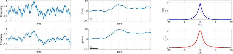
Left: Two random time series made from the same white Gaussian noise. The time courses have equal standard deviations and a four-fold difference in the correlation times, ${\tau }_c$ (black bars). Middle: The corresponding phases, Eq. (1). Right: The correlation function in the time (top) and frequency (bottom) domains. These functions are the same for both time courses up to the difference in the correlation times.

2.2. Cumulant expansion

Consider the case in which the typical spin phase is small, $\left|\phi \right|\ll 1$. We can then expand the signal in the Taylor series in φ and find its logarithm as

$$\ln S(t)=-i\langle \phi \rangle -\frac{1}{2}\left(\langle {\phi }^2\rangle -{\langle \phi \rangle }^2\right)+\dots .$$ (5)

The first term on the right-hand side is the mean phase over the ensemble of spins. The second term is proportional to the phase variance. Since the variance is always positive, this whole term is negative for any distribution of spin phases. The minus sign in front of this terms originates from i², which guarantees that this term describes signal attenuation. One can see that the expansion (5) is just the cumulant series (van Kampen, 1981; Kiselev, 2010) in the powers of λ for the characteristic function (3), taken at λ = 1. The cumulants generalize the relation between the variance and the second moment, 〈φ²〉: The nth-order cumulant is the nth-order moment with the subtracted reducible contributions from all the lower orders. While averaging the expanded exponential gives all moments as coefficients, the logarithm of this series has the same form, but with the moments replaced by the cumulants, cf. (Kiselev, 2010) for a detailed discussion.

Let us express the phase via the instantaneous Larmor frequency using Eq. (1). For stationary systems, that do not change their properties during the measurements, the first term in Eq. (5) takes the form

$$\langle \phi \rangle =\langle \text{Ω}\rangle t.$$ (6)

This term describes the signal phase accumulation with the constant rate 〈Ω〉. While this rate can be the goal of a measurement (e.g., in the quantitative susceptibility mapping), it is effectively removed by working with the signal magnitude or, if constant across an MR image, can be set to zero by tuning the resonance frequency of the scanner. In what follows, we focus on the signal relaxation described by the second term in Eq. (5), from now on assuming 〈Ω〉 ≡ 0 without the loss of generality:

$$\ln S(t)=-\frac{1}{2}{\displaystyle {\int }_0^t\text{d}}{t}_1\text{d}{t}_2\langle \text{Ω}(t_1)\text{Ω}(t_2)\rangle +\dots ,$$ (7)

where the integration over both time variables is performed from 0 to t as in Eq. (1). To obtain this expression, we substituted the phase in Eq. (5) from Eq. (1), represented the square of the resulted time integral as a double integral over independent variables t₁ and t₂, and subsequently applied the averaging with account for 〈Ω〉 = 0.

2.3. Cumulants as correlation functions

Let us now focus on the leading ∼ Ω² term, Eq. (7), to develop physical intuition, which will then help us consider qualitatively the role of the higher-order terms. The averaged quantity in the integral in Eq. (7) is the correlation function of the instantaneous Larmor frequency, Fig. 2.³ For stationary systems, this function is time translation-invariant, i.e., it depends only on the time interval, Fig. 3:

$$J(t_2-t_1)=\langle \text{Ω}(t_1)\text{Ω}(t_2)\rangle$$ (8)

and is an even function of this interval, J(‒τ) = J(τ). This correlation function can be roughly characterized by two parameters, which are the variance of Ω(t),

$$J(\tau )|{}_{\tau =0}=\langle {\text{Ω}}^2\rangle$$ (9)

and the correlation time τ_c, which shows at which interval τ the value Ω(t + τ) becomes statistically independent from Ω(t), see the left panel of Fig. 2 for an illustration. In other words, τ_c is the scale over which J(t) is non-negligible, i.e. it shows the extent of memory about the temporal evolution of Ω(t).

Figure 3:

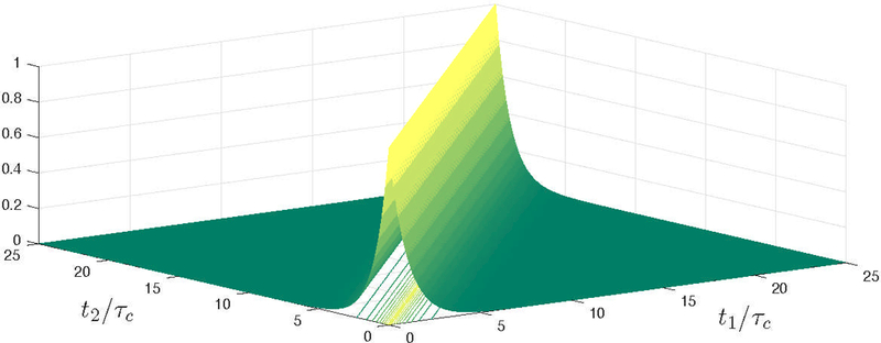
An example of a correlation function, Eq. (8), shown as a surface with contour lines projected on the integration plane (t₁, t₂) in the integral in Eq. (7).

In general, the double integral in Eq. (7) depends on the precise shape of the function (8). However, it simplifies in the two important limiting cases, of short and long times.

For short times, t ≪ τ_c, the correlation function does not change significantly within the integration area, being well approximated by its value at t = 0. This constant can be factorized out of the integral leaving the remaining integration trivial,

$$\ln S\simeq -\frac{1}{2}\langle {\text{Ω}}^2\rangle t^2,t\ll {\tau }_c.$$ (10)

Note that this result is simple and completely general: irrespective of the distribution of Ω(t), the short-time limit reduces the problem to that of the inhomogeneous broadening, Eq. (4), since for each spin its frequency can be considered constant — as long as the accumulated phases remain small. To the leading order in t, the signal is determined by the second cumulant of 𝒫(Ω) — the PDF of all values of Ω in the time series (i.e., involving a function 𝒫(Ω), not a functional 𝒫[Ω(t)]).

For long times, t ≫ τ_c, the integral in Eq. (7) is mainly contributed by the diagonal, t₁ ≈ t₂, since the correlation function tends to zero for large time separations (Fig. 3). Time translation invariance suggests a natural change of variables: t₁, t₂ → t ≡ t₁, τ ≡ t₂ − t₁. When J(τ) decays faster than 1/τ, we can integrate the correlation function over its cross-section first (Fig. 3), extending the integration to all τ, to obtain the signal in the form

$$\ln S_t{}_{\gg {\tau }_c}\simeq -R_{2}t,R_2=\frac{1}{2}{\displaystyle {\int }_{-\infty }^{\infty }d}\tau J(\tau ),$$ (11)

where we used the common notation for the transverse relaxation rate R₂. Its magnitude can be estimated as the product of the height of the integrand, Eq. (9), with the width, τ_c; this gives R₂ ∼ 〈Ω²〉 τ_c. Note, again, a drastic reduction in the number of relevant parameters that determine R₂ in the limit t → ∞: While the precise shape of the correlation function is defined in principle by an infinite number of parameters, it is a single number, the integral of this function, that defines R₂. This is an example illustrating the notion of relevant degrees of freedom in physics: The details of fast dynamics on a fine scale (for times of the order of τ_c in the present example) are coarse-grained, and most of them become irrelevant on a coarser scale (time t ≫ τ_c) — with an exception of just a few parameters (a single relevant one, R₂, in the present example).

The integral in Eq. (7) is often considered in terms of the Fourier transformed correlation function, J(ω),

$$\ln S(t)=-2{\displaystyle \int \frac{\text{d}\omega }{2\pi }}\frac{{\sin }^2(\omega t/2)}{{\omega }^2}J(\omega ).$$ (12)

Here the sinc function appears as the Fourier transform of the measurement interval 0 < t_1,2 < t when performing a continuous Fourier transformation on the whole time axis. It is straight forward to recover the short-time asymptotic form, Eq. (10), by taking the limit ωt ≪ 1 in this integral. The long-time asymptotic form, Eq. (11) is obtained by noticing that the factor sin(ωt/2)/ω approaches πδ(ω) for long times, which gives R₂ = J(ω)|_ω=0/2 in agreement with Eq. (11).

Since the above consideration was based on the expansion for small phases, Eq. (5), it might appear that the result, Eq. (11), can be questioned for strongly attenuated signals for which R₂t ≫ 1. We now find the validity criterion for Eq. (11) by considering the correction terms to Eq. (5). The third-order terms include 〈φ³〉, 〈φ²〉〈φ〉, 〈φ〉³; the higher-order terms include all possible ways of averaging the higher powers of φ forming the cumulant expansion as already mentioned above. Substitution of Eq. (1) results in the cumulant expansion for ln S with the first nonvanishing term written in Eq. (7) and with the nth-order term

$$\frac{{(-i)}^n}{n!}{\displaystyle {\int }_0^t\text{d}}{t}_1\dots \text{d}{t}_n{\langle \text{Ω}(t_1)\dots \text{Ω}(t_n)\rangle }_c,$$ (13)

where the subscript ‘c’ stands for “cumulant”. The cumulants are called also the reduced correlation functions because they turn to zero when any of averaged quantities, Ω(t_m) is uncor related with another (van Kampen, 1981). This means that the cumulants turn to zero when the separation between any of two time points exceeds the correlation time, τ_c. Another important property follows from the time translation invariance, which means that no property of the considered system changes if our experiment is repeated at a different time. Equivalently, shift ing all time variables by the same amount, t_m → t_m + ∆t, does not change any cumulant. Summarizing these properties, the general term, Eq. (13), can be estimated as ∼ δΩⁿ τ_cⁿ⁻¹t, where δΩ denotes the typical value of Ω, which is of the order of its standard deviation $\sqrt{\langle {\text{Ω}}^2\rangle }$ (as Ω(t) has zero mean). This yields that the relaxation in the t ≫ τ_c limit will become asymptotically monoexponential: S ∼ e^−R₂t, where the rate R₂ acquires contributions from all higher-order cumulants. This means that the first equality in Eq. (11) remains valid, while the value of R₂ changes.

To control the cumulant series convergence, it is convenient to introduce the dimensionless parameter

$$\alpha =\delta \text{Ω}\cdot {\tau }_c,\delta \text{Ω}=\sqrt{\langle {\text{Ω}}^2\rangle ,}$$ (14)

which is a typical value of the precession phase accumulated over the correlation time τ_c. In terms of this parameter, the nth order term (13) is ∼ αⁿ · t/τ_c. Hence, each subsequent term becomes less important, and truncating Eq. (5) already at the second-order term is justified, when

$$\alpha \ll 1.$$ (15)

Under this “perturbation theory” condition, Eq. (11) is valid irrespective of long t.

Note that the time translation invariance and the separation of scales t ≫ τ_c (i.e., having a finite correlation time) allows us to effectively factor out the overall (long) time t from each term (13), and yields a substantially improved condition, δΩ·τ_c ≪ 1, for the convergence of the cumulant expansion (5). Naively, in that series, each power of φ should contribute φ ∼ δΩ · t, and hence, one would think that the series should converge only when δΩ ⋅ t ≪ 1, — a condition that becomes invalid for sufficiently long t.

The observation that the overall t can be factored out from each term of the cumulant series, such that the overall relaxation becomes monoexponential in the limit t ≫ τ_c can be understood from a different angle.

2.4. Relaxation at long times as the Central limit theorem

Consider the random phase in Eq. (1). There, the integrand Ω(t) is correlated over the time intervals of typical duration τ_c. This means that an individual spin phase in the long-time limit can be approximated by a sum of N ∼ t/τ_c ≫ 1 statistically independent contributions, $\phi ~{\displaystyle {\sum }_{n=1}^N{\phi }_n}$, where each φ_n ∼ α can be treated as an independent random variable. When the number N of independent contributions to the random variable φ becomes large, the Central limit theorem (CLT) tells that its characteristic function (3) approaches that of the Gaussian distribution, $p(\lambda )\simeq e^{-i\lambda \langle \phi \rangle -{\lambda }^2{\langle {\phi }^2\rangle }_c/2}$, with the higher-order cumulants being less relevant. Moreover, according to the CLT, the mean values and variances from the independent contributions add up, i.e. $\langle \phi \rangle \equiv 0$, and ${\langle {\phi }^2\rangle }_c\sim N{\sigma }_c^2$, where ${\sigma }_c^2\equiv \langle {\phi }_n^2\rangle$ is the variance for each independent contribution. We again obtain the monoexponential relaxation with the rate $R_2\text{}~\text{}{\sigma }_c^2/{\tau }_c$.

In general, the rate ${\sigma }_c^2\tau c$ is an unknown function of α, and depends on the form of all the cumulants. However, for weak dephasing (15), dropping all the higher-order terms leads to ${\sigma }_c^2~{\alpha }^2$ and

$$R_2\sim {\alpha }^2/{\tau }_c=\langle {\text{Ω}}^2\rangle {\tau }_c,$$ (16)

as it was already found after Eq. (11)

To sum up, monoexponential signal relaxation for long times, $t\gg {\tau }_c$, follows from the Central limit theorem, describing the random walk of the precession phase (1). The phenomenon of lineshape narrowing is reflected in the τ_c-dependence of the rate (16): the shorter τ_c, at a fixed variance $\langle {\text{Ω}}^2\rangle$ of the random Ω(t), the more effective is the averaging, and the smaller the rate. Such narrowing due to dipolar couplings has been first considered by Bloembergen et al. (1948) and by Anderson and Weiss (1953). In the biophysical context, as we will describe below, this effect occurs due to the motion of spins sampling Ω(r(t)) on a trajectory, e.g., on a Brownian path. A similar effect of the dephasing of an electron spin phase due to scattering off multiple impurities in the presence of spin-orbit interaction is known as the Dyakonov-Perel relaxation (Dyakonov and Perel, 1971).

3. Relaxation from the three scales

In this Section, we go over main qualitative features of the contributions to the overall relaxation from the three distinct scales of Fig. 1, from the smallest to the largest.

3.1. Molecular scale

Signal relaxation on the molecular scale is always present as a background for all other relaxation processes. We briefly address both the transverse and the longitudinal relaxations, since the latter will serve for comparison in a few examples discussed below. While the existence of spin is a pure quantum effect, we do not need quantum mechanics for the present simplified consideration that follows the discussion by Goldman (2000). It is sufficient to know that a spin flip in the quantum language or, equivalently, tilting a spin in the classical language, is a resonant process, giving name to NMR.

Consider first the transverse relaxation. The above toy model instantiated via a very fast molecular motion, where the stochastic magnetic field appears, for example, as the dipole-dipole interaction of two proton spins in water molecules. The magnetic field is changing due to random molecular rotation, since the dipole field is direction-dependent. The molecular motion is very fast, with the typical time τ_c ∼ 1 ps = 10⁻¹² s. This means that our measurements performed on the millisecond MRI time scale always fall in the regime of very long times, t ⋙ τ_c. In this regime, transverse relaxation rate is determined by J(ω)|_ω=0 [recall the discussion after Eq. (12)], which can be understood also from the quantum-mechanical point of view: Transverse relaxation is a process of dephasing; changing the spin precession phase does not change its energy, thus the quantum transition is sensitive to the perturbation components at $ħ\omega =0$.

In contrast, the longitudinal relaxation is associated with changing the energy of spins in the external magnetic field. The corresponding frequency is the Larmor frequency Ω_L. As NMR is a resonant process, a fluctuating magnetic field causes longitudinal relaxation most efficiently when its characteristic frequency 1/τ_c ∼ Ω_L. Proper calculations support this qualitative conclusion by revealing the proportionality R₁ ∼ J(ω)|_ω=ΩL (in this discussion, we refer to frequency in the laboratory frame).

At this stage we can recover the well-known result about different dependence of both relaxation rates on the rate of molecular motion (Bloembergen et al., 1948; Goldman, 2000). Consider for example a water molecule in which the magnitude of spin-spin interaction of two protons is constant, but the correlation time τ_c depends on the environment, for example if the molecule is free, or if it sticks to a slowly moving protein. In terms of the above model, this constant interaction amplitude squared ∼ J(t)|_t=0 is translated into a constant variance of the random field, Eq. (9). In the spectral domain, this constant maps on the constant integral of J(ω),

$$\langle {\text{Ω}}^2\rangle ={\displaystyle \int \frac{\text{d}\omega }{2\pi }}J(\omega )=\mathrm{const.}$$ (17)

This means that the area under J(ω) is conserved, while the width of J(ω) changes as 1/τ_c. This result in different patterns for the dependence of R₁ and R₂ on the “tumbling rate” 1/τ_c, as illustrated in Fig. 4. The simplest single time-scale form for J(ω) convenient to have in mind is a Lorentzian

$$J(\omega )=\frac{2\langle {\text{Ω}}^2\rangle {\tau }_c}{1+{(\omega {\tau }_c)}^2}\iff J(t)=\langle {\text{Ω}}^2\rangle e^{-\left|t\right|/{\tau }_c},$$ (18)

which is correctly normalized in the view of Eq. (17). Realistic J(ω) from the Bloembergen-Purcell-Pound theory (BPP) is more complicated (Bloembergen et al., 1948), but not qualitatively different from Eq. (18), cf. right panel of Fig. 4. The exponentially-decaying correlations in the time domain, of the kind in Eq. (18), is a natural assumption when having a single well-defined time scale for the underlying stochastic process.

Figure 4: Molecular relaxation.

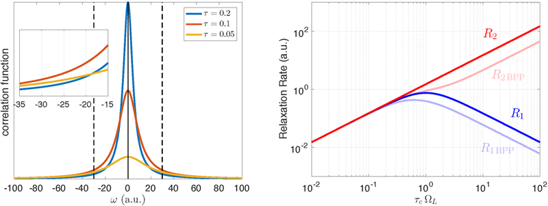
Left: The function J(ω) for three different correlation times, illustrated via Eq. (18). The width of J(ω) is estimated as $1/{\tau }_c$. From the conservation of area under the curve J(ω), it follows that the height $J(\omega ){|}_{\omega =0}$ of the function scales as ${\tau }_c$, which explains the increase in R₂ with ${\tau }_c$. Since the value of R₁ is defined by $J({\text{Ω}}_L)$ (which is shown with the dashed vertical lines), it has a maximum at ${\tau }_c\sim 1/{\text{Ω}}_L$. Inset: The value $J({\text{Ω}}_L)$ is small when the spectral power is spread too much (too small ${\tau }_c$) and when it is concentrated near zero (too long ${\tau }_c$). Right: The corresponding behavior of R₁ and R₂ as function of ${\tau }_c$, i.e. for the increasingly slow molecular motion at fixed ${\text{Ω}}_L$. The actual relaxation rates for water protons in the BPP calculation (Bloembergen et al., 1948) are slightly different due to the presence of two spins (pale colors).

Under the normal conditions, water molecules move very fast in comparison with the proton Larmor frequency Ω_L/2π ∼ 10⁸ Hz at the typical field strength of a few Tesla. It is well known that both relaxation rates increase in solutions of large molecules such as proteins. Further slowing down of water motion results in the decoupling of relaxation rates: R₁ ∼ J(Ω_L) starts decreasing, while R₂ keeps increasing (Fig. 4), such that, for the simplest model J(ω) from Eq. (18), R₁ ∼ R₂/[1+(Ω_Lτ_c)²]. This results in a principal difference in the R₁ and R₂ effects of contrast agents.

In particular, the R₁ effect is local for all practical purposes of biological MRI. To understand this, let us estimate how far its effect on R₁ and R₂ can reach from a strongly magnetized particle of a contrast agent. Consider water molecules a distance ℓ from this particle. In time t, these molecules move over the distance of the order of $\sqrt{Dt}$ due to a diffusive motion with diffusion constant D. In order to experience an essential change in the dipole field, this motion should result in an angle $\sqrt{Dt}/\ell \sim 1$ at which the molecules are seen from the particle. In other words, the characteristic frequency ω ∼ 1/t of magnetic field variations experienced by a moving molecule should scale as $D/{\ell }^2$. Longitudinal relaxation is the most efficient when this rate is comparable with the Larmor frequency, $D/{\ell }^2\sim {\Omega }_L$. Using the typical values D ∼ 1 µm²/ms and Ω_L ∼ 10⁹ s⁻¹, we obtain an estimate $\ell \sim 1\text{\hspace{0.17em}nm}$ for the optimal “interaction distance” with the contrast agent. This distance is negligible compared to the scale of cells in biological tissues, which are of the order of a micrometer or greater.

Conversely, the transverse relaxation is most efficient as $\omega \to 0$, i.e., when the rate D/ℓ² tends to zero, which implies ℓ → ∞. This means that the R₂ effect can spread far outside the physical location of a contrast agent, which will be considered in detail below. As a side note, the selective effectiveness of longitudinal relaxation results in a complicated dependence of the contrast agent relaxivity on the main magnetic field (Gillis and Koenig, 1987).

3.2. Microstructural (cellular) scale

We now proceed with the main subject of this review, which is transverse relaxation in biological tissues. We focus on relaxation of water protons due to its abundance in tissues and its role in MRI, rather than due to any special physical properties.

3.2.1. Chemical and susceptibility effects

There are two sources of enhanced transverse relaxation in biological tissues as compared with that in the pure water. They can be classified according to the spatiotemporal scale on which dephasing takes place.

The first one is the presence of diverse solutes with large molecules that can bind water and thus accelerate relaxation as discussed above in Sec. 3.1. This effect depends on the local chemical composition inside a biological compartment such as as specific cell species. The effect is strong: The relaxation time is reduced from about 2s in pure water (R₂ ≈ 0.5s⁻¹) to values below 100 ms (R₂ ∼ 10s⁻¹). This is essentially a molecular effect, falling under the realm of the previous Sec. 3.1.

The second one is a mesoscopic effect due to a higher concentration of a paramagnetic substance in a specific tissue compartment (for example, in the blood pool or in iron-loaded cells). Such local magnetic susceptibility, spatially varying on the scale of tissue microstructure, induces an additional magnetic field when exposed to the strong main field B₀ of an MRI scanner. The induced field dephases spins not only within the compartment, but also in the adjacent regions, thus extending the effect of paramagnetic substance outside the volume where it is physically present. Typically, the induced magnetic field spans over distances ℓ_c commensurate with the dimensions of paramagnetic compartment, i.e., micrometers or tens of micrometers. The corresponding correlation time of magnetic field fluctuations experiences by water protons, due to the diffusive motion of the spin-carrying molecules, is in the range of τ_c ∼ ℓ_c²/D ∼ 1−100 ms, which is comparable to the typical time available for MR measurements after a spin excitation (more details Sec. 5 below). This results in a particular richness of the mesoscopic relaxation physics, and its nontrivial relation to the magnetic tissue microstructure. Understanding the mechanisms of the transverse relaxation on the micrometer scale is desirable as an instrument for probing the microstructure and function of biological tissues in vivo.

3.2.2. The time-dependent relaxation rate

All the essential signatures of the mesoscopic relaxation originate from the physics of averaging in Eq. (2). The above estimates suggest that the relaxation is not expected to be monoexponential — in fact, the most important qualitative feature of the mesoscopic transverse relaxation is being in the transient regime, Fig. 5, with the monoexponential relaxation approached only asymptotically, at t → ∞ (which practically may mean never, depending on the length scales associated with tissue heterogeneities). The signal is characterized by a time-dependent relaxation rate R₂(t), both for the FID, and, generally, for any sequence with finite refocussing intervals. A natural definition for the “instantaneous” time-dependent relaxation rate is

$$R_2(t)\equiv -\frac{\text{d}}{\text{d}t}\ln S={\displaystyle {\int }_0^t\text{d}t}\prime J(t\prime )+\dots ,$$ (19)

where the first term follows from Eq. (7), while “…” corresponds to contributions from the higher-order cumulants.

Figure 5: Mesoscopic relaxation.

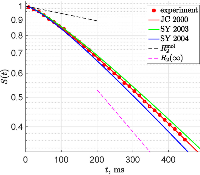
Normalized gradient echo (FID) signal (red dots) in a semilog scale from a suspension of paramagnetic beads of about 20 $\mu m$ in diameter, in water with added gelatin, from (Storey et al., 2015), exhibits a characteristically slow crossover behavior, interpolating between the initial “molecular” relaxation and the $t\to \infty$ monoexponential decay. Red line shows a fit by Eq. (25) based on the correlation function proposed by Jensen and Chandra (2000b) (JC 2000). The two dashed lines correspond to $e^{-{\mathit{R}}_2^{\text{mol}}t}$ and $e^{-{\mathit{R}}_2(\infty )t}$ , with R₂(∞) given by Eq. (27). The slope R₂(t) of the signal barely reaches the long-time limit R₂(∞) even at fairly long echo trains. Also shown are the two more realistic models, for permeable spheres (Jensen and Chandra, 2000b; Kiselev and Novikov, 2002; Sukstanskii and Yablonskiy, 2003) (SY 2003), and for impermeable spheres (Sukstanskii and Yablonskiy, 2004) (SY 2004), green/blue, for the same fit parameters as estimated from JC 2000, Eq. (25). It is quite easy to make these models fit the experimental points equally well; studying the relative accuracy and precision of these models is a subject of on-going investigation. Here, we plot these three theoretical curves to emphasize their qualitative and quantitative similarity (see discussion in text).

Here, we give an overall qualitative picture for the behavior of S (t) and R₂(t), and consider inhomogeneous and homogeneous broadening cases separately. We will discuss the FID signal only, with more precise calculations and other measurement sequences considered in the subsequent sections.

3.2.3. Inhomogeneous broadening: SDR

The inhomogeneous broadening, or the static dephasing regime (SDR), can be viewed via the lineshape (4) as a distribution of frequencies 𝒫(Ω) specifically originating from the susceptibility-induced field (Yablonskiy and Haacke, 1994; Kiselev and Posse, 1999; Jensen and Chandra, 2000c). We consider this situation in detail below in Sec. 5.4 in general, and in Sec. 6.2 for a well15 studied case of dilute suspensions of magnetic inclusions.

The SDR contribution behaves as ln S ∼ −t² and R₂ ∼ t at short times, in agreement with the general result (10). Here, the distinction between short and long times is made by δΩ · t ≪ 1 and δΩ · t ≫ 1 correspondingly, as there is no other time scale in the problem (such as the correlation time τ_c to give the effect of “forgetting” the memory about the phase history).

Absent τ_c, the relaxation at long times can take different functional forms. When monoexponential, it is not the consequence of the CLT, Sec. 2.4, and it can be considered accidental — actually, having to do with the 1/r^d scaling of the dipole field in d dimensions, that is being convolved with the susceptibility sources, cf. Sec. 6.2 below.

In the pure SDR (no diffusion), spin echo experiment eliminates the inhomogeneous line broadening, and yields the molecular R₂ relaxation. The nontrivial mesoscopic correction to spin echo emerges due to diffusion, cf. Sec. 5.4 and 6.2.

3.2.4. Homogeneous broadening: DNR

The homogeneous broadening regime, or the diffusion narrowing regime (DNR), and any intermediate regime where the diffusion cannot be discarded, is nontrivial in the following sense: The averaging 〈…〉 in Eq. (2) should be effectively performed over the Brownian paths r(t), giving rise to the stochastic contributions Ω(t) ≡ Ω(r(t)) for the phase of each spin. Ultimately, this means that the signal becomes sensitive to the spatial correlations of magnetic structure (embodied by the correlation functions of Ω(r), or of the underlying susceptibility χ(r)), probed by the diffusing spins. Establishing the relation between the spatial structure correlation functions and the temporal ones (that can be measured) is the fundamental problem in this regime.

To the lowest (i.e., second) order in Ω(r), this relation was obtained by Jensen and Chandra (2000b) who showed that the temporal correlation function

$$J(t_1-t_2)={\langle \text{Ω}(\mathbf{\text{r}}(t_1))\text{Ω}(\mathbf{r}(t_2))\rangle }_{\text{medium; paths}}={\langle {\Gamma }_{\text{Ω}}(\mathbf{r}(t_1)-\mathbf{r}(t_2))\rangle }_{\text{paths}}$$ (20)

is given by the average over the Brownian paths r(t) of the twopoint spatial correlation function

$${\Gamma }_{\text{Ω}}(\mathbf{r})=\frac{1}{V}{\displaystyle \int \text{d}{\mathbf{r}}_0}\text{Ω}({\mathbf{r}}_0+\mathbf{r})\text{Ω}({\mathbf{r}}_0)$$ (21)

of the local Larmor frequency variation Ω(r). The details about averaging over the paths will be explained below, in Sections 4 and 5 — see, in particular, Eq. (50) in Sec. 5.3. The correlation function (20) can be measured using asymmetric spin echo (Jensen et al., 2006).

To give an idea of the qualitative features of the mesoscopic signal, Fig. 5, it is convenient to have a tractable yet sufficiently general model. According to the relation (20), a model for the signal described within the Gaussian phase approximation (GPA) (i.e., to the order $\langle {\phi }^2\rangle$), is set by the corresponding model for the random medium to the second order in Ω(r), via a single correlation function (21). A convenient ansatz for Eq. (21) was suggested by Jensen and Chandra (2000b):

$${\Gamma }_{\text{Ω}}(\mathbf{r})=\langle {\text{Ω}}^2\rangle e^{-{(r/2{\ell }_c)}^2}\iff {\Gamma }_{\text{Ω}}(\mathbf{q})={(4\pi )}^{3/2}\langle {\text{Ω}}^2\rangle {\ell }_c{}^3{e}^{-q^2{\ell }_c{}^2}$$ (22)

where ℓ_c is the correlation length. Average over the Brownian paths, Eq. (50), leads to the temporal correlation function (20) of the form

$$J(t)=\frac{\langle {\text{Ω}}^2\rangle }{{(1+t/{\tau }_c)}^{3/2}},{\tau }_c=\frac{{\ell }_c{}^2}{\mathit{\text{D}}}$$ (23)

where τ_c is the diffusion time over the correlation length of the medium (tissue). Neglecting the higher-order terms in Eq. (19), this function completely determines the signal (7). Performing the two subsequent integrations, one obtains the relaxation rate

$$R_2(t)=R_2^{\text{mol}}+R_2^{\text{meso}},R_2^{\text{meso}}=\frac{2{\alpha }^2}{{\tau }_c}\left(1-\frac{1}{\sqrt{1+t/{\tau }_c}}\right),$$ (24)

and the FID signal

$$\ln S=-R_2^{\text{mol}}t-2{\alpha }^2\left(\frac{t}{{\tau }_c}-2\sqrt{1+\frac{t}{{\tau }_c}}+2\right).$$ (25)

Here, we added the constant molecular rate $R_2^{\text{mol}}$ inherent to all the NMR measurements, Sec. 3.1, providing a “background” on which the mesoscopic relaxation evolves. The signal (25) describes the FID measurement in a random bead suspension quite well, Fig. 5. For the corresponding spin echo expression, see (Storey et al., 2015).

We note that averaging over the Brownian paths in Eq. (20) results in a qualitatively distinct functional form of the correlation function (8), making it decay algebraically, Eq. (23), rather than exponentially, as in BPP molecular model or in the theory of Anderson and Weiss (1953), cf. Eq. (18). The same qualitative changes should occur for all higher-order correlation functions entering Eq. (13), although no one dared to show that consistently and rigorously yet. In Sec. 8, we review selfconsistent attempts to go beyond the second order of the perturbation theory, to extend the DNR results onto the parameter domain α ∼ 1, effectively interpolating between the DNR and SDR.

Historically, DNR was first developed (Gillis and Koenig, 1987; Kiselev and Posse, 1998; Jensen and Chandra, 2000b; Kiselev and Novikov, 2002; Sukstanskii and Yablonskiy, 2003,2004) for dilute suspensions of magnetic objects of particular shape to the second order in Ω(r), as reviewed in detail Sec. 6 below, and by Dickson et al. (2011). All these results can be reexpressed via the general relation (20) with a suitable cor relation function; for the dilute suspensions, such a function scales in proportion to the volume fraction ζ of the objects, cf. Sec. 6.1 below.

3.2.5. Transient character of the mesoscopic signal

Figure 5 shows a qualitatively general behavior of the FID signal in the DNR. We can see that the numerical differences between the simple model (25), and more involved models of Jensen and Chandra (2000b); Kiselev and Novikov (2002); Sukstanskii and Yablonskiy (2003), and Sukstanskii and Yablonskiy (2004) for the dilute suspension of permeable and of impermeable spheres, respectively, are relatively minor, and relate to the presence of sharp boundaries for the field and for the diffusion. (These differences become more pronounced for the spin echo.) However, here we specifically plot all three models for the same set of parameters, to emphasize their qualitative and quantitative similarities, which are as follows:

1. The slope (19) is always increasing with t, from the initial

   $$R_2^{\text{mol}}\equiv R_2(t){|}_{t\to 0}$$ (26)

   to its long-time limit

   $$R_2(\infty )=R_2^{\text{mol}}+R_2^{\text{meso}}(\infty ),$$ (27)

   where $R_2^{\text{meso}}(\infty )=2{\alpha }^2/{\tau }_c$ for the model (24), having the expected scaling with α and τ_c, cf. Sec. 2.4.

2. The time scale on which the switching between the rates (26) and (27) occurs is t ∼ τ_c. Using biophysical modeling (Kiselev and Posse, 1998; Jensen and Chandra, 2000b; Kiselev and Novikov, 2002; Sukstanskii and Yablonskiy, 2003, 2004; Jensen et al., 2006; Novikov and Kiselev, 2008), one can determine the characteristic length scale of the spatial distribution of the magnetic microstructure and its variance $\langle {\text{Ω}}^2\rangle$ characterizing magnetic heterogeneity (e.g., the amount of paramagnetic ions at the mesoscale).

3. The approach of the rate (24) to its long-time limit (27) is very slow, in this case as ∼ t^−1/2, which is a consequence of the slow power-law decay (23) of the corresponding correlation function — a consequence of the gradual coarse-graining (Novikov et al., 2016) of the random medium via the increasing diffusion length. Very similar power-law tails occur in the instantaneous diffusion coefficient (Novikov et al., 2014), emphasizing the similarities between the mesoscopic description of diffusion and relaxation. Note that the correlation function of the form (18) decays qualitatively faster (Kennan et al., 1994; Novikov and Kiselev, 2008; Ruh et al., 2015), which is a good description for a more ordered (e.g., periodic or hyperuiniform) medium, but turns out to be less applicable for the more realistic short-range spatial correlations in the random magnetic structure.

3.3. Macroscopic scale

Relaxation on the macroscopic scale is caused by the inhomogeneities of the main magnetic field that are of the order or larger than sample size or an imaging voxel. As an example, they can be created by overall non-spherical sample shape in NMR experiments, or poor shimming in MRI, e.g., near the sinuses in the brain. Molecular motion can be fully neglected on this scale. According to the above considerations, it is only the transverse relaxation that is affected by such inhomogeneities; it is always in the short-time, SDR limit, with the expansion in t starting from ln S ^macro ∼ −t², cf. Eq. (10), such that the corresponding $R_2^{\text{macro}}\sim t$ as t → 0. The explicit shape of the signal can be obtained knowing the slice profile, e.g. a sinc-function for a rectangular slice (Yablonskiy, 1998). Since the molecular motion is negligible on the macroscopic scale, any kind of spin echo completely removes the macroscopic dephasing.

3.4. The net relaxation from all scales

The above consideration demonstrates that the classic NMR equation for the FID relaxation rate,

$$R_2^{*}=R_2+R_2^{\prime },$$ (28)

becomes misleading in the context of biological tissues that have mesoscopic signal contributions. The original meaning of the two terms in Eq. (28) are as follows: the molecular $R_2=R_2^{\text{mol}}$, and the macroscopic part $R_2^{\prime }=R_2^{\text{macro}}$ that is completely refocussed by using any kind of spin echo.

Brownian motion of spin-carrying molecules fundamentally prevents full refocussing of the mesoscopic effects at any finite echo time. In fact, when the echo time exceeds τ_c, the relaxation rate for the spin echo, CPMG, and any other sequence with refocusing will approach that for the FID, while for short echo times a larger portion of signal can be refocused (Kennan et al., 1994; Kiselev and Posse, 1998; Jensen and Chandra, 2000b; Kiselev and Novikov, 2002; Sukstanskii and Yablonskiy, 2003, 2004).

In the framework of MRI in biological tissues, Eq. (28) should be replaced with the contribution of all three involved spatiotemporal scales shown in Fig. 1:

$$R_{2\text{GE}}(t)=R_2^{\text{mol}}+R_2^{\text{meso}}(t)+R_2^{\text{macro}}(t),$$ (29)

$$R_{2\text{SE}}(t)=R_2^{\text{mol}}+R_{2\text{SE}}^{\text{meso}}(t),$$ (30)

for the gradient echo (FID) and spin echo, correspondingly. Note that the mesoscopic effects contribute differently in the GE and SE rates, so that, generally, $R_{2\text{SE}}^{\text{meso}}(t)\le R_2^{\text{meso}}(t),$ and their equality occurs only at t → ∞. The addition of the rates is a general consequence of kinetic theory (Lifshitz and Pitaevskii, 1981), where the contributions from different sources in the collision integral do not interfere to the lowest order; in our case, the cross-correlation terms $\langle {\text{Ω}}^{\text{mol}}(t_1){\text{Ω}}^{\text{meso}}(t_2)\dots {\text{Ω}}^{\text{macro}}(t_n)\rangle$ vanish because of significantly distinct and independent spatio-temporal statistics of these contributions.

3.5. How to separate molecular and mesoscopic effects?

Let us address a practically important question: how can we ensure that we measure only the genuine molecular rate, $R_2^{\mathrm{mol}}$, without the mesoscopic effects? This could be useful for separating distinct biophysical contributions to the signal — e.g., magnetic ions distributed uniformly and affecting $R_2^{\text{mol}}$, versus the cellular-scale susceptibility variations affecting $R_2^{\text{meso}}$(t). A model-free way to separate between these contributions would help understand which one is a better marker of a given pathology. Besides, this would ensure reproducibility between different sites and vendors, where currently different degrees of admixture of the mesoscopic contribution occur due to different echo timings in a variety of spin-echo measurement sequences.

Using the shortest possible echo times is an obvious possibility, with a number of sequences available. However, even the shortest realistic SE or CPMG echo times, of a few ms on clinical systems, generally still yield an admixture of the mesoscopic contributions. Can one obtain pure $R_2^{\text{mol}}$ without applying refocussing pulses, thereby also avoiding hardware issues with B₁ inhomogeneities and specific absorption rate?.

The simple and universal answer that we are advocating in this article is rooted in the fundamental quadratic-in-time SDR limit (10) of any mesoscopic or macroscopic contribution to the signal at short times, or, equivalently, linearly vanishing $R_2^{\text{meso}}(t)$ and $R_2^{\text{macro}}(t)$ as t → 0. It is only $R_2^{\text{mol}}$ that does not vanish (here we of course realize that t → 0 is not taken literally; t ∼ 1 ps, at which $R_2^{\text{mol}}$ may vanish as well, is unattainable.) Therefore, $R_2^{\text{mol}}$ should be determined from a simple FID/GE measurement by taking the slope of ln S at t → 0,

$$R_2^{\text{mol}}\equiv -\frac{\text{d}\text{ln}S}{\text{d}t}{|}_{t\to 0}\cdot$$ (31)

This slope can be practically calculated, e.g., by a poloynomial approximation of the FID signal near t = 0, cf. black dashed line in Fig. 5. The operational definition (31) is in complete analogy with the way the diffusion coefficient is determined as the slope of lnS with respect to the b-value in the b → 0 limit.⁴ Defined in this way, the genuine $R_2^{\text{mol}}$ can in principle be made reproducible, and the mesoscopic and molecular effects can be studied separately from each other.

3.6. Phase diagram for the mesoscopic relaxation

Figure 6 qualitatively summarizes the regimes of the mesoscopic transverse relaxation, with characteristic examples of moving in between different regimes described in caption. The phase diagram is two-dimensional, because there exist two independent dimensionless combinations of three essential parameters: FID time t, correlation time τ_c giving the time scale to the DNR, and the characteristic Larmor of the crossover frequency heterogeneity scale δΩ. Here, we choose the simplest and most natural combinations: α, defined as in Eq. (14), and the dimensionless time t/τ_c

4. The mesoscopic Bloch-Torrey equation

Diffusion and phase accumulation of proton spins is described by the Bloch-Torrey equation (Torrey, 1956). This equation is written for the time- and position-dependent transverse spin magnetization, ψ(t,r). In the case of spatially varying parameters, the local detailed balance for ψ(t,r) is described by

$$\frac{\partial }{\partial t}\psi =-\nabla \cdot \mathbf{j}-\left[R_2^{\text{mol}}(\mathbf{r})+i\text{Ω}(t,\mathbf{r})\right]\psi ,$$ (32)

which expresses the fact that the local change in the spin magnetization in a physically small volume is due to the outgoing term, the flux j(t,r) (the divergence same as in the diffusion equation), and to the inherent change from the transverse relaxation and phase accumulation. The local relaxation rate $R_2^{\text{mol}}$ (r) is the result of molecular motion, Sec. 3.1, and is a function of the locally varying chemical composition of tissue. Without the loss of generality, the mean component $\overline{R_2^{\text{mol}}}=\langle R_2^{\text{mol}}(r)\rangle$ of the rate $R_2^{\text{mol}}$ (r) can be subtracted, keeping in mind that it gives the factor $e^{-\overline{R_2^{\text{mol}}t}}$ in the overall signal (much like the sample average $\langle \text{Ω}(r)\rangle )$. Although we consider stationary tissues, the local Larmor frequency, Ω(t, r) can be made time-dependent by application of magnetic field gradients and refocusing pulses.

Equation (32) is complemented with an expression for the flux, the Fick’s law

$$\mathbf{j}(\mathbf{r})=-D(\mathbf{r})\nabla \psi ,$$ (33)

where D is the local value of the diffusion coefficient (or tensor in anisotropic media). Substitution in Eq. (32) yields the mesoscopic Bloch-Torrey equation

$$\frac{\partial }{\partial t}\psi =\left[\nabla D(\mathbf{r})\nabla -R_2^{\text{mol}}(\mathbf{r})-i\text{Ω}(t,\mathbf{r})\right]\psi .$$ (34)

Equation (34) is an example of an effective theory: it emerges after the coarse-graining over all scales finer than thescale for which we write the equation. Therefore, the effective parameters $R_2^{\text{mol}}$ , D(r) and Ω(t, r) vary on the mesoscopic scale only, i.e., they already incorporate the molecular-level details. See the recent review (Novikov et al., 2016) for the detailed discussion of coarse-graining and effective theories.

The solution to this equation, ψ(t, r), yields the FID signal,

$$S(t)={\displaystyle \int \text{d}\mathbf{r}}\psi (t,\mathbf{r}),$$ (35)

where the integration over r reflects the fact that the receiving coils have a homogeneous sensitivity on the scale of considered sample (or voxel) volume, V.

The central quantity for solving the Bloch-Torrey equation is its fundamental solution or the propagator, 𝓖(t;r,r₀), which is the solution to Eq. (34) that is selected by the initial condition ψ(t, r)|_t=0+ = δ(r−r₀) (all spins excited at the point r₀). Solution to the arbitrary initial condition, ψ(0+,r) = f(r) is given by the superposition of the effects of excitations at all points with the weight f(r),

$$\psi (t,\mathbf{r})={\displaystyle \int \text{d}{\mathbf{r}}_0}\text{𝓖(}t\text{;}\mathbf{r}\text{,}{\mathbf{r}}_{\text{0}})f({\mathbf{r}}_0).$$ (36)

Using this formula for the homogeneous initial excitation with f(r) = 1/V results in the well-known expression for the signal,

$$S(t)=\frac{1}{V}{\displaystyle \int \text{d}{\mathbf{r}}_0\text{d}\mathbf{r}𝓖}(t;\mathbf{r},{\mathbf{r}}_0).$$ (37)

The normalization on the sample (or voxel) volume is convenient in view of the conservation of the number of diffusing molecules that defines ψ for the case R₂ =Ω= 0. In this case, 𝓖 solves the diffusion equation for which ${\displaystyle \int \text{d}{\mathbf{r}}_1𝓖}(t;{\mathbf{r}}_1,{\mathbf{r}}_0)\equiv 1$ for any positive time, and the signal thus turns to unity.

Note that Eq. (34) describes the spin magnetization in the absence of any radio frequency pulses. In general, accounting for such pulses requires inclusion of all three magnetization components in the Bloch–Torrey equation. However, the effect of short refocusing pulses can be described using Eq. (34). Consider a pulse that inverts the y-component of nuclear magnetization. This action is described as a complex conjugation, ψ → ψ^∗ at the moment of the refocusing (other pulse phases can be described in a similar way). For the following evolution, the transformed magnetization is taken as a new initial condition, which is treated according to Eq. (36). The procedure is repeated for each refocusing pulse.

While the parameters in Eq. (34), D(r),$R_2^{\text{mol}}$ (r) and Ω(r), result from the averaging over the finer scales, this equation describes the transverse magnetization at the cellular scale and upwards — i.e., typically, it bridges between the microscopic and macroscopic scales (Fig.1). The major problem is the extreme complexity of biological tissues, which rules out any possibility to solve the equation exactly — or to even define it precisely for any realistic tissue. Instead, the logic of statistical physics is applicable, which includes the averaging over statistical ensembles as the main step towards obtaining macroscopic characteristics of the whole medium, generally formulated within the effective medium theory framework, that operates with the correlation functions of the mesoscopic parameters.

Throughout this article, we focus on effects of variable local Larmor frequency, Ω(t, r). In the absence of spin echoes, thus obtained results can be extended to include the variable local relaxation rate, $R_2^{\text{mol}}$(r), by analytical continuation of Ω to acquire a negative imaginary part, Ω → Ω −$i{R}_2^{\text{mol}}$.

The Bloch-Torrey equation with $R_2^{\text{mol}}$ = 0 and a constant D can be cast in a dimensionless form in terms of the variables τ = t/τ_c and ξ = r/ℓ_c,

$$\frac{\partial }{\partial \tau }\psi ={\nabla }_{\xi }^2\psi -i\alpha \frac{\text{Ω}(\mathbf{r})}{\delta \text{Ω}}\psi ,$$ (38)

where α is given by Eq. (14) with τ_c = ℓ_c²/D. The magnitude of the normalized field Ω(r)/δΩ does not depend on the magnitude of Ω(r). This normalized field embodies the statistics of the original medium scaled in such a way that the spatial field variations have the characteristic length scale ξ = 1. It is thus the parameter ℓ_c that sets the length scale for the whole medium (changing ℓ_c results in zooming the whole medium preserving all proportions). For the standard initial condition, ψ|_τ=0 = 1, three medium parameters enter the solution via the single dimensionless combination α = δΩℓ/_c²/D, a typical phase acquired by a spin diffusing past a single susceptibility inclusion, that determines the nature of the motion-mediated field averaging. This fact gives rise to similarity relations useful for reducing the dimensionality of the parameter space, in particular when performing numerical simulations (cf. (Weisskoff et al., 1994; Jensen and Chandra, 2000c; Ruh et al., 2017)).

5. Mesoscopic transverse relaxation: Technical considerations

In this Section, we consider in more detail the major dephasing regimes, the static dephasing and the diffusion-narrowing, described qualitatively in Sec. 3.2.3 and 3.2.4 above. We focus on two basic measurement techniques, the FID, which is measurable using the gradient echo pulse sequences, and the spin echo (SE). The consideration is preceded by a brief discussion of the source of the microscopically heterogeneous magnetic filed (Sec. 5.1 below) and of the definition and properties of the structure correlation functions such as introduced above in Eq. (20) (Sec. 5.2).

5.1. Susceptibility-induced Larmor frequency

Typically, the source of the mesoscopic Ω(r) is the spatially inhomogeneous magnetic susceptibility, χ(r), which represents the microscopic magnetic structure. In the external strong magnetic field B₀ẑ, the variable χ(r) induces an inhomogeneous magnetic field, which can be calculated for non-ferromagnetic material, for which $\left|\chi \right|\ll 1$, as a convolution

$$\text{Ω}(\mathbf{r})=\gamma {\displaystyle \int \text{d}}{\mathbf{r}}_{0}Y(\mathbf{r}-{\mathbf{r}}_0)\chi ({\mathbf{r}}_0)B_0,$$ (39)

where Y is the elementary dipole field,

$$Y(\mathbf{r})=\frac{3{(z/r)}^2-1}{r^3}.$$ (40)

A convolution (39) becomes a product in the Fourier domain (which enables efficient calculation of the induced field (Kiselev and Novikov, 2002; Marques and Bowtell, 2008)),

$$\text{Ω}(\mathbf{\text{q}})=\delta \text{Ω}\cdot \left(\frac{1}{3}-\frac{q_z^2}{q^2}\right)\frac{\chi (\mathbf{\text{q}})}{{\chi }_0},\delta \text{Ω}=4\pi \gamma {\chi }_0{B}_0,$$ (41)

where δΩ is given in the cgs system. The quantity χ₀ is introduced to define the typical value of magnetic susceptibility; in particular for grains of enhanced susceptibility (Fig.7), the ratio χ(r)/χ₀ coincides with the indicator function of the grains, ν(r) = 1 inside the grains, and zero otherwise.

Figure 7:

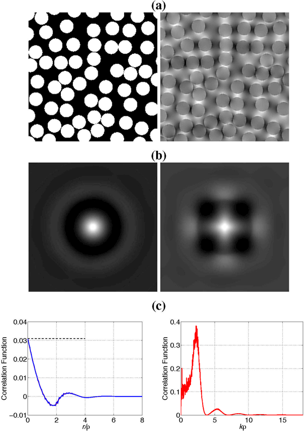
Example of a synthetic two-dimensional medium. (a) The susceptibility profile χ(r) generated by the random self-avoiding addition of disks of radius ρ with a volume fraction ζ = 0.461 and the corresponding Larmor frequency offset $\text{Ω}(\mathbf{r})$ induced by a vertically applied field. (b) Correlation functions ${\text{Γ}}_{\chi }(\mathbf{r})$ and ${\Gamma }_{\text{Ω}}(\mathbf{r})$ of the susceptibility and Larmor frequency, respectively. The images are zoomed 4-fold as compared with (a). (c) Illustration of the locality property in d = 2 dimensions. Left panel: Coinciding angular-averaged correlation functions of the susceptibility ${\text{Γ}}_{\chi }(\mathbf{r})$ (red) rescaled by the factor c₂ = 1/8 (which is the analog of c₃ for two dimensions) and of the Larmor frequency (blue). Dashed horizontal line corresponds to sample variance $\zeta =(1-\zeta )/8$, which is the value of the correlation function at r = 0. Right panel shows the angularaveraged Fourier transform, ${\overline{\text{Γ}}}_{\text{Ω}}(k)$, with the pronounced peak at $k_c\approx 2.3/\rho$. Noise increases for small k due to finite sample effects. Reproduced from (Novikov and Kiselev, 2008).

5.2. Structural correlation functions

The correlation function of a position-dependent quantity ν(r) is defined as⁵

$${\text{Γ}}_{\nu }(\mathbf{r})=\langle \nu ({\mathbf{r}}_0+\mathbf{r})\nu ({\mathbf{r}}_0)\rangle ,$$ (42)

where the averaging is performed over the statistical ensemble of all medium realizations. The quantity ν(r) can be the indicator function of magnetized objects, the magnetic susceptibility, Ω(r) etc. For a sufficiently large sample, the ensemble averaging can be replaced with the averaging over the sample, $\langle \dots \rangle \to \int \text{d}{\mathbf{r}}_0\dots /V$as in Eq. (21). Note that Eqs.(20) and (21) take into account that the mean frequency offset is set to zero, $\langle \text{Ω}(\mathbf{r})\rangle =0$. Performing the Fourier transformation of Eq. (42) with respect to r, by writing $e^{-i\mathbf{q}\mathbf{r}}\equiv e^{-i\mathbf{q}(\mathbf{r}}{}^{{}_0+\mathbf{r})}{e}^i{}^{\mathbf{q}{\mathbf{r}}_0}$ and integrating over $\mathbf{r}\text{'}={\mathbf{r}}_0+\mathbf{r}$ and r₀, yields

$${\text{Γ}}_{\nu }(\mathbf{\text{q}})=\frac{1}{V}\nu (-\mathbf{\text{q}})\nu (\mathbf{\text{q}}).$$ (43)

Examples of correlation functions of χ(r) and ν(r) are given in Fig. 7.

The correlation function has a few convenient properties. First, its q-integral equals the second moment of the correlated quantity (or the variance for the definition sketched in footnote 5),

$${\displaystyle \int \frac{{\text{d}}^{\mathit{\text{d}}}\mathbf{\text{q}}}{{(2\pi )}^{\mathit{\text{d}}}}}{\text{Γ}}_{\nu }(\mathbf{\text{q}})={\text{Γ}}_{\nu }(\mathbf{r}){|}_{\mathbf{r}=0}=\langle {\nu }^2(\mathbf{r})\rangle .$$ (44)

Second, there is a special property of correlation functions for media consisting of individual objects such as shown in Fig. 7. Γ_ν for additive quantities ν such as, for instance, the magnetic field, is mainly determined by the single-object contribution when the volume fraction of the randomly placed objects is low. This can be shown using the Fourier representation, Eq. (43) (cf. Appendix B in (Burcaw et al., 2015)). Applying it to identical objects, $\nu (\mathbf{\text{q}})={\sum }_n{\nu }_1(\mathbf{\text{q}})e^{-i\mathbf{\text{q}}{\mathbf{r}}_n},$

$$\text{Γ}(\mathbf{\text{q}})=\frac{{\nu }_1(\mathbf{\text{q}}){\nu }_1(-\mathbf{\text{q}})}{V}{\displaystyle \sum _{nm}{e}^{i\mathbf{\text{q}}(\mathbf{r}}{}^{{}_n-{\mathbf{r}}_m)}},$$ (45)

where ν₁(q) is the contribution of a single object placed at r = 0 and the indices n and m count all objects. The sum is dominated by the diagonal terms with n = m, while the rest is zero in the limit of totally uncorrelated positions of different objects, which is a good approximation for low volume fractions. The diagonal terms give

$$\text{Γ}(\mathbf{\text{q}})=\frac{N}{V}{\nu }_1(\mathbf{\text{q}}){\nu }_1(-\mathbf{q})=\zeta {\text{Γ}}_{{}_{\nu }}^{(1)}(\mathbf{q}),{\text{Γ}}_{{}_{\nu }}^{(1)}(\mathbf{q})=\frac{{\nu }_1(\mathbf{q}){\nu }_1(-\mathbf{q})}{{\nu }_0},$$ (46)

for N objects, where ν₀ is the volume of a single object and ζ = N_ν0/V is the total volume fraction of objects.

In general, the correlation function gives an overview on the medium structure on all scales. Its value at short distances and, correspondingly, large q, reveals the fine structure of the medium, in particular, the shape |ν₁(q)|² of individual objects shown in Fig. 7. In the opposite limit of long separations and, correspondingly, small q, it is dominated by the double sum in Eq. (45), which is sensitive to the large-scale statistics of the overall medium organization. In particular, the nearly constant value of Γ(q) for q → 0 (a plateau for $k\ll 1/\rho$ in Fig. 7(c), right panel) signifies the absence of long-distance correlations in the medium. Indeed, when an examination of a medium is performed with a low resolution, that is only small values of q are sampled (below 1/ℓ_c), the correlation function Γ(q) appears constant, which corresponds to a delta-functional form of Γ(r) on the scales exceeding the correlation length ℓ_c.

This simple reasoning has implications for the long-time form of the relaxation rate, which turns out to be sensitive to the form of Γ(q) for q → 0 as discussed below in Sec. 5.3. Deviations from the constant value of Γ(q) in this limit are possible, which reflects essential features of the medium structure, an example is discussed in Sec. 5.3.6 below. A general classification of structurally disordered media is given in (Novikov et al., 2014) in the related context of diffusion physics.

5.3. Diffusion-narrowing regime

Here we identify DNR with the perturbative regime (15), where motional narrowing results in

$${\mathit{R}}_2^{\text{meso}}|{}_{t\gg {\tau }_c}\sim \delta {\text{Ω}}^2\cdot {\tau }_c\sim \frac{\delta {\text{Ω}}^2{\text{ℓ}}_c{}^2}{D}.$$ (47)

The condition $\alpha \ll 1$ enables finding the signal perturbatively in α. Technically, there are two major analytical approaches to this problem: the cumulant expansion and the Born series. Below we discuss them in general, then consider the second order of the perturbation theory equivalent to the GPA, and its properties given sufficiently short-range character of the magnetic dipole field, and the sensitivity to the short-scale and long-range details of the medium.

5.3.1. Cumulant expansion versus Born series

The cumulant expansion approach is based on the series (5), where each term, consisting of the corresponding correlation functions $\langle \text{Ω}{(\mathbf{r}(t_1)\dots \text{Ω}(\mathbf{r}(t_n))\rangle }_c,$ can be subsequently averaged over the Brownian paths r(t), in analogy to Eq. (20) above. The lowest nontrivial order (the second order) corresponds to the Gaussian phase distribution $S\sim e^{-\langle {\phi }^2\rangle /2}$, from which the term Gaussian phase approximation originates. The advantage of the cumulant approach is its relative simplicity for obtaining the GPA expressions; the disadvantage is that it does not embed the relaxation physics in a more general context.

The Born series approach involves finding the voxel-averaged Green’s function

$$G(t,\mathbf{q})\equiv {\displaystyle \int \frac{\text{d}{\mathbf{r}}_0\text{d}\mathbf{r}}{V}}\text{𝓖}(t;\mathbf{r},{\mathbf{r}}_0)e^{-i\mathbf{q}(\mathbf{r}-{\mathbf{r}}_0)}$$ (48)

of the mesoscopic Bloch-Torrey equation (34) perturbatively in the term −iΩψ, starting from the pure diffusion propagator, Ω ≡ 0 (analogously to the Born series for the corresponding scattering solution of the Schrӧdinger equation (Landau and Lifshitz, 1981)). The propagator (48) is more complex than the FID signal, as it formally corresponds to the diffusion-weighted signal (with diffusion weighting q created by ideal narrow pulses), cf. the notation and detailed derivations by Novikov and Kiselev (2008, 2010); Kiselev (2017); Novikov et al. (2016). The FID signal is then obtained as S = G(t,q)|_q=0, cf. Eq. (37).

It is obvious at this point that the GPA is equivalent to the second-order perturbation term in the Born series, as both involve terms up to Ω². While applying the Born series for deriving the GPA may seem an overkill, it enables generalizations for α ∼ 1, based on the summation of infinite subsets of contributions to the Born series via the self-consistent treatment of the nonperturbative problem (Novikov and Kiselev, 2008), Sec. 8, as well as establishing the confounding effects of mesoscopic Ω(r) on the apparent diffusion metrics.

5.3.2. The second-order solution

In this Section, we will remain within the GPA, with beyondGPA results briefly reviewed Sec. 8 below. This perturbative treatment enables a lowest-order solution of the central problem of expressing the frequency correlation function J(t), Eq. (8), in terms of the microstructural properties of the considered tissue. The general solution to this problem is obtained by averaging over the random paths with the exact diffusion propagator, 𝓖(t, r, r₀), giving the probability of a particle to move from point r₀ to r in the time interval t:

$$J(t)\equiv {\displaystyle \int \frac{\text{d}{\mathbf{r}}_0\text{d}\mathbf{r}}{V}}\text{Ω}(\mathbf{r}){\text{𝓖}}_0(t,\mathbf{r},{\mathbf{r}}_0)\text{Ω}({\mathbf{r}}_0).$$ (49)

Note that 𝓖₀ in the present context is the solution to the pure diffusion equation (Eq. (34) with ${\mathit{R}}_2^{\text{mol}}(\mathbf{r})$ ≡ 0 and Ω(r) ≡ 0), see the comment after Eq. (37).

Using the approximation of the free diffusion propagator in the q-space, ${\mathcal{𝓖}}_0\to \theta \left(t\right)e^{-\text{D}{\mathbf{q}}^{2}t}$, where θ(t) is a unit step function, yields⁶

$$J(t)=\theta (t){\displaystyle \int \frac{{\text{d}}^3\mathbf{q}}{{(2\pi )}^3}}{\Gamma }_{\text{Ω}}\left(\mathbf{q}\right)e^{-D{q}^{2}t},$$ (50)

where the two-point correlation function is defined according to Eqs. (21) and (43). Equivalently, in the spectral domain

$$J(\omega )={\displaystyle \int \frac{{\text{d}}^3\mathbf{q}}{{(2\pi )}^3}}\frac{{\Gamma }_{\text{Ω}}(\mathbf{q})}{-i\omega +D{q}^2}$$ (51)

(Jensen and Chandra, 2000b; Novikov and Kiselev, 2008).

The instantaneous relaxation rate Eq. (19) is given by the time integration of Eq. (50), obtaining

$${\mathit{R}}_2^{\text{meso}}(t)={\displaystyle \int \frac{{\text{d}}^3\mathbf{q}}{{(2\pi )}^3}}{\Gamma }_{\text{Ω}}(\mathbf{q})\frac{1-e^{-D{q}^{2}t}}{D{q}^2}.$$ (52)

We can immediately see, by Taylor-expanding $1-e^{-\mathit{\text{D}}{q}^{2}t}\simeq \mathit{\text{D}}{q}^{2}t$, that at short t → 0, the rate (52) vanishes as ${\mathit{R}}_2(t)\simeq \langle {\text{Ω}}^2\rangle \cdot t$, in agreement with the universal short-time behavior of the signal (10), where $\langle {\text{Ω}}^2\rangle \equiv {\Gamma }_{\text{Ω}}(\mathbf{r}){|}_{r=0}$ corresponding to inte13 grating Eq. (43) over all q.

The FID signal, following Eq. (19), can be obtained via integrating Eq. (57) one more time:

$$\ln S(t)=-{\mathit{R}}_2^{\text{mol}}t-{\displaystyle \int \frac{{\text{d}}^3\mathbf{q}}{{(2\pi )}^3}}{\Gamma }_{\text{Ω}}(\mathbf{q})\frac{e^{-D{q}^{2}t}-1+D{q}^{2}t}{{(D{q}^2)}^2}.$$ (53)

Here, we added the molecular contribution (the first term). Fea15 tures of the DNR relaxation rate that follow from the above re sults are discussed in the next three subsections.

The generalizations onto SE and CPMG sequences are done according to the recipe given in Sec. 4: The diffusion propagator in Eq. (49) is approximated with a convolution chain of Gaussian propagators with the complex conjugation of the accumulated factors to the moment of each refocusing pulse. This results in the substitution of the numerator under the integral in Eq. (53) with functions g_SE and g_CPMG from Eqs. (11) and (12) of (Kiselev and Novikov, 2002).

5.3.3. Locality in the DNR

Consider now a practically important case of statistically isotropic magnetic media, characterized by the isotropic susceptibility correlation functions

$${\text{Γ}}_{\chi }(r)=\frac{1}{{\chi }_0^2}{\langle \chi ({\mathbf{r}}_0+\mathbf{r})\chi ({\mathbf{r}}_0)\rangle }_{{\mathbf{r}}_0}$$ (54)

that depend only on the absolute value r = |r| (meaning that the magnetic inclusions are packed without any preferred direction). The link to their structure, embodied in the dimensionless function Γ_χ(r), can be made more direct by substituting Ω(q) from Eq. (41) in Eq. (43), and in all successive d³q integrations of this object, yielding $R_2^{\text{meso}}(t)$ and the signal. Since the rest of the integrand in the above equations does not depend on the direction of q, the angular integration the factor ${(1/3-q_z^2/q^2)}^2$ can be performed independently of the rest of the integrand, giving a constant factor

$$c_3={\displaystyle \int \frac{sin\theta \text{d}\theta \text{d}\varphi }{4\pi }}{\left(\frac{1}{3}-{\cos }^2\theta \right)}^2=\frac{4}{45}.$$ (55)

In other words, in a statistically isotropic sample, averaging over the positions and orientations of the susceptibility inclusions becomes decoupled from averaging over the inclusions becomes decoupled from averaging over the Xdirections of the induced dipole field. Practically, this means that we can think in terms of an angular-averaged frequency correlation function

$${\overline{\text{Γ}}}_{\text{Ω}}(\mathit{q})=c_3·\delta {\text{Ω}}^2·{\text{Γ}}_{\chi }(\mathit{q})$$ (56)

that is directly proportional to that of the susceptibility, Γ_χ(q).

The reduction of the susceptibility-induced Larmor frequency correlation function to that of the source of the induced field, the magnetic susceptibility χ(r), was called locality (Novikov and Kiselev, 2008).

The precise statement is that in the second order of the perturbation theory, the diffusion-mediated interaction with the in duced field looks like a completely local interaction with the magnetic structure χ(r) itself (as if it were the term $-i\sqrt{c_3}(\delta \text{Ω}/{\chi }_0)\cdot \chi (\mathbf{r})$ entering the mesoscopic Bloch-Torrey equation (34), instead of −iΩ(r), which is non-local according to Eq. (39)). This enables the sensitivity to the magnetic microstructure In the DNR, rather than to merely the net amount of magnetization.

The physical origin of the locality property is the (almost) local character of the dipole field (40) — namely, it decays as 1/r³, i.e., as the inverse power of the distance that precisely equals the spatial dimensionality — and therefore its Fourier transform Y(q) does not add any powers of q to χ(q), Eq. (41), and subsequently correlation function to its Γ_χ(q), Eq. (43).

5.3.4. Non-universal long-time relaxation rate

The rate (52) in the t → ∞ limit approaches a constant value, cf. Sec. 2.4:

$${\mathit{R}}_2^{\text{meso}}(\infty )=\frac{1}{V}{\displaystyle \int \frac{{\text{d}}^3\mathbf{q}}{{(2\pi )}^3}}\frac{\text{Ω}(\mathbf{q})\text{Ω}(-\mathbf{q})}{D{q}^2},$$ (57)

where we represented the correlation function using Eq. (43). This expression formally maps onto a Coulomb energy

$${\mathit{R}}_2^{\text{meso}}(\infty )=\frac{1}{V}{\displaystyle \int \text{d}\mathbf{r}\text{d}\mathbf{r}\prime }\frac{\text{Ω}(\mathbf{r})\text{Ω}(\mathbf{r}\prime )}{4\pi \mathit{D}|\mathbf{r}-\mathbf{r}\prime |}$$

of interaction between charges distributed as Ω(r), since 1/q² corresponds to the Coulomb interaction potential $1/4\pi |\mathbf{r}-\mathbf{r}\prime |$ in the real space. As discussed by Kiselev and Novikov (2002); in the real space. As discussed by Kiselev and Novikov (2002); Sukstans and Yablonskiykii (2003); Novikov and Kiselev (2008) this mapping can be viewed as a long-range “interaction” be7 tween different susceptibility regions mediated by the spins dif8 fusing over a diverging diffusion length in the t → ∞ limit, where the Coulomb potential is the time-averaged diffusion propagator. This analogy helps us appreciate that the rate (57) is nonuniversal, i.e., it depends on the details of how Ω(r) is distributed in space, rather than, say, merely on its sample variance 〈Ω²〉. The reason for this dependence is the same as the capacitance of a charge distribution depends on the geometry of the conductors. The larger the spatial scale on which Ω(r) is distributed, the larger is the “Coulomb energy” (as it is determined by the large-scale charge inhomogeneities), and the stronger the relaxation rate (the less effective the diffusion narrowing).

5.3.5. Long-time relaxation rate

For the model Gaussian-shaped Γ_Ω(q), Eq. (22), the integration (50) yields the temporal correlation function (23) characterized by the algebraic t^−3/2 decay at long times. This is a direct consequence of the the shortrange nature of Larmor frequency correlations as expressed by the constant limit of the model correlation function function for q → 0. Indeed, for t → ∞, the integral in Eq. (50) converges for small q due to the factor $e^{-D{q}^{2}t}$ thus rendering the specific form of the correlation function for larger q irrelevant. Therefore, the t^−3/2 decay at long times is a common feature for all media with the shortrange disorder (Ruh et al., 2015). An example of a qualitatively different disorder class is given below.

5.3.6. CLT breakdown: A diverging $R_2^{\text{meso}}$(∞)

As discussed in Sec. 5.2, Γ_χ(q) tends to a constant for small q (Fig. 7(c)) in media with with short-range disorder. The behavior of Γ_χ(q), and the corresponding convergence in Eq. (57), are qualitatively different in media built with long elements such as blood vessels or fibrous tissues (“sticks” or cylinders longer than the achievable diffusion length). In such media, a point with a given χ has a corresponding point with the same value on a surface of a large enclosing sphere. The statistical weight of such a perfect correlation is proportional to the solid angle of the correlation spot as seen from the sphere’s origin. This angle scales with an increasing sphere radius r as 1/r², and so does the correlation function decay for large separations. The Fourier transform of 1/r² is proportional to 1/q, which dominates the form of Γ_χ(q) ∼ 1/q, q → 0, for such media, cf. the extended disorder classification by Novikov et al. (2014) for the analogous problem in diffusion. Substitution of such a correlation function in Eq. (57) results in a divergence at q → 0. To analyse this case, we have to step back to Eq. (50) and estimate the integral, which gives the long-time tail J(t) ∼ 1/t in the Larmor frequency correlation function as a result of coarse-graining of the medium. This slow approach to zero results in the logarithmically diverging mesoscopic relaxation rate R₂(t) ∼ ln t, i.e., formally $R_2^{\text{meso}}$ (∞) = ∞, and, correspondingly, ln S(t) ∼ −t ln t (Kiselev and Posse, 1998; Jensen and Chandra, 2000b). Hence, the CLT argument of Sec. 2.4, that guaranteed the finite relaxation rate at t → ∞, breaks down in media with diverging spatial correlations, due to a long-time memory in J(t).

Since this effect is caused by the q → 0 divergence of the correlation function, it may manifest itself in different set tings in particular, it is completely analogous to how the in stantaneous diffusion coefficient approaches its long-time limit, D_inst(t) $\simeq D_{\infty }+A/t$, when diffusion is restricted by long ran- dom obstacles such as in extra-axonal space in brain white mat ter (Burcaw et al., 2015; Novikov et al., 2014; Fieremans et al., 2016). This results in the behavior D(t) ≃ D_∞ + A(ln t)/t for the conventionally used cumulative diffusion coefficient. While of the similar origin, the effect for the diffusion coefficient is less dramatic, as it approaches the constant value D_∞ corresponding to Gaussian diffusion, albeit slowly.

Consider now the spin echo attenuation. According to the meaning of correlation time, dephasing can be refocused for short times, t ≪ τ_c, while the effectiveness of dephasing decreases for t ≳ τ_c. According to the estimate for the FID, ln S ∼ −(δΩτ_c)²t/τ_c in the DNR, the signal attenuation is still minor for t ∼ τ_c due to small α, so that the refocusing in a SE sequence cannot result in a large effect relative to FID. A significant FID attenuation occurs for long times, t ≫ τ_c, for which the phase history is already forgotten; for these t, the re focusing also has a little effect because phase history cannot be recovered, making the spin-echo signal to the moment of the echo time, t_E, only slightly larger than that for the FID. Explicit examples can be found in (Kiselev and Posse, 1998; Kiselev and Novikov, 2002; Sukstanskii and Yablonskiy, 2003, 2004). In particular, the ln t_E divergence occurs in the corresponding SE rate (Kiselev and Posse, 1998).

5.4. Static dephasing regime

Consider now the regime opposite to the DNR, which is the case of α ≫ 1. According to the Central limit theorem, the relaxation becomes monoexponential for long times, t ≫ τ_c, Sec. 2.4. This is, however, of little practical interest, since the signal is strongly attenuated for such long times. The measurable signal attenuation occurs already for the relatively short times, $t~1/\delta \mathrm{\Omega }\ll {\tau }_c$, and hence one might expect that the resulted attenuation does not depend on τ_c. The “short” time can be practically long, for example in a medium with, e.g., large cells, ℓ_c = 20 µm, it is ℓ_c²/D ≈ 400 ms for the typical diffusivity D ≈ 1 µm²/ms. When τ_c becomes very large, the time scale of transverse relaxation $1/R_2^{\text{meso}}$ is parametrically given solely by δΩ⁻¹ ≪ τ_c (no lineshape narrowing).

To make further estimates, it is useful to realize that the smallness of relevant times as compared to τ_c means that the spins experience nearly constant local field, Ω(r), as they do not move appreciably relative to the distance ℓ_c on which it changes. For a transparent definition of “local”, it is convenient to consider the spin packets. A spin packet excited at a point r₀ includes all spins that experienced the initial spin flip at this point, wherever they move afterwards. The whole signal is the sum of magnetizations of all spin packets:

$$S(t)=\frac{1}{V}{\displaystyle \int \text{d}{\mathbf{r}}_0}\text{d}\mathbf{r}𝓖(t;\mathbf{r},{\mathbf{r}}_0)=\frac{1}{V}{\displaystyle \int \text{d}{\mathbf{r}}_0\text{Ψ}({\mathbf{r}}_0}),$$ (58)

where 𝓖(t; r, r₀) is the exact propagator of the Bloch-Torrey equation, Eq. (34), as introduced Sec. 4 and Ψ(r₀) = ∫ dr 𝓖(t; r, r₀) the magnetization of a single spin packet.

In the considered case, the spin packets are narrow as compared with ℓ_c, which justifies the Taylor expansion of the magnetic field near the point r₀:

$$\text{Ω}\left(\mathbf{r}\right)\approx \text{Ω}\left({\mathbf{r}}_0\right)+\nabla \text{Ω}\left({\mathbf{r}}_0\right) \cdot \left(\mathbf{r}-{\mathbf{r}}_0\right)·$$ (59)

Signal evaluation for different pulse sequences goes now essentially different ways. Consider first the FID. Taking into account just the lowest-order term in Eq. (59), the magnetization of a given spin packet takes the form $\text{Ψ}({\chi }_0)=e^{-i\text{Ω}({\mathbf{r}}_0)t}$. Integration over the whole sample gives

$$S(t)=\frac{1}{V}{\displaystyle \int \text{d}{\mathbf{r}}_0}{e}^{-i\text{Ω}({\mathbf{r}}_0)t}\equiv {\displaystyle \int \text{d}\text{Ω}\text{𝒫}(\text{Ω})e^{-i\text{Ω}t}},$$ (60)

cf. Eq. (4), where

$$\text{𝒫}(\text{Ω})\equiv {\displaystyle \int \text{d}{\mathbf{r}}_0\delta }(\text{Ω}-\text{Ω}({\mathbf{r}}_0))$$ (61)

is the properly normalized PDF of the Larmor frequency in the sample (or an MRI voxel). The next-to-leading term in Eq. (59) results in additional attenuation within the spin packets. This slightly increases the relaxation rate; to the best of our knowledge, the only explicit calculation of this FID correction was done for a model of blood vessels (Kiselev and Posse, 1999).

Consider now the signal to be the magnitude of a spin echo, or of a multi-echo sequence such as CPMG. The signal attenuation in the SDR occurs in the regime of short echo times as compared with the correlation time, t ≪ τ_c. This means that this attenuation can be effectively refocused. In more detail, the overall phase of spin packets is zero at the moment of echo, which means that the first term on the right-hand side of Eq. (59) does not contribute to the relaxation and the second term becomes dominant. Physics of relaxation within each spin packet is now the dephasing of spins in a nearly constant gradient ∇Ω(r₀) of Larmor frequency. This is well known in diffusion MRI. The spin packet magnetization can be expressed via the so-called bfactor, Ψ(r₀) = e^−b(r₀)D, with b(r₀) being a local quantity in the current context. Beyond the location, the value of b depends on the applied pulse sequence. For example, for a CPMG sequence with N instant refocusing pulses, the applied pulse sequence. For example, for a CPMG sequence with N instant refocusing pulses,

$$b=\frac{1}{12N^2}{(\nabla \text{Ω})}^2{t}^3,t=N{t}_E·$$ (62)

The b-factor is thus proportional to N, much like in the oscil- lating gradients diffusion measurement. It is clear from this example that the echo attenuation strongly depends on t_E, as opposed to SE or CPMG measurements in a sample without the mesoscopic structure.

Another issue is that there is no guarantee for the monoex ponential relaxation for practically long times, t ≫ δΩ⁻¹, an example is given in Sec. 6.2 below. The dependence of the signal attenuation on time and δΩ for generic heterogeneous media was studied by Jensen and Chandra (2000c).

Neglecting spin motion for the FID justifies the term “static dephasing regime” for the considered case (Yablonskiy and Haacke, 1994). Although the spin echo attenuation is fully due to the motion, the same term is also conventionally applied for the SE case.

6. Low-density suspensions of paramagnetic inclusions

Sparse inclusions that induce a microscopically heteroge neous field is the most studied case in the theory of mesoscopic transverse relaxation. The major advantage is the possibility to perform the averaging over the medium for a rather general case (Yablonskiy and Haacke, 1994). The most prominent application is a quantitative theory of relaxation caused by para magnetic blood in the brain microvasculature (Yablonskiy and Haacke, 1994; Kiselev and Posse, 1998, 1999; Marques and Bowtell, 2008), and of relaxation in the trabecular network in the bone marrow (Yablonskiy and Haacke, 1994; Hwang and Wehrli, 1995; Ma and Wehrli, 1996).

Consider a medium in the volume V that contains N distinct paramagnetic objects randomly placed in space, each of the volume ν₀. The overall volume fraction is ζ = Nv₀/V ≪ 1. Each object induces a Larmor frequency shift, we denote the field induced by the n-th object at a point r as Ω_n(r). This field depends on the position of the object and may include further magnetic field experienced by a given spin is the sum of individual object contributions,

$$\text{Ω}(\mathbf{r})={\displaystyle \sum _n{\text{Ω}}_n}(\mathbf{r})·$$ (63)

Consider first the FID. The magnetization of a given spin packet located at a point r takes the form of a product,

$$\text{Ψ}(\mathbf{r})={\displaystyle \prod _n{\text{Ψ}}_n}(\mathbf{r}-{\mathbf{r}}_n),$$ (64)

where Ψ_n = e^−iΩnt is the effect of a single object. This expression is to be averaged over the positions of all objects. Since all space points become equivalent after the averaging, the signal does not depend on the position r of the considered spin packet. The averaging gives the signal in the form

$$S(t)={\displaystyle \int \text{d}{\mathbf{r}}_1}\dots \text{d}{\mathbf{r}}_{N}P({\mathbf{r}}_1\dots {\mathbf{r}}_N){\displaystyle \prod _n{\text{Ψ}}_n}(\mathbf{r}-{\mathbf{r}}_n),$$ (65)

where P(r₁…r_N) is the probability of a given configuration of all objects. This expression is exact, but extremely difficult to work with. The low volume fraction ζ ≪ 1 justifies a simplification to treat the objects as statistically independent, in particular, each of them having a uniform probability to be at any position inside the volume, V. In this way, we incorrectly account for configurations with overlapping objects, but the statistical weight of such configurations is negligible, ∼ ζ², while we are going to evaluate effects of the order of ζ. With this accuracy, P(r₁…r_N) = 1/V^N and the signal can be fully factorized in the product of individual objects (Yablonskiy and Haacke, 1994):

$$S(t)={\displaystyle \prod _n\left[{\displaystyle \int \frac{\text{d}{\mathbf{r}}_n}{V}{\text{Ψ}}_n(\mathbf{r}-{\mathbf{r}}_n)}\right]}={\left[{\displaystyle \int \frac{\text{d}{\mathbf{r}}_1}{V}{\text{Ψ}}_1(\mathbf{r}-{\mathbf{r}}_1)}\right]}^N\equiv S_1^N·$$ (66)

The second equality is written for identical objects, a straight2 forward generalization for non-identical ones is described be3 low. Finding the signal is thus reduced to the considering the effect of a single paramagnetic object.

The spin packed magnetization Ψ₁(t,r) under the influence of a single object is a function of the object’s position, r₁. This function is unity everywhere except for an area close to the spin packet. To single out the non-trivial effect, we use an identity Ψ₁ = 1 − (1 − Ψ₁), which results in

$$S_1(t)=1-\frac{{\nu }_0}{V}{\displaystyle \int \frac{\text{d}{\mathbf{r}}_1}{{\nu }_0}}\left[1-{\text{Ψ}}_1({\mathbf{r}}_1)\right]\equiv 1-\frac{{\nu }_0}{V}f(t),$$ (67)

where we introduce a dephasing function,

$$f(t)={\displaystyle \int \frac{\text{d}{\mathbf{r}}_1}{{\nu }_0}}\left[1-{\text{Ψ}}_1({\mathbf{r}}_1)\right]$$ (68)

and used the symmetry of Ψ(r − r₁) with respect to interchanging r and r₁. The total signal in the limit N → ∞ is then (Yablonskiy and Haacke, 1994)

$$S(t)={\left[1-\frac{{\nu }_0}{V}f(t)\right]}^N\simeq e^{-\zeta f\left(t\right)}·$$ (69)

Considering non-identical objects (for example, those with different size or orientations in space), we can subject the groups of identical objects to the above consideration, which gives a product of factors e^−ζf(t) for each group. This is equivalent to the summation (integration) in the exponential. We thus conclude that the dephasing function includes the integration over all inherent properties of paramagnetic object (other than their location in space).

Two more remarks are in order. First, note that the integration in Eq. (68) spans the whole space. This is incorrect for objects that are impermeable for spins; their own volume should be excluded from integration, which can be formally done by setting Ψ = 1 (no relaxation) inside the objects. Second, the applied method is known in statistical physics as the virial expansion, which is a way to find corrections to the properties of a nearly ideal gas due to the interaction between its molecules (see, e.g., (Feynman, 1998)). The first correction takes into account the pairwise interaction between the molecules neglecting the multi-particle interactions, which is mapped in our case ing the multi-particle interactions, which is mapped in our case paramagnetic object separately, neglecting interactions between them (such as, in particular, the non-overlapping condition).

While Eq. (69) is justified by the only condition ζ ≪ 1, the spin packet magnetization, Ψ₁, can be evaluated using further approximations. In what follows, we consider the application of diffusion narrowing and static dephasing regimes for this purpose.

6.1. Diffusion narrowing regime

In the DNR, the perturbation theory can be used to calculate the dephasing function, Eq. (68). The result can be expressed in the form similar to Eq. (53), but with the correlation function of the field induced by a single object, Eq. (46) (Kiselev and Novikov, 2002).

In this way, the relaxation effect of suspensions of magnetized objects with regular shapes has been calculated.In particular, Gillis and Koenig (1987) calculated the mesoscopic contribution to R₂(∞) for impermeable spheres; Kiselev and Posse (1998) calculated signal attenuation for permeable cylinders for all t; and Jensen and Chandra (2000b) calculated the mesoscopic contribution to R₂(t) for permeable spheres for all t. Kiselev and Novikov (2002) demonstrated the sensitivity of the FID, spin echo and CPMG signals to the objects’ shape, via calculating the corresponding signals for permeable cylin ders of arbitrary aspect ratio and for permeable spheres for all echo times. The fact that objects’ shape matters can be intu itively understood by invoking the discussed earlier similarity of the low-frequency expression, Eq. (57), with the electrostatic energy (Kiselev and Novikov, 2002; Sukstanskii and Yablon skiy, 2003; Novikov and Kiselev, 2008). Finally, Sukstanskii and Yablonskiy (2003) re-expressed the solution of (Kiselev and Posse, 1998) in terms of a hypergeometric function, and found explicit expressions for the FID and spin echo signals in the permeable-sphere model of Jensen and Chandra (2000b). Sukstanskii and Yablonskiy (2004) found the FID and spin echo signals for the dilute suspension of impermeable spheres and cylinders in the GPA. Note that the results for permeable and impermeable cylinders are numerically very close to each other, as are the results for the spheres (Fig. 5).

The DNR relaxation rate can be obtained directly from Eq. (50) or any equivalent formulation. To see that, use the reduction of the correlation function to that of single objects, Eq. (46).

6.2. Static dephasing regime

For the following, we need the parametric form of the scaling with the distance r

$$\text{Ω}(\mathbf{r})\sim \frac{{\rho }^d}{r^d}\cdot \delta \text{Ω}$$ (70)

of magnetic field induced by spheres of radius ρ in d dimensions (d = 2 refers to a cylinder in the orthogonal cross-section; d = 1 is a slab of thickness 2ρ, inifinite in both directions); here δΩ is the typical field on the sphere’s surface. The spin dephasing develops as the time goes on. Since the field is stronger closer to the sphere, the volume adjacent to the sphere will be dephased first. The relaxation can thus be qualitatively considered as the increase in the dephased volume.

Let us estimate how this dephased volume grows with time t. For the estimate, we replace the smooth transition from Ψ ≪ 1 close to the sphere surface to Ψ = 1 far from it with a sharp boundary between the fully dephased and non-dephased volumes. The size of the dephased volume is determined by the requirement $\text{Ω}(\mathit{r})\cdot t\gtrsim 1$, which gives r^d ∼ ρ^dδΩt for its radius r(t). Using Eq. (68) with ν₀ ∼ ρ^d, we obtain for the long-time asymptotic regime

$$f=\frac{r^d}{{\rho }^d}=c_{\text{FID}}\delta \text{Ω}t,$$ (71)

where c_FID is a numerical constant. This simple result proves that the FID signal in the SDR decays exponentially with t at long t with the rate ${\mathit{R}}_2^{\text{meso}}(\infty )\sim \zeta \delta \Omega$, and also reveals the meaning of the dephasing function as the ratio of the dephased volume to the object’s volume. Accurate calculations are available for spheres, randomly placed parallel cylinders and randomly placed and oriented cylinders (Yablonskiy and Haacke, 1994).

It is instructive to justify the applicability of the SDR to the problem at hand. It would be straightforward to estimate the field correlation length as the object size, ρ and require it to be shorter than the diffusion length, (Dt)^1/2. This condition would however break for some time of the order of ${\tau }_c\sim {\rho }^2/D$. This estimate is too strict because the precise form of the low magnetization inside the dephased volume is not essential. It is important that the diffusion length is comparably short at the boundary of the dephased volume whose increase with time determines the relaxation rate. This results in the requirement $Dt\ll r^2\sim {\rho }^2{(\delta \text{Ω}t)}^{2/\text{d}}$. In two dimensions, time cancels, and the SDR applicability condition becomes $\delta \text{Ω}{\tau }_c\gg 1$. In three dimensions, the diffusion length increases faster than the size of dephased volume and overtakes it at $t\sim {\tau }_c{(\delta \text{Ω}{\tau }_c)}^2$. Since the dephasing function is large for such times, $f\sim {(\delta \text{Ω}{\tau }_c)}^3$, this regime can be observed for extremely low volume fractions, such that the signal $e^{-\zeta f}$ is not too small.

Consider now the spin echoes. Dephasing occurs within each spin packet rather than between them. The above estimate is modified so that the radius of the dephased volume is estimated as $\mathit{bD}\sim 1$, where $b\sim {(\nabla \text{Ω})}^2{t}^3$ for the Hahn spin echo. With account for Eq. (70), ${\mathit{r}}^{2d+2}\sim {(\delta \text{Ω}t)}^2{\rho }^{2d}Dt$. This gives

$$f(t)=c_{\text{SE}}^{(2d)}\frac{\delta \text{Ω}t}{{(\delta \text{Ω}{\tau }_c)}^{1/3}},\delta \text{Ω}{\tau }_c\gg 1,d=2,$$ (72)

$$f(t)=c_{\text{SE}}^{(3d)}\frac{{(\delta \text{Ω}t)}^{9/8}}{{(\delta \text{Ω}{\tau }_c)}^{3/8}},\frac{{(\delta \text{Ω}{\tau }_c)}^3}{\delta \text{Ω}t}\gg 1,d=3·$$ (73)

Similar to the FID, the SDR for the SE in three dimensions breaks down for very long times, t ∼ τ_c(δΩτ_c)², for which f ≫ 1. Note that the non-monoexponential relaxation in three dimensions, f ∼ t^9/8, agrees with the general estimation based on the scaling analysis (Jensen and Chandra, 2000c).

The above picture of dephased volumes around paramagnetic objects implies not much dependence of relaxation on details of the object’s shape for long times. This is based on the multipole expansion according to which the field from any object at large distances from the object is approximated by the dipole field; corrections due to deviation from this form are cur rently unknown.

7. Effective medium theory

In physics, effective medium theory (EMT) is an approach to describing properties of heterogeneous media in terms similar to those used for homogeneous media. In this way, the quantities describing medium properties become dispersive (frequency dependent). As an example, consider light propagation in a medium. While the interaction of light with medium’s molecules may be very complicated to describe, light propagation on the macroscopic scale is fully determined by the complex-valued dispersive refraction index. The problem of light propagation thus decouples into two problems: (i) To find the refraction index given the atomic medium composition and (ii) to find the light propagation given a refraction index. While the former poses a fundamental challenge, the latter is practically relevant for development of optical devices. The refraction index can be measured as a characteristic of a given medium without reference to its structure on the molecular level.

In the current context, EMT is a framework for representing the transverse relaxation and diffusion for arbitrary disordered magnetic media (Novikov and Kiselev, 2008, 2010). Consider the conventional (molecular) monoexponential FID in the form

$$S(t)=\theta (t)e^{-{\mathit{R}}_2^{\text{mo}{\text{l}}_t}}\iff S(\omega )=\frac{1}{-i\omega +{\mathit{R}}_2^{\text{mol}}}·$$ (74)

The contribution of mesoscopic scale can be summarized as additional dispersive relaxation rate, which is the most straightforward to find in the spectral domain,

$$S(\omega )=\frac{1}{-i\omega +{\mathit{R}}_2^{\text{mol}}+{ℛ}_2(\omega )},$$ (75)

where ℛ₂(ω) collects all effects of mesoscopic dephasing; it peaks at the characteristic frequency 1/τ_c (Novikov and Kiselev, 2008). The inverse Fourier transformation of ℛ₂(ω) equals $\text{d}{R}_2^{\text{meso}}/\text{d}t$, the time derivative of the instantaneous relaxation rate (19); equivalently, at the order α² , ℛ₂(ω) coincides with J(ω), Eq. (51), as it can be seen directly by Taylor-expanding the geometric series (75) in the powers of ℛ₂(ω)/(−iω) (neglecting $R_2^{\text{mol}}$ for the purely mesoscopic contribution).

An advantage of the EMT signal representation (75) is the existence of a well-defined perturbative expansion in the powers of α, Eq. (14), with the first term similar to Eq. (51). It is clear that such a central quantity cannot be found in general. Practically useful is the perturbative approach in which the series in α is approximated by a few first terms, or self-consistently.

8. Self-consistent approximations

The flip side of well-controlled approximations such as the perturbative approach is a limited parametric range such as α ≪ 1. Extending the validity range beyond such limits can be done with the so-called self-consistent approximations. Developing such approximations implies catching essential features of the signal by using intuition rather than strict mathematical apparatus. We sketch here two examples of such approaches.

8.1. Strong collision approximation

In the strong collision approximation (Dattagupta and Blume, 1974), modified for calculating the relaxation effect of parallel paramagnetic blood vessels (Bauer et al., 1999b,a), the tissue is parcellated to the cylindrical volumes affected by individual capillaries, the Krogh’s cylinders (cf. Sec. 10.3 below). The frequency correlation function (8) is assumed to be exponential, e^−t/τc with the time constant, τ_c estimated by considering diffusion motion in the cross-section of the paramagnetic cylinder with no further simplification. On the other hand, the diffusion propagator is replaced by the function describing the exponential decrease in the probability to stay at the initial point with an equal probability to move anywhere within the Krogh’s cylinder,

$$\text{𝓖}(t;\mathbf{r},{\mathbf{r}}_0)=e^{-\lambda t}\delta (\mathbf{r}-{\mathbf{r}}_0)+\frac{1-e^{-\lambda t}}{V},$$ (76)

where V is proportional to the cross-sectional area of the cylin11 der. The self-consistency is imposed by the requirement that this propagator reproduces the correlation time, τ_c, of the field fluctuations experienced by moving spins, which results in λ = 1/τ_c with the signal form found from Eq. (76). In other words, this approximation substitutes diffusion-limited sampling of magnetic microstructure by the exchange between different Larmor frequencies occurring everywhere in the sample with the same rate 1/τ_c; this can be realized as an extension of the Kärger model to an infinite number of exchanging sites.

The strong collision approximation involves a number of uncontrolled assumptions, in particular, the form of the correlation function J(t) in reality is not exponential, but a power-law, Eq. (23), due to a finite density of diffusive eigenstates (unless the objects, such as the blood vessels, are arranged in a regular lattice). On the other hand, this approach demonstrates a good accuracy in comparison with theMonte Carlo simulations (Dickson et al., 2011), with the main advantage of covering the transition between the SDR and the DNR. Perhaps, this ability is due to the form of the propagator, Eq. (76), that combines the SDR feature of staying at the initial point with the DNR feature of moving far from it during the signal decay. A detailed investigation of the approximation accuracy is yet to be done.

8.2. Self-consistent Born approximation

The formalism of effective medium theory can be used to extend the validity range to $\alpha \underset{\sim }{<}1$ using the so-called self-consistent Born approximation, developed within condensed matter physics (Novikov and Kiselev, 2008). To give an idea, in view of the tight connection between the signal and the propagator of the Bloch-Torrey equation discussed in Sec. 5.3.1, the signal form, Eq.(75), implies a similar form of the propagator with the mesoscopic contribution in the denominator (Novikov and Kiselev, 2010). With a simplifying (not strictly justified) ansatz for the mesoscopic contribution, the self-consistency requirement takes the form

$${\mathcal{R}}_2(\omega )={\displaystyle \int \frac{d^3\mathbf{k}}{{(2\pi )}^3}}\frac{{\Gamma }_{\text{Ω}}(\mathbf{k})}{-i\omega +D{k}^2+{\mathcal{R}}_2(\omega )}·$$ (77)

Calculating the integral with a specific form of the frequency correlation function results in an equation from which ℛ₂(ω) can be found. In particular, the presence of a pronounced length scale in bulk blood was taken into account as a sharp peak in angular-averaged $\overline{\text{Γ}}\text{Ω}\left(k\right)$ for a given radius k (Novikov and Kiselev, 2008), which resulted in an extension of the perturbative results towards $\alpha \underset{\sim }{<}1$; the resulting ℛ₂(ω) interpolates between the DNR scaling ℛ₂(ω) ∼ α² for α ≪ 1, and the SDR scaling ℛ₂(ω) ∼ α for larger α. This solution described the line shape of bulk blood reasonably well with two adjustable parameters, ℓ_c and δΩ, corresponding to the erythrocyte size and its magnetic susceptibility.

9. Applications

9.1. Blood in vitro

Transverse relaxation rate in deoxygenated blood quadratically depends on the magnetic field in the range 0.05–1.5T(Brooks et al., 1995), which agrees with the above estimate, Eq. (47). A noticeable quadratic component was also observed in the dependence on the blood oxygen saturation (Spees and Yablonskiy, 2001) and the concentration of a paramagnetic contrast agent (van Osch et al., 2003) in the field 1.5T .

The relaxation rate in whole blood essentially depends on the echo time (the interecho interval) of a CPMG pulse se- quence (Gomori et al., 1987; Ye and Allen, 1995; Gillis et al., 1995). This agrees with the non-negligible correlation time, τ_c, for water diffusion in the dense medium formed by red blood cells. A lower bound on this time can be estimated using the shortest erythrocyte dimension of 2 µm and the plasma diffusivity of 2.20µm²/ms (Li et al., 1998), which gives 2 ms; us ing larger dimensions and averaged diffusivity increases this estimate to a few tens of milliseconds, which explains the pronounced dependence on the echo time.

The above-discussed dependence on the shape of paramagnetic objects was observed experimentally by manipulating the osmotic pressure in blood (Ye and Allen, 1995; Gillis et al., 1995). The effect is strong; the relaxation rate changes about five-fold when the erythrocyte shape varies from compressed discs to spheres keeping the same overall excess of the cell magnetic moment (Gillis et al., 1995).

The spectral shape of water in blood doped with a paramagnetic contrast agent significantly deviates from Lorentzian (Bjørnerud et al., 2000). This line shape can be reproduced the oretically using the self-consistent Born approximation, Sec. 8.2, with two adjustable parameters, which yields realistic red blood cell size and magnetization (Novikov and Kiselev, 2008).

Summarizing, theoretical prediction based on perturbation theory are in a good agreement with experimental data for α ≪ 1 (Jensen and Chandra, 2000b; Kiselev and Novikov, 2002); this was also shown by Jensen et al. (2006) for a Sephadex spheres’ phantom. A good quantitative agreement, even for larger α, can be reached using α and τ_c as fitting parameters (Jensen and Chandra, 2000b; Kiselev and Novikov, 2002; Novikov and Kiselev, 2008). However, fitting has a limited predictive power for the involved parameters, which often can be defined only as order-of-magnitude estimates. In particular, the sensitivity to the cell shape introduces an additional hard-to-control degree of freedom, which can be re-attributed to other parameters when fitting models with fixed object shapes.

9.2. Perfusion measurement

A good understanding of relaxation mechanisms is crucial for measurements of brain perfusion using dynamic susceptibil ity contrast (DSC) MRI (Østergaard et al., 1996b,a). While the While the tracer kinetic theory, which is central for this technique, is formulated in terms of the tracer concentration in blood, the MRI measured quantity is the signal attenuation due to the param21 agnetic tracer, Fig. 8. In the brain with the intact blood-brain barrier (BBB), the tracer stays in the blood vessels that become sources of induced magnetic field thus causing dephasing of proton spins in the surrounding tissue. The magnitude of this effect can be estimated using the data shown in Fig. 8. In the bolus peak, both signals drop down to 57% of their respective pre-bolus baselines. This corresponds to the increase in the relaxation rate by 27 s⁻¹ $(t_E^{\text{GE}}=21\text{ ms})$ and 7s⁻¹ $(t_E^{\text{SE}}=80\text{ ms})$ for the gradient echo and spin echo, respectively. In view of the compartmentalization of contrast to blood vessels, the maximal effect of the relaxation on the molecular level, ${\mathit{R}}_2^{\text{mol}}$, would be a complete suppression of signal from blood in which the contrast agent is compartmentalized. This follows from the short (molecular) range of interaction of paramagnetic ions with water molecules and from the fast water exchange between the plasma and erythrocytes. Taking into account the almost homogeneous proton density in the brain, this leads to the conclusion that the molecular relaxation effect of contrast agent results in a relative signal change of the order of the cerebral blood volume fraction, ζ , which is about 6%. The residual 51% signal change is due to the mesoscopic effect of contrast agent; the contrast agent effect spreads far outside the intravascular compartment via the induced magnetic field. We thus come to the conclusion that the mesoscopic contribution is responsible for a major part (almost 90%) of the signal variation observed in DSC MRI.

Figure 8:

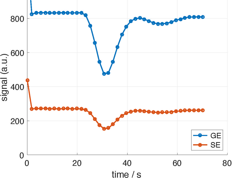
Gradient echo (FID) and spin echo signals averaged over the brain parenchyma in a patient receiving clinical perfusion measurement with a contrast bolus injection. The bolus passage through the brain results in a significant transient signal reduction.

The complex dependence of mesoscopic relaxation on the tissue structure might be a curse or a blessing. On the one hand, it essentially complicates interpretation of investigations with exogenous contrast agent, in particular, evaluation of cerebral perfusion using the dynamic susceptibility contrast (data shown in Fig. 8 were obtained in such an investigation; the noise level is strongly reduced by the performed volume averaging). The main problem is the irrelevance of the relaxivity of contrast agent obtained in-vitro in blood for such a measurement due to completely different spatial distribution of contrast agent when confined in the microvascular system (Kiselev, 2001, 2005). The relaxation rate dependence on the contrast concentration in bulk blood is non-linear (van Osch et al., 2003), which further complicates data interpretation. As mentioned above, the spin-echo relaxation depends in a complicated way on several relevant parameters.

On the other hand, understanding the mechanism of transverse relaxation opens a way to access cellular properties in vivo, a kind of “superresolution”, two – three orders of magnitude below the nominal image resolution. This is completely analogous to considerable current efforts of quantifying tissue microstructure with diffusion MRI using biophysical modeling (Jones, 2010; Novikov et al., 2016). As an example, we discuss below the vessel size imaging, a method for evaluating the mean capillary caliber of the order of 10 μm using imaging with about 2 mm resolution. Further applications encompasses evaluation of the oxygen extraction fraction in the brain microvasculature using a detailed approach to the transverse relaxation induced by oxygenated blood (Sec 9.4 below)

We briefly mention dynamic contrast enhanced (DCE) MRI, which a technique based on T₁ contrast for evaluating the integrity of the BBB and the blood – tissue exchange in other organs. The local longitudinal relaxation effect of contrast agent helps quantifying such measurements. However, it is currently unknown what is the microstructural information available via the transverse relaxation in the presence of a contrast agent in the interstitium.

9.3. Vessel size imaging

The shape dependence of transverse relaxation, in particular, the dependence on the correlation time results in distinct dependences of the FID (measurable with gradient-echo techniques) and the spin-echo transverse relaxation rates on the size of paramagnetic blood vessels, Fig. 9. Simultaneous measurement of both signals enables evaluation of specifically averaged caliber of microvessels (Dennie et al., 1998; Jensen and Chandra, 2000a; Troprès et al., 2001; Kiselev et al., 2005) called vessel size imaging (VSI), see also recent reviews (Troprès et al., 2015; Kiselev and Schmiedeskamp, 2016) and references there in.

Figure 9:

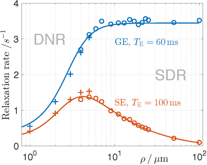
Mesoscopic gradient echo and spin echo relaxation rates as functions of vessel radius in a synthetic medium consisting of straight long monosized cylinders with account for intravascular blood. Symbols show the result of Monte Carlo simulations (Boxerman et al., 1995) for permeable (crosses) and impermeable (circles) vessels. The lines show an interpolation between the known limiting cases (Yablonskiy and Haacke, 1994; Kiselev and Posse, 1998, 1999). The blood volume fraction is kept fixed, ζ = 0.02 for all $\rho$, the blood magnetic susceptibility, $\chi ={10}^{-7}$(cgs), B₀ = 1.5T and the water diffusivity D = 1 μm²/ms.

To summarize the VSI outcomes, the evaluated vessel size appreciably increases in tumors and responds to anti-angiogenic treatment (the majority of observations are pre-clinical). Note that while the vessel size typically correlates with the blood volume in the major part of the brain, these two biomarkers decouple when responding to such treatment. The vessel size often, ple when responding to such treatment. The vessel size often, but not always increases, which is consistent with the preva lent loss of small vessels. In the post-acute ischemic stroke, the vessel size changes, possibly reflecting the microvascular plasticity. For applications in healthy subjects, the method was extended for the use of native paramagnetism of blood under physiological challenges such as inhaling carbon dioxide.

Motivated by different contrast distribution between arteries and veins in the incoming and outgoing bolus (Kiselev et al.,2005), Xu et al. (2012) obtained information about the arterio18 venous composition of microvasculature by comparing the two parts of the bolus. Emblem et al. (2013) reproduced the findings of (Xu et al., 2012) and found a correlation between the therapy response of this composition with the prolonged survival of glioblastoma patients (in this publication, the method was re-coined as “vessel architecture imaging”).

9.4. Mapping oxygen extraction fraction

Understanding transverse relaxation mechanism enables non-invasive evaluation of averaged oxygen extraction fraction using the native paramagnetism of deoxyhemoglobin, the so-called qBOLD method (He and Yablonskiy, 2007; Dickson et al., 2011), see also a recent review (Yablonskiy et al., 2013). Oxygen sat uration obtained in this way correlates well with the direct gas analysis of blood drown from the sagittal sinus of experimental animals (He et al., 2008; Christen et al., 2011). The method was adapted to clinical requirements in a study conducted in human subjects (Domsch et al., 2014).

10. Common misconceptions

10.1. ${\mathit{R}}_2^{\prime }$

It is common to describe the relation between the transverse relaxation rates of the gradient echo (FID) using Eq. (27). This formula originates from NMR in chemical solutions that lack the mesoscopic contribution. While this formula applies for such uniform media, it breaks down in the presence of micrometer- level magnetic structure, in particular, for biological tissues. In such media, Eq. (28) should be replaced with Eqs. (29) and (30) to account for the contribution of all three involved spatiotemporal scales shown in Fig. 1.

The relaxation rate contributions ${\mathit{R}}_{2GE}^{\text{meso}}(t)$ and ${\mathit{R}}_{2SE}^{\text{meso}}(t)$ depend on the magnetic microstructure in a distinct way, as in the relevant example for the vasculature in Fig. 9. As discussed above, these relaxation rates also depend on the details of the applied pulse sequence, in particular the echo time. The presence of these terms, with a complex dependence on all involved parameters, invalidates the simplistic decomposition of Eq. (28), in which ${\mathit{R}}_2^{\prime }$ is assigned the role of accounting for all reversible processes, without the realization that the “reversibility” depends on the ratio of the diffusion length to the object size, and therefore, on the echo time. The adequate picture should be that of Fig. 9 in which the so-called ${\mathit{R}}_2^{*}$ has the complex composition shown in Fig. 3, with ln S (t) having a constantly increasing slope as function of the echo time, and the truly irreversible (molecular) ${\mathit{R}}_2^{\text{mol}}$ given by the initial slope, cf. Eq. (31). The so-called R₂, that is the spin-echo relaxation shows even more complex behavior due to the presence of additional parameters, the timing of the refocusing pulses, cf. discussion below.

Using the inadequate relation (28) yields the estimated ${\mathit{R}}_2^{\prime }$ values that depend on the homogeneity of the main magnetic field, but simultaneously on the tissue morphology and on the details of the applied pulse sequence. Note that these mesoscopic contributions do not need to be small, and can often be dominant, e.g., as discussed in Sec. 9.2.

Hence, the commonly used definitions “${\mathit{R}}_2^{*}$-weighted or R₂-weighted image” can only be accepted as a description of the measurement sequence, according to its unambiguous contrast in homogeneous samples, for which Eq. (28) is valid. This description is, however, incomplete in the context of in vivo MRI.

10.2. SE versus CPMG

Kennan et al. (1994) warned about the need to augment Eq. (28) as early as in 1994. However, the ethos of this equation seems to be still present today. This may be one of the contributing factors to a poor reproducibility of in vivo SE measurements across different sites: At finite echo time, some mesoscopic contributions are unavoidable, and comparing the results across sites and vendors must occur for the same echo time.

Moreover, it is a common rookie error, when, e.g., performing vessel size imaging, to replace the spin echo with the fast spin echo, turbo spin echo or RARE (depending on the scanner manufacturer). While convenient for shortening the measurement protocol, these CPMG-based pulse sequences result in a different relaxation in biological tissues as compared with the Hahn spin echo for which the underlying theory is developed (Eq. (72) and Fig. 9). Since the difference is absent in homogeneous fluids for which Eq. (28) with its inherent interpretation is valid, testing the sequences in commonly used water phantoms cannot reveal the problem.

A good practice would be to introduce reproducible magnetic microstructure phantoms, such as those made of packed synthetic beads (Jensen et al., 2006; Ruh et al., 2015, 2017; Storey et al., 2015), — a practice that is becoming much more common in the area of quantitative diffusion MRI, cf. the review article of Fieremans and Lee in the same journal issue.

10.3. Reduction to single objects

The reduction of the relaxation rate in dilute suspensions to the effect of a single paramagnetic object is often interpreted in the geometric sense that each spin experiences solely the field of the nearest object. In particular, the construction of the Krogh cylinders is recalled when dealing with the relaxation caused by microvasculature. The Krogh cylinder is the result of parcellation the whole tissue in volumes supplied by a single capillary. It is modeled as a cylindrical volume coaxial with a straight cylindrical capillary. This model is justified for the supply with metabolites because this process is mediated by diffusion, which results in an exponential decrease in the metabolite concentration far from the source. In contrast, the magnetic field induced by a paramagnetic object is long-ranged, decreasing as the separation ${\mathit{r}}^{-d}$, where d is the effective number of spatial dimensions (e.g., d = 2 for the long cylindrical blood vessels). Since the number of remote objects increases in proportion to ${\mathit{r}}^d$, the integration over the whole medium cannot be simply limited to the vicinity of a single object. This is reflected in considering the sum over all objects in Eq. (63) and working with the product in the subsequent expressions. Using one cell of the parcellated medium (e.g., the Krogh cylinder) as the representative for the transverse relaxation in the whole medium is justified only for weak signal dephasing, ζ f(t) ≪ 1.

For generalmagneticmicrostructure arrangements, one should directly model the overall correlation functions of the Larmor frequency, which generally do not reduce to a sum of those for the individual objects.

11. Unresolved problems

As illustrated in Fig. 6, transverse relaxation in a few practically relevant cases falls in the intermediate regime between the diffusion narrowing and the static dephasing. Development of adequate theory for this intermediate regime remains a major challenge today. The self-consistent approximations (Sec. 8) may help address this problem, but their development has not yet been given enough time and attention, and their validity range is not well understood yet.

One can also question the reduction of the whole parameter plane in Fig. 6 to only two domains. A hint on a non-trivial relaxation behavior is given by Eq. (73). The signal behavior $\text{ln}S(t)\sim -t^{9/8}$ for long times up to $t\sim {\tau }_c{(\delta \text{Ω}{\tau }_c)}^2\gg {\tau }_c$ appears contradicting the conclusion about the monoexponential decay for $t\gg {\tau }_c$ as a consequence of the CLT. In the considered case, the monoexponential decay takes place in the strongly dephased region close to the paramagnetic object, which does not contribute to f (t). The relevant contribution comes from the size of the dephased region, which renders the relevant correlation time larger than the straightforwardly defined ${\tau }_c$.

Further nontrivial reasons for the CLT breakdown (and, as a result, non-monoexponential relaxation) could originate from collective dephasing effects by rare optimal arrangement of many magnetized objects, and/or the anomalously long-range correlation functions ${\text{Γ}}_{\chi }$ (r). Likewise, parsimonious parametrizations of such correlation functions, that could incorporate both the individual object size/shape and their long-range spatial correlations in real biological tissues (such as for the ferritin), are also still generally missing.

Finally, comprehensively including non-Gaussian diffusion in the cellular environment, and the diffusion anisotropy, e.g., in the white matter, has still yet to be performed.

The above problems map on the current challenge to quantify at least the strongest sources of the mesoscopic dephasing, such as iron depositions or the contrast agent leakage in the interstitium, in terms of the cellular structure. The list of applications of the mesoscopic transverse relaxation modeling can be continued, and we hope that this review article will contribute to their solution and clinical translation.

References

- Abragam A, 1961. Principles of Nuclear Magnetism Oxford University Press, New York. [Google Scholar]
- Anderson PW, Weiss PR, January 1953. Exchange Narrowing in Paramagnetic Resonance. Reviews of Modern Physics 25 (1), 269–276. URL https://link.aps.org/doi/10.1103/RevModPhys.25.269 [Google Scholar]
- Basser P, Mattiello J, LeBihan D, 1994. Estimation Of The Effective Self-Diffusion Tensor From The NMR Spin-Echo. Journal of Magnetic Resonance Series B 103, 247–254. [DOI] [PubMed] [Google Scholar]
- Bauer W, Nadler W, Bock M, Schad L, Wacker C, Hartlep A, Ertl G,12 December 1999a. The relationship between the BOLD-induced T(2) and T(2)(*): a theoretical approach for the vasculature of myocardium. Magn ResonMed 42 (6), 1004–10. [DOI] [PubMed] [Google Scholar]
- Bauer WR, Nadler W, Bock M, Schad LR,Wacker C, Hartlep A, Ertl G, 1999b. Theory of coherent and incoherent nuclear spin dephasing in the heart. Phys. Rev. Lett 83, 4215 – 4218. [Google Scholar]
- Belliveau JW, Kennedy DN, McKinstry RC, Buchbinder BR, Weis skoff RM, Cohen MS, Vevea JM, Brady TJ, Rosen BR, November 1991. Functional mapping of the human visual cortex by magnetic resonance imaging. Science (New York, N.Y.) 254 (5032), 716–9. URL http://www.ncbi.nlm.nih.gov/pubmed/1948051 [DOI] [PubMed] [Google Scholar]
- Bjørnerud A, Briley-Saebø K, Johansson LO, Kellar KE, November 2000. Effect of NC100150 injection on the (1)H NMR linewidth of human whole blood ex vivo: dependency on blood oxygen tension. Magn Reson Med 44 (5), 803–807. [DOI] [PubMed] [Google Scholar]
- Bloembergen N, Purcell EM, Pound RV, 1948. Relaxation Effects in NuclearMagnetic Resonance Absorption. Physical Review 73 (7), 679–712. [Google Scholar]
- Boxerman JL, Hamberg LM, Rosen BR, Weisskoff RM, October 1995. MR contrast due to intravascular magnetic susceptibility perturbations. Magn Reson Med 34 (4), 555–566. [DOI] [PubMed] [Google Scholar]
- Brooks RA, Vymazal J, Bulte JW, Baumgarner CD, Tran V, 1995Comparison of T2 relaxation in blood, brain, and ferritin. J Magn Reson Imaging 5, 446–450 [DOI] [PubMed] [Google Scholar]
- Burcaw LM, Fieremans E, Novikov DS, 2015. Mesoscopic structure of neuronal tracts from time-dependent diffusion. NeuroImage 114, 18–37. [DOI] [PMC free article] [PubMed] [Google Scholar]
- Callaghan PT, 1993. Principles of nuclear magnetic resonance microscopy 8 Clarendon Press; URL https://books.google.com/books/about/40 Principles_of_Nuclear_Magnetic_Resonance.html? id=yjrjT_W5hygC [Google Scholar]
- Christen T, Lemasson B, Pannetier N, Farion R, Segebarth C, Re´my C,Barbier EL, May 2011. Evaluation of a quantitative blood oxygenation level-dependent (qBOLD) approach to map local blood oxygen saturation. NMR Biomed 24 (4), 393–403 [DOI] [PubMed] [Google Scholar]
- Dattagupta S, Blume M, December 1974. Tracer-kinetic models for measuring47 cerebral blood flow using externally detected radiotracers. Phys Rev B 10 (11), 4540–4550. [Google Scholar]
- Dennie J, Mandeville J, Boxerman J, Packard S, Rosen B, Weisskoff R, 1998. NMR imaging of changes in vascular morphology due to tumor angiogenesis. Magn Reson Med 40, 793–799. [DOI] [PubMed] [Google Scholar]
- Dickson JD, Ash TWJ, Williams GB, Sukstanskii AL, Ansorge RE, Yablonskiy DA, 2011. Quantitative phenomenological model of the BOLD contrast mechanism. Journal ofMagnetic Resonance 212 (1), 17–25. URL 10.1016/j.jmr.2011.06.003 [DOI] [PMC free article] [PubMed] [Google Scholar]
- Does MD, 2018. Inferring brain tissue composition and microstructure via MR relaxometry. NeuroImage URL http://www.sciencedirect.com/science/article/pii/S1053811917311114 [DOI] [PMC free article] [PubMed] [Google Scholar]
- Domsch S, Mie MB, Wenz F, Schad LR, September 2014. Non-invasive multiparametric qBOLD approach for robust mapping of the oxygen extraction fraction. Z Med Phys 24 (3), 231–42. [DOI] [PubMed] [Google Scholar]
- Dyakonov M, Perel V, 1971. Spin orientation of electrons associated with interband absorption of light in semiconductors. Sov. Phys. JETP 33, 1053. [Google Scholar]
- Edelman RR, Mattle HP, Atkinson DJ, Hill T, Finn JP, Mayman C, Ronthal M, Hoogewoud HM, Kleefield J, July 1990. Cerebral blood flow: assessment with dynamic contrast-enhanced T2*-weighted MR imaging at 1.5 T. Radiology 176 (1), 211–20. URL http://www.ncbi.nlm.nih.gov/pubmed/2353094 [DOI] [PubMed] [Google Scholar]
- Emblem KE, Mouridsen K, Bjornerud A, Farrar CT, Jennings D,Borra RJH,Wen PY, Ivy P, Batchelor TT, Rosen BR, Jain RK, Sorensen AG, September 2013. Vessel architectural imaging identifies cancer patient responders to anti-angiogenic therapy. Nat Med 19 (9), 1178–83. [DOI] [PMC free article] [PubMed] [Google Scholar]
- Feynman RP, 1998. Statistical Mechanics: A Set of Lectures. Advanced Books Classics Westview Press, URL https://books.google.de/books?id=Ou4ltPYiXPgC. [Google Scholar]
- Fieremans E, Burcaw LM, Lee H-H, Lemberskiy G, Veraart J, Novikov DS, 2016. In vivo observation and biophysical interpretation of time- dependent diffusion in human white matter. NeuroImage 129, 414–427. [DOI] [PMC free article] [PubMed] [Google Scholar]
- Gillis P, Koenig S, October 1987. Transverse relaxation of solvent protons induced by magnetized spheres: application to ferritin, erythrocytes, and magnetite. Magn Reson Med 5 (4), 323–345 [DOI] [PubMed] [Google Scholar]
- Gillis P, Pet¨o S, Moiny F, Mispelter J, Cuenod CA, January 1995. Proton transverse nuclear magnetic relaxation in oxidized blood: a numerical approach. Magn Reson Med 33 (1), 93–100. [DOI] [PubMed] [Google Scholar]
- Goldman M, 2000. Quantum description of high-resolution NMR in liquids Oxford University Press. [Google Scholar]
- Gomori JM, Grossman RI, Yu-Ip C, Asakura T, 1987. NMR relaxation times of blood: dependence on field strength, oxidation state, and cell integrity. J Computer Assisted Tomography 11, 684–690. [PubMed] [Google Scholar]
- He X, Yablonskiy DA, January 2007. Quantitative BOLD: mapping of human cerebral deoxygenated blood volume and oxygen extraction fraction: default state. Magn Reson Med 57 (1), 115–26 [DOI] [PMC free article] [PubMed] [Google Scholar]
- He X, Zhu M, Yablonskiy DA, October 2008. Validation of oxygen extraction fraction measurement by qBOLD technique. Magn Reson Med 60 (4), 882– 8. [DOI] [PMC free article] [PubMed] [Google Scholar]
- Hwang SN,Wehrli FW, 1995. The calculation of the susceptibility-induced magnetic field from 3d NMR images with applications to trabecular bone. Journal of Magnetic Resonance, Series B 109 (2), 126 – 145. 28URL http://www.sciencedirect.com/science/article/pii/S1064186685700027 [Google Scholar]
- Jensen J, Chandra R, August 2000a. MR imaging of microvasculature. Magn Reson Med 44 (2), 224–30. [DOI] [PubMed] [Google Scholar]
- Jensen J, Chandra R, July 2000b. NMR relaxation in tissues with weak magnetic inhomogeneities. Magn Reson Med 44 (1), 144–56. [PubMed] [Google Scholar]
- Jensen J, Chandra R, February 2000c. Strong field behavior of the NMR signal from magnetically heterogeneous tissues. Magn Reson Med 43 (2), 226–36. [DOI] [PubMed] [Google Scholar]
- Jensen JH, Chandra R, Ramani A, Lu H, Johnson G, Lee SP, Kaczynski K, Helpern JA, 2006. Magnetic field correlation imaging. Magnetic Resonance in Medicine 55 (6), 1350–1361 [DOI] [PubMed] [Google Scholar]
- Jones DK, 2010. Diffusion MRI: Theory, Methods, and Applications Oxford University Press, New York. [Google Scholar]
- Kennan RP, Zhong J, Gore JC, 1994. Intravascular susceptibility contrast mechanisms in tissues. Magnetic Resonance in Medicine 31 (1), 9–21. [DOI] [PubMed] [Google Scholar]
- Kiselev VG, 2001. On the theoretical basis of perfusion measurements by dynamic susceptibility contrast MRI. Magn Reson Med 46 (6), 1113–1122. URL http://www.ncbi.nlm.nih.gov/pubmed/11746577 [DOI] [PubMed] [Google Scholar]
- Kiselev VG, December 2005. Transverse relaxation effect of MRI contrast agents: a crucial issue for quantitative measurements of cerebral perfusion. J Magn Reson Imaging 22 (6), 693–6. URL 10.1002/jmri.20452 [DOI] [PubMed] [Google Scholar]
- Kiselev VG, 2010. The cumulant expansion: an overarching mathematical framework for understanding diffusion NMR. In: Jones DK (Ed.), Diffusion MRI: Theory, methods and applications Oxford University Press, NewYork, Ch. 10 [Google Scholar]
- Kiselev VG, March 2017. Fundamentals of diffusion MRI physics. NMR Biomed 30 (3). [DOI] [PubMed] [Google Scholar]
- Kiselev VG, Novikov DS, 2002. Transverse NMR relaxation as a probe of mesoscopic structure. Physical review letters 89 (27), 278101. [DOI] [PubMed] [Google Scholar]
- Kiselev VG, Posse S, 1998. Analytical theory of susceptibility induced NMR signal Dephasing in a Cerebrovascular Network. Physical Review Letters 81, 5696 – 5699. [Google Scholar]
- Kiselev VG, Posse S, 1999. Analytical model of susceptibility-induced MR signal dephasing: Effect of diffusion in a microvascular network. Magn Reson Med 41, 499–509. [DOI] [PubMed] [Google Scholar]
- Kiselev VG, Schmiedeskamp H, 2016. Vessel size imaging. In: Bammer R (Ed.), MR & CT Perfusion Imaging: Clinical Applications and Theoretical Principles Wolters Kluwer Health; URL https://books.google.de/books?id=fxKtCwAAQBAJ [Google Scholar]
- Kiselev VG, Strecker R, Ziyeh S, Speck O, Hennig J, March 2005. Vessel size imaging in humans. Magn Reson Med 53 (3), 553–63. URL 10.1002/mrm.20383 [DOI] [PubMed] [Google Scholar]
- Landau LD, Lifshitz EM, 1981. Quantum Mechanics: Non-Relativistic Theory Butterworth–Heinemann, Oxford. [Google Scholar]
- Le Bihan D, Breton E, Lallemand D, Grenier P, Cabanis E, Laval-Jeantet M, November 1986. MR imaging of intravoxel incoherent motions: application to diffusion and perfusion in neurologic disorders. Radiology 161 (2), 401–7.URL http://www.ncbi.nlm.nih.gov/pubmed/3763909 [DOI] [PubMed] [Google Scholar]
- Li JG, Stanisz GJ, Henkelman RM, July 1998. Integrated analysis of diffusion and relaxation of water in blood. Magn Reson Med 40 (1), 79–88. [DOI] [PubMed] [Google Scholar]
- Lifshitz EM, Pitaevskii LP, 1981. Physical Kinetics (Course of Theoretical Physics, Vol. 10) Pergamon Press, Oxford. [Google Scholar]
- Ma J, Wehrli FW, April 1996. Method for image-based measurement of the reversible and irreversible contribution to the transverse-relaxation rate. J Magn Reson B 111 (1), 61–9. [DOI] [PubMed] [Google Scholar]
- Marques JP, Bowtell RW, July 2008. Using forward calculations of the magnetic field perturbation due to a realistic vascular model to explore the BOLD effect. NMR Biomed 21 (6), 553–65. [DOI] [PubMed] [Google Scholar]
- Novikov DS, Jensen JH, Helpern JA, Fieremans E, April 2014. Revealing mesoscopic structural universality with diffusion. Proc Natl Acad Sci U S A19 111 (14), 5088–5093 [DOI] [PMC free article] [PubMed] [Google Scholar]
- Novikov DS, Jespersen SN, Kiselev VG, Fieremans E, 2016. Quantifying brain microstructure with diffusion MRI: Theory and parameter estimation preprint arXiv:1612.02059. [DOI] [PMC free article] [PubMed] [Google Scholar]
- Novikov DS, Kiselev VG, 2008. Transverse NMR relaxation in magnetically heterogeneous media. Journal of Magnetic Resonance 195 (1), 33–39. [DOI] [PubMed] [Google Scholar]
- Novikov DS, Kiselev VG, August 2010. Effective medium theory of a diffusion-weighted signal. NMR Biomed 23 (7), 682–697. [DOI] [PubMed] [Google Scholar]
- Ogawa S, Lee TM, Kay AR, Tank DW, 1990. Brain magnetic resonance imaging with contrast dependent on blood oxygenation. Proceedings of the National Academy of Sciences of the United States of America 87 (24), 9868–72. URL http://www.pubmedcentral.nih.gov/articlerender.fcgi?artid=55275&tool=pmcentrez&rendertype=abstract [DOI] [PMC free article] [PubMed] [Google Scholar]
- Ogawa S, Tank DW, Menon R, Ellermann JM, Kim S-G, Merkle H, Ugurbil K, 1992. Intrinsic signal changes accompanying sensory stimulation: Functional brain mapping with magnetic resonance imaging (cerebral blood flow/blood oxygenation/visual cortex/positron emission tomography/magnetic susceptibility). Neurobiology 89, 5951–5955.URL http://www.pnas.org/content/89/13/5951.long [DOI] [PMC free article] [PubMed] [Google Scholar]
- Østergaard L, Sorensen AG, K. KK, Weisskoff RM, Gyldensted C, Rosen BR, 1996a. High resolution measurement of cerebral blood flow using intravascular tracer bolus passages. Part II. experimental comparison and preliminary results. Magn Reson Med 36, 726–735. [DOI] [PubMed] [Google Scholar]
- Østergaard L, Weisskoff RM, Chesler DA, Gyldensted C, Rosen BR,November 1996b. High resolution measurement of cerebral blood flow using intravascular tracer bolus passages. Part I: Mathematical approach and statistical analysis. Magn Reson Med 36 (5), 715–25. [DOI] [PubMed] [Google Scholar]
- Rosen BR, Belliveau JW, Aronen HJ, Kennedy D, Buchbinder BR, Fischman A, Gruber M, Glas J, Weisskoff RM, Cohen MS, Hochberg FH, Brady TJ, December 1991. Susceptibility contrast imaging of cerebral blood volume: Human experience. Magnetic Resonance in Medicine 22 (2), 293–299. URL 10.1002/mrm.1910220227 [DOI] [PubMed] [Google Scholar]
- Ruh A, Emerich P, Scherer H, Novikov DS, Kiselev VG, May 2015. Time-dependent transverse relaxation reveals statistics of structural organization in microbead samples. In: Proc. 23st Annual Meeting of ISMRM p.1667 [Google Scholar]
- Ruh A, Scherer H, Kiselev VG, 2017. The larmor frequency shift in magnetically heterogeneous media depends on their mesoscopic structure. Magnetic Resonance in Medicine 00, 1–10. URL 10.1002/mrm.26753 [DOI] [PubMed] [Google Scholar]
- Spees W, Yablonskiy D, 2001. Water proton MR properties of human blood at 1.5 Tesla: Magnetic susceptibility, T1, T2, T* 2, and nonLorentzian signal behavior. Magnetic resonance 45 (4), 533–542.5 URL http://onlinelibrary.wiley.com/doi/10.1002/mrm.1072/abstract%255Cnhttp://onlinelibrary.wiley.com/doi/10.1002/mrm.1072/abstract;jsessionid= CABFE880FF3D9D92EB180A27F52501F4.d02t02%255Cnhttp: //onlinelibrary.wiley.com/store/10.1002/mrm.1072/70 asset/1072_ftp.pdf?v=1 [DOI] [PubMed] [Google Scholar]
- Storey P, Chung S, Ben-Eliezer N, Lemberskiy G, Lui YW, Novikov DS, 2015. Signatures of Microstructure in Conventional Gradient and Spin Echo Signals. Proc. 23rd Annual Meeting ISMRM, Toronto, Canada, 14. [Google Scholar]
- Sukstanskii AL, Yablonskiy DA, 2003. Gaussian approximation in the theory of MR signal formation in the presence of structure-specific magneticfield in homogeneities. Journal of Magnetic Resonance 163 (2), 236–247. [DOI] [PubMed] [Google Scholar]
- Sukstanskii AL, Yablonskiy DA, 2004. Gaussian approximation in the theory of MR signal formation in the presence of structure-specific magnetic field inhomogeneities. Effects of impermeable susceptibility inclusions. Journal of Magnetic Resonance 167 (1), 56–67. [DOI] [PubMed] [Google Scholar]
- Tanner JE, 1979. Self diffusion of water in frog muscle. Biophysical journal 28 (1), 107. [DOI] [PMC free article] [PubMed] [Google Scholar]
- Torrey HC, 1956. Bloch equations with diffusion terms. Physical Review 104, 563 [Google Scholar]
- Troprès I, Grimault S, Vaeth A, Grillon E, Julien C, Payen J, Lamalle L, D´ecorps M, 2001. Vessel size imaging. Magn Reson Med 45, 397–408. [DOI] [PubMed] [Google Scholar]
- Troprès I, Pannetier N, Grand S, Lemasson B, Moisan A, P´eoc’h M, R´emy C, Barbier EL, January 2015. Imaging the microvessel caliber and density: Principles and applications of microvascular MRI. Magn Reson Med 73 (1), 325–41. [DOI] [PubMed] [Google Scholar]
- van Kampen NG, 1981. Stochastic Processes in Physics and Chemistry, 1st 20Edition. Elsevier, Oxford. [Google Scholar]
- van Osch MJ, Vonken EJ, Viergever MA, van der Grond J, Bakker CJ, 2003. Measuring the arterial input function with gradient echo sequences. Magn Reson Med 49, 1067–76. [DOI] [PubMed] [Google Scholar]
- Weisskoff RM, Zuo CZ, Boxerman JL, Rosen BR, 1994. Microscopic susceptibility variation and tranverse relaxation: theory and experiment. Magn Reson Med 31, 601–610. [DOI] [PubMed] [Google Scholar]
- Xu C, Kiselev VG, M¨oller HE, Fiebach JB, May 2012. Dynamic hysteresis between gradient echo and spin echo attenuations in dynamic susceptibility contrast imaging. Magn Reson Med [DOI] [PubMed] [Google Scholar]
- Yablonskiy DA, March 1998. Quantitation of intrinsic magnetic susceptibility related effects in a tissue matrix. Phantom study. Magn Reson Med 39 (3), 3417–428. [DOI] [PubMed] [Google Scholar]
- Yablonskiy DA, Haacke EM, December 1994. Theory of NMR signal behavior in magnetically inhomogeneous tissues: The static dephasing regime. Magnetic Resonance in Medicine 32 (6), 749–763. URL 10.1002/mrm.1910320610 [DOI] [PubMed] [Google Scholar]
- Yablonskiy DA, Sukstanskii AL, He X, 2013. Blood oxygenation level- dependent (BOLD)-based techniques for the quantification of brain hemo-dynamic and metabolic properties - theoretical models and experimental approaches. NMR in Biomedicine 26 (8), 963–986. [DOI] [PMC free article] [PubMed] [Google Scholar]
- Ye FQ, Allen PS, 1995. Relaxation enhancement of the transverse magnetization of water protons in paramagnetic suspensions of red blood cells. Magn Reson Med 34, 713–720. [DOI] [PubMed] [Google Scholar]