Multi-Atlas Segmentation of MR Tumor Brain Images Using Low-Rank Based Image Recovery

Abstract

We introduce a new multi-atlas segmentation (MAS) framework for MR tumor brain images. The basic idea of MAS is to register and fuse label information from multiple normal brain atlases to a new brain image for segmentation. Many MAS methods have been proposed with success. However, most of them are developed for normal brain images, and tumor brain images usually pose a great challenge for them. This is because tumors cause difficulties in registration of normal brain atlases to the tumor brain image. To address this challenge, in the first step of our MAS framework, a new low-rank method is used to get the recovered image of normal-looking brain from the MR tumor brain image based on the information of normal brain atlases. Different from conventional low-rank methods that produce the recovered image with distorted normal brain regions, our low-rank method harnesses a spatial constraint to get the recovered image with preserved normal brain regions. Then in the second step, normal brain atlases can be registered to the recovered image without influence from tumors. These two steps are iteratively proceeded until convergence, for obtaining the final segmentation of the tumor brain image. During the iteration, both the recovered image and the registration of normal brain atlases to the recovered image are gradually refined. We have compared our proposed method with a state-of-the-art method by using both synthetic and real MR tumor brain images. Experimental results show that our proposed method can get effectively recovered images and also improves segmentation accuracy.

I. Introduction

MULTI-atlas segmentation (MAS) uses image registration to transfer label information from multiple brain atlases to a new brain image and then performs label fusion to obtain the final segmentation result of the new brain image. Many MAS methods have been proposed and demonstrated their ability in accurate segmentation of brain regions in normal brain images [1–7]. However, most MAS methods often produce unsatisfactory results for the brain images with pathologies, such as tumors. This is because pathologies can cause difficulties in registration of normal brain atlases to the target image. Despite this, atlas based image segmentation like MAS is still widely used to segment pathological brain images [8–10].

Methods to improve registration of pathological brain images can be based on masking, simulating, or inpainting of pathological brain regions. Specifically, masking methods, such as Cost Function Masking (CFM) [11, 12], identify and exclude pathological regions from being considered during registration. Therefore, registration is driven by normal brain regions only. Simulating methods, like [13–15], synthesize tumors in normal brain atlases, so that they resemble tumor brain images to facilitate the registration. Inpainting methods replace pathological regions with normal brain appearances to improve the registration. For example, Liu [16] uses a low-rank method, called Low-Rank plus Sparse matrix Decomposition (LRSD) [17], to recover tumor brain images to their normal brain appearance counterparts. The idea of image recovery using low-rank is based on the observation that, when images are represented as columns of a matrix, the matrix rank will be large if there are images with tumors. Therefore, tumor regions are recovered to the normal brain appearances by rank minimization.

Conventional low-rank methods typically consist of two parts. The first part is a residual error constraint for ensuring small difference between the recovered images and the original images, and the second part is a low-rank constraint that encourages the rank of the recovered images to be small. The residual error constraint has to be relaxed for effective recovery of tumor regions. Since the residual error constraint is equally imposed on the whole images, effective recovery of tumor regions is often at the cost of distorting normal brain regions. Fig. 1 shows two examples of using LRSD with different residual error constraints. As the residual error constraint becomes weaker, the resulting recovered images show effectively recovered tumor regions, but the normal brain regions of the original images are seriously distorted in the recovered images. It can be observed that the two recovered images shown in the rightmost of Fig. 1 are almost identical, despite being initially different.

Fig. 1.

Two original MR brain images with tumors (leftmost) and their corresponding recovered images given by LRSD, with the residual error constraint becoming weaker from left to right.

In this paper, we propose a new low-rank method and integrate it into a new MAS framework for reliable and accurate segmentation of MR tumor brain images. Different from the conventional low-rank methods like LRSD, a new spatial constraint is introduced to impose different residual error constraints on tumor regions and normal brain regions, thus allowing effective recovery of tumor regions and also good preservation of normal brain regions in the resulting recovered images. Our MAS framework consists of two steps: 1) using the new low-rank method to get the recovered image from the input tumor brain image based on the information of normal brain atlases, and 2) registering each normal brain atlas to the recovered image. These two steps are iterated until convergence, for obtaining the final segmentation result.

The rest of the paper is organized as follows. Section II gives the background knowledge of low-rank methods and details of our proposed methods including the new low-rank method and the new MAS framework. Section III presents the experimental results of our methods on synthetic and real MR tumor brain images. Discussion and conclusion are given in Section IV.

II. Methodology

We represent T1-weighted MR brain images, I₁,...,I_N, as columns of matrix, $\mathit{D}=\left[I_1,\dots ,I_N\right]\in {ℝ}^{M\times N}$, where M is the number of voxels in each image and N is the number of images. All images have been preprocessed under spatial and intensity normalization with reference to MNI152 [18] by using affine transformation and histogram matching [19], respectively.

A. Low-rank methods

Conventional low-rank methods such as LRSD impose constraints on a low-rank component $\mathit{B}=\left[B_1,\dots ,B_N\right]\in {ℝ}^{M\times N}$ and also a residual error component $\left(\mathit{D}-\mathit{B}\right)\in {ℝ}^{M\times N}$ as below:

$$\underset{\mathit{B}}{min}\left(\left|\right|\mathit{D}-\mathit{B}|{|}_1+\lambda |\left|\mathit{B}\right|{|}_{*}\right)$$ (1)

where ||D-B||₁ is the L1 norm of residual error, ||B||_* is the nuclear norm defined as the sum of the singular values of B, and λ is a weighting factor. The first term is the residual error constraint that prevents large difference between B and D, i.e., B ≅ D. The second term is the low-rank constraint that encourages B to have a small rank. If B contains tumor brain images, then the rank of B is usually larger than the case when B is comprised of normal brain images, because tumors typically result in inconsistency in terms of both appearances and locations. Therefore, to decrease the rank of B, tumor regions in D need to be recovered to normal brain appearances in B. For effective recovery, a large difference between D and B has to be permitted, i.e., the residual error constraint has to be weakened. However, by doing this, normal brain regions can be distorted, as the residual error constraint is equally imposed on the whole images, regardless of tumor or normal brain regions.

B. Spatially constrained low-rank method

Inspired by [20], we propose a new low-rank method for effective recovery of tumor regions and also good preservation of normal brain regions in the recovered images i.e., B. In our method, a spatial constraint is introduced to impose different residual error constraints on tumor regions and normal brain regions, respectively. Specifically, weak residual error constraint is imposed on tumor regions to allow large modification in image appearance, whereas strong residual error constraint is imposed on normal brain regions to make the distortion as small as possible. Our method, called Spatially COnstrained LOw-Rank (SCOLOR), is defined as:

$$\underset{\mathit{B},\mathit{C}}{min}\left(\frac{1}{2}{\Vert \left(\mathbf{1}-\mathit{C}\right)\odot \left(\mathit{D}-\mathit{B}\right)\Vert }_F^2+\lambda {\Vert \mathit{B}\Vert }_{\ast }+\alpha {\displaystyle \sum _{\begin{array}{l}1\le m\le M\\ 1\le n\le N\end{array}}{\mathit{P}}_{mn}\cdot {\mathit{C}}_{mn}}+\beta {\displaystyle \sum _{\begin{array}{l}1\le m,k\le M\\ 1\le n\le N\end{array}}{\mathit{W}}_{mn,kn}\left|{\mathit{C}}_{mn}-{\mathit{C}}_{kn}\right|}\right),$$ (2)

where $\mathbf{1}\in {ℝ}^{M\times N}$, with 1_mn = 1, and 1 ≤m≤M, 1 ≤n≤N. $\mathit{C}\in {ℝ}^{M\times N}$ is the spatial constraint, with C_mn = 0 or 1 indicating whether the residual error element (D−B)_mn belongs to normal brain regions or tumor regions. ⊙ denotes element-wise product. The first term in (2) is the Frobenius norm that constrains the residual error in normal brain regions only. The second term is the nuclear norm of B, which is similar to the conventional low-rank methods. The third and fourth terms in (2) are the constraint and regularization terms for C. $\mathit{P}\in {ℝ}^{M\times N}$ in the third term is a probability map of normal brain regions (with the details to be discussed later). If P_mn is big, i.e., high probability of being the normal brain region, the corresponding element C_mn is prone to be 0. $\mathit{W}\in {ℝ}^{\left(M\times N\right)\times \left(M\times N\right)}$ in the fourth term is an adjacent matrix; W_mn,kn = 1 means C_mn is adjacent to C_kn (in 3D image space), otherwise W_mn,kn = 0. So the fourth term encourages adjacent elements in C to have the same value. In this paper, for each element in C, its adjacent elements are defined to be within its 1 voxel radius (i.e., 26-voxel neighborhood) in the same image. α, β, and λ are the weighting factors.

The residual error component (D-B) can be used as strong prior knowledge for discriminating normal brain regions and tumor regions [21]. In particular, contribution to (D-B) comes from tumor regions and normal brain regions. The former is resulted from tumor recovery, which usually has inconsistent positions and big residual errors. While the latter is resulted from inter-subject anatomical variation, which usually has consistent positions and small residual errors. Therefore, according to these properties, the probability map P in SCOLOR can be defined based on the residual error component (D-B). Specifically, the probability value for each element in the probability map P, i.e., P_mn, is given by:

$${\mathit{P}}_{mn}=\frac{1}{N-1}{{\displaystyle \sum _{\begin{array}{l}1\le l\le N\\ l\ne n\end{array}}e}}^{-\frac{{\left({\mu }_{mn}\left(\left|\left(\mathit{D}-\mathit{B}\right)\right|\right)-{\mu }_{ml}\left(\left|\left(\mathit{D}-\mathit{B}\right)\right|\right)\right)}^2}{2}},$$ (3)

where | (D - B) | is the residual error component of absolute values and μ_mn (|(D - B)|) is the average absolute residual error in a 3×3×3 image patch centered at the m-th voxel (i.e., row) in the n-th image (i.e., column) of | (D - B)|. It is worth noting that each column of | (D - B) | and P can be reformed as a 3D image, and the 3×3×3 image patch mentioned here is in the context of 3D image space. P_mn is big for normal brain regions because similar average absolute residual errors have large coincidence to present at the same spatial location across images in | (D - B) |

An effective optimization algorithm is devised to solve the objective function (2) of SCOLOR in three iterative steps. In the first step, we solve B with C being fixed, and (2) becomes:

$$\underset{\mathit{B}}{\mathit{min}}\left(\frac{1}{2}{\Vert \left(\mathbf{1}-\mathit{C}\right)\odot \left(\mathit{D}-\mathit{B}\right)\Vert }_F^2+\lambda {\Vert \mathit{B}\Vert }_{\ast }\right)$$ (4)

which is a matrix completion problem and can be solved by the soft impute method [22]. Specifically, (4) can be reformed as

$$\underset{\mathit{B}}{\mathit{min}}\left(\frac{1}{2}{\Vert \left[\left(\mathbf{1}-\mathit{C}\right)\odot \mathit{D}+\mathit{C}\odot \mathit{B}\right]-\mathit{B}\Vert }_F^2+\lambda {\Vert \mathit{B}\Vert }_{\ast }\right)$$ (5)

and the optimal solution i.e., B is obtained by iteratively calculating

$$\mathit{B}\leftarrow T_{\lambda }\left(\left(\mathbf{1}-\mathit{C}\right)\odot \mathit{D}+\mathit{C}\odot \mathit{B}\right)$$ (6)

where T_λ is the singular value thresholding defined as $T_{\lambda }\left(\mathit{X}\right)=U{\Sigma }_{\lambda }{V}^T\text{,}U\Sigma V^T$ is the result of singular value decomposition (SVD) of X, ${\Sigma }_{\lambda }=diag\left[\max \left(s_1-\lambda ,0\right),\dots ,\max \left(s_r-\lambda ,0\right)\right]$, and s₁,.,s_r are singular values of X. Based on the resulting D−B, the probability map P is obtained using (3) in the second step. In the third step, we solve for C given B, and (2) becomes:

$$\underset{\mathit{C}}{min}\left({\displaystyle \sum _{\begin{array}{l}1\le m\le M\\ 1\le n\le N\end{array}}\left(\alpha {\mathit{P}}_{mn}-\frac{1}{2}{\left({\mathit{D}}_{mn}-{\mathit{B}}_{mn}\right)}^2\right){\mathit{C}}_{mn}+\beta }{\displaystyle \sum _{\begin{array}{l}1\le m,k\le M\\ 1\le n\le N\end{array}}{\mathit{W}}_{mn,kn}|{\mathit{C}}_{mn}-{\mathit{C}}_{kn}|+z}\right),$$ (7)

where z is a constant value. (7) is in the form of Markov random field and can be solved by graph cut method [23]. These three steps are performed iteratively until convergence, i.e., B and C are stable or change little. At the beginning, C is initialized to $\mathbf{0}\in {ℝ}^{M\times N}$, and (2) is similar to conventional low-rank methods. As the algorithm proceeds, C is refined based on the resulting D−B. In turn, the quality of B can be improved with refined C. Since the objective function (2) of SCOLOR decreases in each step and has a low bound, the convergence of SCOLOR is always guaranteed. The flow diagram of SCOLOR is illustrated in Fig. 2. To give an intuitive view, each column of matrices D, B, |(D — B)| P and C is reformed as a 3D image, and we use a 2D slice to represent each 3D image in Fig. 2. All steps of SCOLOR are listed as follows:

Fig. 2.

Flow diagram of SCOLOR

1. Input $\mathit{D}=\left[I_1,\dots ,I_N\right]\in {ℝ}^{M\times N}$, $\mathit{B}=\mathit{D},\mathit{C}=\mathbf{0}\in {ℝ}^{M\times N}$.

2. Calculate the low-rank images B$\mathit{B}\leftarrow \underset{\mathit{B}}{\mathit{min}}\left(\frac{1}{2}{\Vert \left(\mathbf{1}-\mathit{C}\right)\odot \left(\mathit{D}-\mathit{B}\right)\Vert }_F^2+\lambda {\Vert \mathit{B}\Vert }_{\ast }\right)$

3. Calculate the probability map P${\mathit{P}}_{mn}=\frac{1}{N-1}{\displaystyle \sum _{\begin{array}{l}1\le l\le N\\ l\ne n\end{array}}{e}^{-\frac{{\left({\mu }_{mn}\left(\left|\left(\mathit{D}-\mathit{B}\right)\right|\right)-{\mu }_{ml}\left(\left|\left(\mathit{D}-\mathit{B}\right)\right|\right)\right)}^2}{2}}}$

4. Get the spatial constraint C$\mathit{C}\leftarrow \underset{C}{min}\left({\displaystyle \sum _{\begin{array}{l}1\le m\le M\\ 1\le n\le N\end{array}}\left(\alpha {\mathit{P}}_{mn}-\frac{1}{2}{\left({\mathit{D}}_{mn}-{\mathit{B}}_{mn}\right)}^2\right){\mathit{C}}_{mn}+\beta {\displaystyle \sum _{\begin{array}{l}1\le m,k\le M\\ 1\le n\le N\end{array}}{\mathit{W}}_{mn,kn}|{\mathit{C}}_{mn}-{\mathit{C}}_{kn}|+z}}\right),$

5. Repeat step 2–4 until convergence.

6. Output B.

C. Multi-atlas segmentation integrated by SCOLOR

We integrate SCOLOR into a new MAS framework for accurate segmentation of MR tumor brain images. Fig. 3 shows the flow diagram of the new MAS framework, called SCOLOR+MAS, and it comprises two steps. In the first step, given an input MR tumor brain image I_input, the input image and all normal brain atlases A₁,…,A_L are grouped into a matrix ${\mathit{D}}^t=\left[I_{input},A_1,\dots ,A_L\right]\in {ℝ}^{M\times \left(L+1\right)}$ and processed using SCOLOR to obtain the low-rank component ${\mathit{B}}^t=\left[B_{input}^t,B_1^t,\dots ,B_L^t\right]\in {ℝ}^{M\times \left(L+1\right)}$. The superscript t indicates the index of current iteration (at the beginning t =1). The first column of B^t, i.e., $B_{input}^t$, is then reformed as a 3D image which is the recovered input image ${\widehat{I}}_{input}^t$. In the second step, all the normal brain atlases are registered to ${\widehat{I}}_{input}^t$ using Diffeomorphic Demons [24]. The resulting warped normal brain atlases $A_1\circ d_{A_{1\to {\widehat{I}}_{input}^t}},\dots ,A_L\circ d_{A_{L\to {\widehat{I}}_{input}^t}}$ and the original tumor brain image l_input are grouped into a new matrix ${\mathit{D}}^{t+1}=\left[I_{input},A_1\circ d_{A_{1\to {\widehat{I}}_{input}^t},\dots ,}{A}_L\circ d_{A_{L\to {\widehat{I}}_{input}^t}}\right]\in {ℝ}^{M\times \left(L+1\right)}$ for the next iteration. $\begin{array}{l}\\ d_{A_{i\to {\widehat{I}}_{input}^t},}i=1,\dots ,L\end{array}$, is the deformation field warping A_t to ${\widehat{I}}_{input}^t$. Iterating these two steps, alignment of the normal brain atlases with the input image will be refined, eventually improving also the quality of the recovered input image. Specifically, if images in D^t are well aligned, inter-subject variation of normal brain regions in D^t will be reduced. Therefore, only small modification of normal brain regions in D^t is needed to make B^t satisfy the low-rank constraint, and distortions of normal brain regions in the recovered image ${\widehat{I}}_{input}^t$ can be suppressed. Moreover, the residual error component $\left({\mathit{D}}^t-{\mathit{B}}^t\right)$ in SCOLOR is gradually dominated by tumor regions and can provide more accurate prior information to improve the spatial constraint C^t, eventually leading to more effectively recovered tumor regions and better preserved normal brain regions in ${\widehat{I}}_{input}^t$. When the recovered input image ${\widehat{I}}_{input}^t$ is stable, labels from the warped normal brain atlases are fused by majority voting [25] to obtain the final segmentation result of the input MR tumor brain image I_input. It is worth noting that, in SCOLOR+MAS, the first column of matrix D^t is the input tumor brain image, and the rest columns are normal brain atlases. Therefore, we only need to calculate the values for the elements in the first column of the spatial constraint C^t, and the values for the elements in the rest columns of C^t are all 0, i.e., normal brain regions.

Fig. 3.

Flow diagram of SCOLOR+MAS.

For computation efficiency, we first register all the normal brain atlases in a groupwise manner using a graph-based groupwise image registration method [26]. Then, we only need to register the root atlas A_root to the recovered input image ${\widehat{I}}_{input}^t$, and the other atlases {A_i, i = 1,..., L, i ≠ root} are then warped to ${\widehat{I}}_{input}^t$ through A_root by the deformation fields $d_{A_{i\to {\widehat{I}}_{input}^t}}=d_{A_i\to A_{root}}\circ d_{A_{root}\to {\widehat{I}}_{input}^t}$. The deformation fields are finally further refined using Diffeomorphic Demons.

III. Experiments

We evaluate SCOLOR+MAS using synthetic and real MR tumor brain images (with at least one tumor per image). In the preprocessing stage, affine transformation and histogram matching are applied to all the testing images according to the reference image MNI152 [18]. A state-of-the-art low-rank method LRSD [17] using the same MAS framework (denoted as LRSD+MAS) is compared with SCOLOR+MAS. The LRSD+MAS is very similar to that proposed in [16], which is developed for reliable and accurate registration of MR tumor brain images. Moreover, a well-known registration method for pathological images named cost function masking (CFM) [11] which has been mentioned in the introduction, is also evaluated under a traditional MAS framework (CFM+MAS) where brain atlases are registered to the input tumor brain images using CFM. Note that, in the original CFM method, masks of tumor regions are delineated manually. For the sake of fairness, in our experiment each tumor mask used in CFM+MAS is the same as the spatial constraint C that is automatically calculated by SCOLOR+MAS. For all methods under comparison, Diffeomorphic Demons is used as image registration method, and majority voting is used for label fusion.

A. Parameter tuning

Like most low-rank based methods [16, 20, 27], parameters are heuristically determined in our experiments. For parameter λ of LRSD defined in (1), we choose the value that gives the recovered image with the highest visual quality. For SCOLOR, parameter λ in (4) is set using the same strategy as LRSD. The quality of recovered images is relatively stable with respect to large range of parameter value of λ, and finally the value of λ is set to 40 for all the testing images in SCOLOR. After the first iteration of SCOLOR, λ is reduced by a factor η to adapt to the effect of the spatial constraint C. In our experiment, we found that the recovered image of SCOLOR retains high visual quality for 0.3 ≤ η ≤ 0.7, so η is set to 0.5. Parameter α of SCOLOR in (7) affects the spatial constraint C. Particularly, element C_mn is more likely to be 1 when $\alpha {\mathit{P}}_{mn}<\frac{1}{2}{\left({\mathit{D}}_{mn}-{\mathit{B}}_{mn}\right)}^2$. In our experiment α is set to 0.08. Parameter β, which controls the regularization strength on the spatial constraint C in (7), is set to 1. We will show the impact of parameters including the number of atlases, λ, α and β on the result of SCOLOR+MAS in the last part of this section.

B. Evaluation on synthetic MR tumor brain images

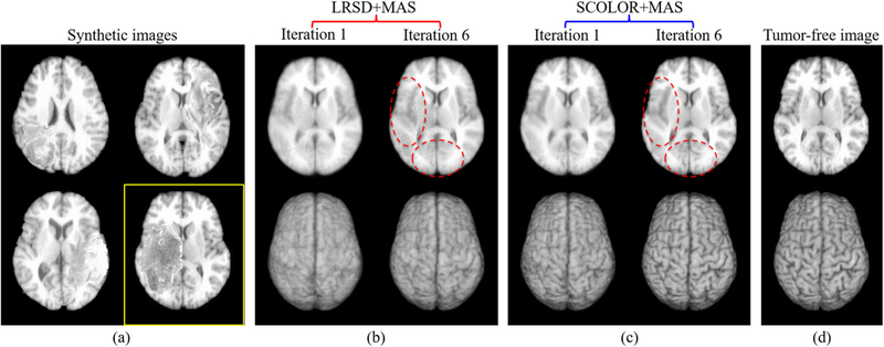
Atlases and synthetic MR tumor brain images are based on a public image dataset called LPBA40 [28], which contains 40 T1-weighted MR normal brain images. Each brain image in LPBA40 has a corresponding label image, which consists of 54 manually segmented brain regions. In each test, we select one image from LPBA40 to generate the synthetic tumor brain image, and the rest 39 images are used as the atlases. The synthetic tumor brain image is generated by inserting tumor(s) derived from a real T1-weighted tumor brain image in BRATS2015. Since all the images from LPBA40 and BRATS2015 are aligned with MNI152 (182×218×182 voxels, 1 × 1 × 1 mm³ voxel size) by affine transformation at the preprocessing stage, we can simply use the image content of the tumor(s) in the real tumor brain image from BRATS2015 to replace the image content at the same location in the selected image from LPBA40. Furthermore, the pressure of the tumor(s) to the surrounding normal tissues is also considered and simulated by adding deformation fields at the boundaries of the tumor(s) (with perpendicular directions to the tumor boundaries and diffused by a Gaussian kernel with σ=3.0) to deform the surrounding normal tissues. The magnitudes of the resulting deformation vectors at the boundary of the inserted tumor(s) are around 3 mm. In this way, 40 synthetic tumor brain images in total are generated in our experiments, each of which contains tumor(s) from different real tumor brain image in BRATS2015. The average proportion (with standard deviation) that the 40 inserted tumor volumes take in the corresponding whole-brain volumes is 0.086±0.053. Some examples of the synthetic brain images are shown in Fig. 4 (a). For each synthetic tumor brain image, we know its tumor-free brain image and the ground truth of manually-segmented brain regions. So the quality of recovered images and the accuracy of segmentation result can be quantified. Specifically, we use recovery error ratio E_rc to quantify the quality of recovered images, which is defined as $E_{rc}=\frac{{\Sigma }_{x\in \Omega }|\widehat{I}\left(x\right)-I^{tf}\left(x\right)|}{{\Sigma }_{x\in \Omega }\left|I^{tf}\left(x\right)\right|}$, where Ω stands for the whole image, and Î and I^tf(x) are image intensities at x of the recovered image and the tumor-free image, respectively. Dice index [29] is used to measure the overlap between the segmented brain regions and the ground truth.

Fig. 4.

Examples of synthetic tumor brain images (a) and the corresponding recovered images of a synthetic image in a yellow rectangle after the 1^st and 6^th iteration of LRSD+MAS (b) and SCOLOR+MAS (c). The corresponding ground truth of tumor-free image is shown in (d). For each recovered image shown at the top row of (b-c), its corresponding 3D rendering is also shown in the bottom row. The recovered images using SCOLOR+MAS are of higher quality for the recovered tumor regions and also have better preservation of normal brain regions than LRSD, especially in the regions marked by red dashed ellipses.

For all the synthetic tumor brain images, LRSD+MAS and SCOLOR+MAS converge after no more than 6 and 4 iterations, respectively. Figs. 4 (b) and (c) show the corresponding recovered images of the synthetic tumor brain image shown in a yellow rectangle of Fig. 4 (a) after the first and last iteration (i.e., the 6^th iteration) of LRSD+MAS and SCOLOR+MAS. As the iteration increases, inter-subject variation of the atlases and the synthetic tumor brain image is reduced by image registration, making the brain anatomical structures clearer in the recovered images of LRSD+MAS and SCOLOR+MAS. Due to spatial constraint in SCOLOR, the recovered tumor region is of higher quality and with also better preservation of normal brain regions than LRSD, as can be observed in Fig. 4 (b) and (c), especially in the regions marked by the red dashed ellipses and 3D renderings shown in the bottom row.

Boxplot of the recovery error ratios of 40 synthetic tumor brain images after each iteration is presented in Fig. 5 (a). The recovery error ratios of both SCOLOR+MAS and LRSD+MAS are decreased after each iteration because of the reduced inter-subject variation between the aligned atlases and the synthetic tumor brain image. Due to the spatial constraint, the recovery error ratios of all the synthetic images in SCOLOR+MAS are much lower than those in LRSD+MAS after the same number of iteration.

Fig. 5.

(a) boxplot of the recovery error ratios of 40 synthetic tumor brain images after each iteration of LRSD+MAS and SCOLOR+MAS, respectively; (b) the spatial constraint C in each iteration; (c) examples of the absolute residual errors of 2 synthetic tumor brain images in the final iteration of LRSD+MAS and SCOLOR+MAS, respectively.

For SCOLOR+MAS, the reduced inter-subject variation can also improve the spatial constraint C in SCOLOR as discussed in Section II.C. Fig. 5 (b) gives some examples of the spatial constraint C for the synthetic tumor brain image shown in the first row of Fig. 5 (c). As can be seen from Fig. 5 (b), some normal brain regions, which are misclassified as tumor regions in the spatial constraint C, are gradually corrected in the subsequent iterations. Moreover, in our experiment, morphological opening operation with the structuring element of a 3D ball (3 voxels radius) is used as post-processing to refine the spatial constraint C. Therefore, two small tumor regions (misclassified) of C in Iter. 4–6 shown in Fig. 5 (b) can be removed by the morphological opening operation.

An intuitive view of the absolute residual errors of two synthetic tumor brain images in the final iteration of LRSD+MAS and SCOLOR+MAS are given in Fig. 5 (c). Clearly, in SCOLOR+MAS, most of the large absolute residual errors are concentrated in the tumor regions, and the absolute residual error is restricted within the normal brain regions. In LRSD+MAS, by contrast, the absolute residual errors in normal brain regions are relatively larger than SCOLOR+MAS.

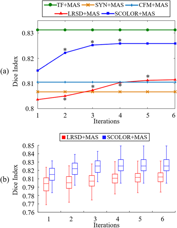
For each synthetic tumor brain image, the Dice indices of the whole-brain and the 54 brain regions between the segmentation results and the ground truth are calculated. Fig. 6 (a) shows the average whole-brain Dice index of 40 segmented synthetic tumor brain images after each iteration of LRSD+MAS and SCOLOR+MAS, and CFM+MAS, respectively. Asterisks marked on the curves of LRSD+MAS and SCOLOR+MAS mean that the Dice indices of current iteration are better than the previous iteration with statistical significance (p<0.05 of Wilcoxon signed rank test [30] over 40 whole-brain Dice indices). In addition, the average whole-brain Dice indices of the segmentation results using the conventional MAS framework (without low-rank based image recovery) on the synthetic tumor brain images (SYN+MAS) and the original tumor-free images of LPBA40 (TF+MAS) are also presented in Fig. 6 (a). Because of the seriously distorted normal brain regions in the recovered images using LRSD, the average whole-brain Dice index after two iterations in LRSD+MAS is even lower than that of SYN+MAS. As the atlases get more aligned to the synthetic tumor brain image after each iteration of LRSD+MAS, the distortion of normal brain regions is suppressed in the recovered image, and the average whole-brain Dice index of LRSD+MAS gets better than SYN+MAS after the third iteration. SCOLOR+MAS converges relatively faster than LRSD+MAS, because the recovered images of SCOLOR+MAS are much closer to the original tumor-free images. Particularly, for most synthetic tumor brain images, SCOLOR+MAS converges after 3–4 iterations, while 4–6 iterations are required in LRSD+MAS. The average whole-brain Dice indices and the standard deviations of the final segmentation results are 0.831±0.010 (TF+MAS), 0.804±0.010 (SYN+MAS), 0.811±0.014 (CFM+MAS), 0.811±0.010 (LRSD+MAS) and 0.826±0.009 (SCOLOR+MAS). Except TF+MAS, the whole-brain Dice indices of SCOLOR+MAS are better than the other methods with statistical significance (p<0.05, Wilconxon signed rank test over 40 whole-brain Dice indices). Fig. 6 (b) shows the boxplot of the whole-brain Dice indices of 40 segmented synthetic tumor brain images after each iteration of LRSD+MAS and SCOLOR+MAS, respectively. Wilcoxon signed rank test is used to test the statistical significance over the 40 whole-brain Dice indices of LRSD+MAS and SCOLOR+MAS after each iteration. The p value for each iteration is 2.425 × 10⁻⁸, indicating that SCOLOR+MAS achieves more accurate segmentation result than LRSD+MAS with statistical significance after each iteration.

Fig. 6.

(a) Average whole-brain Dice indices of 40 segmented synthetic tumor brain images after each iteration of all the methods under comparison; (b) Boxplot of whole-brain Dice indices after each iteration of LRSD+MAS and SCOLOR+MAS, respectively. Since TF+MAS, SYN+MAS and CFM+MAS are not using iterative procedure, their Dice indices are constant. Asterisks marked on the curves of LRSD+MAS and SCOLOR+MAS in (a) mean the whole-brain Dice indices of the current iteration are better than the previous iteration with statistical significance (p<0.05 of Wilcoxon signed rank test).

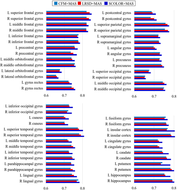
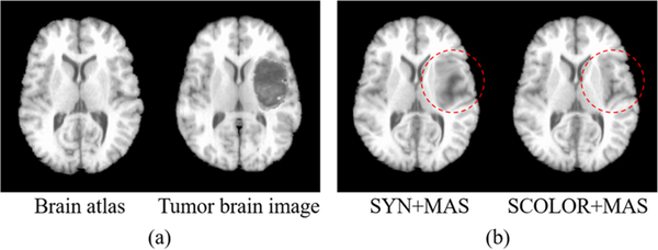
Average brain region Dice indices of the segmentation results by CFM+MAS, LRSD+MAS and SCOLOR+MAS are shown in Fig. 7, and it is evident that our method (SCOLOR+MAS) outperforms CFM+MAS and LRSD+MAS on all the 54 brain regions. Fig. 8 gives an intuitive view of the effect of tumors on registration. A brain atlas shown in the left of Fig. 8 (a) is registered to a tumor brain image shown in the right of Fig. 8 (a) using ORI+MAS (i.e., with tumor) and SCOLOR+MAS, respectively. Due to the presence of a tumor, the registered brain atlas using ORI+MAS is distorted by the tumor as marked by the red dashed circle in the left of Fig. 8 (b). Because of using the recovered tumor region in SCOLOR+MAS, the resulting registered brain atlas is not affected by such distortion. Particularly, the Dice indices of the right insula and the right putamen (both near to the tumor) between the registered brain atlas and the ground truth are (0.424, 0.322) for ORI+MAS and (0.728, 0.604) for SCOLOR+MAS.

Fig. 7.

Average Dice indices of 54 brain regions of 40 segmented synthetic tumor brain images using CFM+MAS, LRSD+MAS (final iteration) and SCOLOR+MAS (final iteration).

Fig. 8.

(a) Examples of a brain atlas and a tumor brain image; (b) Registration results of the brain atlas to the tumor brain image using ORI+MAS and SCOLOR+MAS. The registered brain atlas using ORI+MAS has distorted regions caused by the tumor (marked by red dashed circle), which is not the case for SCOLOR+MAS.

C. Evaluation on real MR tumor brain images

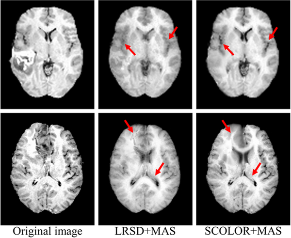
For efficiency, 30 T1-weighted MR tumor brain images are randomly selected from the BRATS2015 dataset [31]. Two images are excluded due to their low image quality, resulting in a total of 28 testing images (as listed in the supplement). Each remaining image contains at least one brain tumor. The average tumor-to-brain volume ratio (± standard deviation) is 0.059±0.037, which covers the size range of most tumors in BRATS2015. The atlases used in LRSD+MAS and SCOLOR+MAS are the 40 normal brain images from LPBA40. Due to the non-existence of tumor-free images, the image recovery error ratio used previously in the evaluation of synthetic images cannot be calculated. In our experiment, the visual quality of the recovered images obtained by SCOLOR+MAS is better than LRSD+MAS, with some examples of the recovered images shown in Fig. 9. It can be observed that the tumor regions are more effectively recovered by SCOLOR+MAS without seriously distorting the normal brain regions as compared to LRSD+MAS, especially in the regions indicated by red arrows.

Fig. 9.

Examples of the recovered images obtained by LRSD+MAS and SCOLOR+MAS, respectively. The recovered images of SCOLOR+MAS exhibit better visual quality than those of LRSD+MAS, especially in the regions indicated by red arrows.

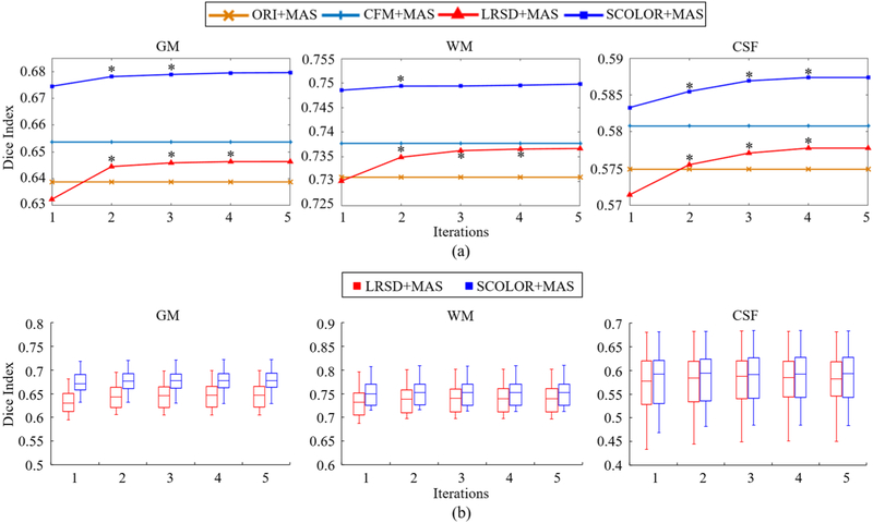
Segmentation accuracy is evaluated by Dice indices of Grey Matter (GM), White Matter (WM), and Cerebrospinal Fluid (CSF) between the segmentation result and the ground truth. Specifically, we use SPM12 [32] to segment GM, WM, and CSF of the 28 testing images and the 40 atlases. These segmentation results are further manually corrected by an expert and regarded as the ground truth. Segmentation results of 28 testing images using conventional MAS framework (without low-rank based image recovery) are also evaluated (denoted by ORI+MAS). It is worth noting that, in the evaluation of segmentation result, all GM, WM and CSF within the tumor regions are ignored in the calculation of Dice index. Fig. 10 (a) shows the average Dice indices of GM, WM and CSF of the 28 testing images after each iteration of ORI+MAS, CFM+MAS, LRSD+MAS and SCOLOR+MAS. For all the 28 images, LRSD+MAS and SCOLOR+MAS converge after no more than 5 and 4 iterations, respectively. In our experiment, the performance of LRSD+MAS in terms of Dice indices of GM, WM and CSF is worse than ORI+MAS after the first iteration. However, as the alignment between the atlases and each tumor brain image gets better, the quality of each resulting recovered image is enhanced, thereby improving the segmentation accuracy. Thus, after the second iteration, LRSD+MAS improves substantially compared with ORI+MAS. Our method achieves the highest Dice indices for GM, WM and CSF. Fig. 10 (b) shows the boxplot of the Dice indices of GM, WM and CSF of LRSD+MAS and SCOLOR+MAS after each iteration.

Fig. 10.

(a) Average Dice indices of GM, WM and CSF of segmented 28 real tumor brain images after each iteration in ORI+MAS, CFM+MAS, LRSD+MAS and SCOLOR+MAS. Since CFM+MAS and ORI+MAS are not using iterative procedure, their average Dice indices of GM, WM and CSF are constant. Asterisks marked on the LRSD+MAS and SCOLOR+MAS curves mean that the Dice indices of GM, WM or CSF of current iteration are better than the previous iteration with statistical significance (p<0.05 of Wilcoxon signed rank test over 28 average Dice indices of GM, WM and CSF); (b) Boxplot of Dice indices of GM, WM and CSF after each iteration of LRSD+MAS and SCOLOR+MAS, respectively

Average Dice indices and standard deviations of the final segmentation results obtained by ORI+MAS, CFM+MAS, LRSD+MAS and SCOLOR+MAS are shown in Table I. The results (Dice indices of GM, WM, and CSF of the 28 testing images for each method) are subject to Wilcoxon signed rank test with significance level of 0.05, which confirms that our method achieves more accurate segmentation result with statistical significance in GM and WM as compared to the other three methods.

TABLE I.

AVERAGE DICE INDICES AND STANDARD DEVIATIONS OF THE FINAL SEGMENTATION RESULTS OBTAINED BY ORI+MAS, LRSD+MAS AND SCOLOR+MAS, RESPECTIVELY.

	GM	WM	CSF
ORI+MAS	0.639±0.024	0.731±0.022	0.575±0.053
CFM+MAS	0.654±0.021	0.738±0.021	0.581±0.051
LRSD+MAS	0.646±0.027	0.736±0.026	0.578±0.059
SCOLOR+MAS	0.679±0.024*	0.750±0.024*	0.587±0.055

^*INDICATES OUR METHOD IS BETTER THAN THE OTHER THREE METHODS (P<0.05).

D. Impact of the number of brain atlases on SCOLOR+MAS

We separately use the 40 synthetic and 28 real tumor brain images to evaluate the impact of the number of adopted brain atlases on SCOLOR+MAS. Specifically, different number of brain atlases, i.e., 5, 10, 15, 20, 25, 30, 35 and 40, is used. It is worth noting that, for the synthetic tumor brain images, one image is selected from LPBA40 to create the synthetic tumor brain image, and the rest are used as atlases. Therefore, at most, 39 atlases instead of 40 atlases can be used for synthtetic tumor brain images. For each number of atlases, we calculate the whole-brain Dice indices for the segmented synthetic images while Dice indices of GM, WM, and CSF for the segmented real images. Fig. 11 shows the boxplot of Dice indices using different numbers of brain atlases. As the number of atlases increases, the segmentation results of both synthetic and real images are improved. Specifically, the improvement of average whole-brain Dice index of the 40 segmented synthetic images using 5 and 39 atlases is 0.804±0.012 to 0.826±0.009, and the improvements of average Dice indices of GM, WM, and CSF of the 28 segmented real images using 5 and 40 atlases are 0.661±0.023 to 0.679±0.024, 0.726±0.023 to 0.750±0.024 and 0.55±0.055 to 0.587±0.055, respectively. It is clear that the use of more brain atalses could get better segmentation result. Table II shows the segmentation accuracy in relation to the number of atlases. Specifically, we show the improvement of the average Dice index between consecutive increase in the number of atlases. We perform Wilcoxon signed rank test over the 40 whole-brain Dice indices (synthetic images) and 28 Dice indices of GM, WM and CSF (real images) between consecutive increase in the number of atlases to get the corresponding p values, respectively. For synthetic images, improvements beyond 20 atlases are statistically significant, but the increase in average Dice index is small (0.001). For real images, improvements for more than 25 atlases are statistically significant, but negligible.

Fig. 11.

Boxplot of Dice indices of whole-brain of segmented 40 synthetic tumor brain images (a), and GM, WM and CSF of segmented 28 real tumor brain images (b) using different number of atlases in SCOLOR+MAS.

TABLE II.

IMPROVEMENT OF SEGMENTATION RESULTS USING DIFFERENT NUMBERS OF ATLASES. THE IMPROVEMENT OF AVERAGE DICE INDEX BETWEEN CONSECUTIVELY INCREASED NUMBER OF ATLASES AND THE CORRESPONDING P VALUE OF WILCOXON SIGNED RANK TEST ARE CALCULATED. ASTERISKS IMPLY STATISTICAL SIGNIFICANCE (P < 0.05)

	Number of atlases		5–10	10–15	15–20	20–25	25–30	30–35	35–40
Synthetic image	Improvement of average Dice		0.013	0.004	0.002	0.001	0.001	0.001	0.001
	p value		3.5E–8*	6.5E–8*	8.2E–8*	1.2E–7*	1.2E–4*	1.3E–3*	2.4E–1
Real image	Improvement of agerage Dice	GM	0.010	0.003	0.002	0.002	0.001	<0.0005	<0.0005
		WM	0.015	0.004	0.003	0.001	<0.0005	<0.0005	<0.0005
		CSF	0.015	0.008	0.006	0.004	0.001	0.001	0.001
		GM	3.8E–6*	2.1E–5*	1.4E–4*	3.5E–4*	2.0E–3*	6.5E–2	7.0E–2
	p value	WM	3.8E–6*	1.1E–5*	2.5E–4*	9.6E–4*	1.2E–2*	1.4E–1	2.6E–1
		CSF	3.8E–6*	4.2E–5*	6.8E–5*	1.3E–4*	1.6E–4*	1.5E–2*	3.5E–2*

E. Impact of parameter λ on SCOLOR+MAS

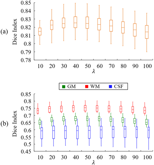
The 40 synthetic and 28 real tumor brain images are separately used as the testing images to evaluate the impact of parameter λ on the segmentation result using SCOLOR+MAS. Specifically, parameter λ is set to values between 10 and 100 (with step size of 10). For different λ, Dice indices of segmentation result are evaluated. Fig. 12 shows the whole-brain Dice indices of the 40 synthetic tumor brain images (Fig. 12 (a)) and the Dice indices of GM, WM and CSF of the 28 real tumor brain images (Fig. 12 (b)) using different λ’s. As λ increases, the Dice indices of segmentation results of both synthetic and real tumor brain images first increase because of the recovery of tumor brain regions and then decrease because of the seriously distorted normal brain regions. However, the performance of SCOLOR+MAS is good and relatively stable using λ from 30 to 60. For example, within the λ range of 30–60, the largest difference of average whole-brain Dice index of segmented synthetic tumor brain images is 0.0019, and the largest differences of average Dice indices of GM, WM and CSF of segmented real tumor brain images are 0.0035, 0.0033 and 0.0007, respectively. Therefore, in our experiment λ is set to 40 in SCOLOR+MAS for both 40 synthetic and 28 real tumor brain images as mentioned before.

Fig. 12.

Boxplot of (a) whole-brain Dice indices of 40 synthetic tumor brain images and (b) Dice indices of GM, WM and CSF of 28 real tumor brain images segmented using SCOLOR+MAS with different λ’s.

F. Impact of parameters a and ß on the spatial constraint

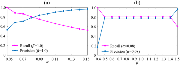
Both the 40 synthetic and 28 real tumor brain images are used together as the testing images to evaluate the impact of parameters α and β on the resulting spatial constraint C, and the evaluation results are shown in Fig. 13. Particularly, for each testing image, C is obtained based on the residual error component (D−B) of the testing image from the final iteration of SCOLOR+MAS. We change α and β separately and calculate the average Recall and Precision [33]. From Fig. 13 (a), we can see that, with increased α, Recall is decreased and Precision is increased. High Recall and Precision indicate good recovery of tumor regions and also preservation of normal brain regions. To set a proper value for α, we have to make a tradeoff between Recall and Precision. Although for tumor regions which are misclassified as normal brain regions in the spatial constraint C can still be recovered by SCOLOR, the recovery strength is relatively weak. In the experiments, we found that, in most cases, the weakly-recovered tumor region can degrade the performance of image registration more than the low-rank induced distorted normal brain region of comparable region size. So we set α to 0.08 (i.e., with Recall being a little bigger than Precision) as mentioned earlier. For β, Recall and Precision of C are stable in a large range of β (Fig. 13 (b)), and β is set to 1.0 as mentioned earlier. Table III lists the average Recall, Precision and Dice indices (α=0.08 and β= 1.0) with standard deviations of calculated spatial constraint C (i.e., detected tumor regions) of the 40 synthetic and 28 real tumor brain images separately.

Fig. 13.

Average Recall and Precision of the resulting spatial constraint C using different values of parameters α (a) and β (b) in SCOLOR+MAS.

TABLE III.

AVERAGE RECALL, PRECISION AND DICE INDEX WITH STANDARD DEVIATION OF THE SPATIAL CONSTRAINT OF SYNTHETIC AND REAL TUMOR BRAIN IMAGES USING α 0.08 AND β 1.0

	Recall	Precision	Dice
Synthetic images	0.832±0.078	0.823±0.091	0.823±0.062
Real images	0.760±0.066	0.724±0.095	0.737±0.057

IV. Discussion and conclusion

We have proposed a new low-rank method, SCOLOR, and integrated it into a new MAS framework, called SCOLOR+MAS, for reliable and accurate segmentation of MR tumor brain images. By introducing a new spatial constraint, SCOLOR+MAS is capable of recovering normal brain appearances from tumor regions while also preserving normal brain structures. This improves atlas registration and eventually segmentation accuracy. We have compared SCOLOR+MAS with 1) LRSD+MAS which uses a conventional low-rank method (LRSD) in the same MAS framework and 2) cost function masking based MAS (CFM+MAS). SCOLOR+MAS outperformed LRSD+MAS in terms of both recovery quality and segmentation accuracy, and CFM+MAS in terms of segmentation accuracy.

One possible application of our method is to improve the accuracy of brain functional connectivity networks (FCN) to do e.g., overall survival time prediction of tumor brain patients. To build the FCN, brain regions are required to be segmented and used to define FCN nodes. If the input image contains tumor(s), the segmentation of brain regions near the tumor(s) will be significantly affected and distorted, making the segmented brain regions inaccurate. Moreover, if the tumor(s) is located near some important brain regions which could be the hubs (i.e., nodes which have connections to many other nodes) in the FCN e.g., the posterior cingulate cortex (PCC), these inaccurately segmented brain regions could result in a seriously distorted FCN. Based on our method, such issue can be solved.

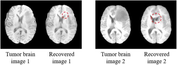
The limitation of our method is that tumor regions should have relatively discriminative appearance from normal brain regions in MR tumor brain images. Otherwise, no tumor regions could be detected and SCOLOR is degraded to a conventional low-rank method. Moreover, tumor mass effects can influence the performance of our method. This is mainly caused by the difficulty in accurately aligning brain atlases based on the highly distorted brain appearance using existing image registration methods. The misalignment can cause artifacts in the recovered images (see Fig. 14).

Fig. 14.

Example of tumor brain images with tumor mass effect and their corresponding recovered images. Due to the misalignment of right lateral ventricles between normal brain atlases and the tumor brain images, artificial structures are generated in the recovered images as marked by the red circles.

In the future, we plan to use more sophisticated methods to do tumor detection to improve the accuracy of the spatial constraint. Moreover, our MAS framework currently can accept just the T1-weighted MR images, since SCOLOR only works well for the input image of the same image modality as the adopted atlases which are T1-weighted MRI. Considering that tumors could be easily detected based on different modalities of MR images e.g., T2-weighted MRI and FLAIR, we plan to improve our MAS framework so that it is able to accept images with different imaging modalities from the T1-weighted MRI atlases.

References

- [1].Wang HZ, Suh JW, Das SR, Pluta JB, Craige C, and Yushkevich PA, “Multi-Atlas Segmentation with Joint Label Fusion,” IEEE transactions on pattern analysis and machine intelligence, vol. 35, pp. 611–623, March 2013. [DOI] [PMC free article] [PubMed] [Google Scholar]
- [2].Awate SP and Whitaker RT, “Multiatlas segmentation as nonparametric regression,” IEEE transactions on medical imaging, vol. 33, pp. 1803–1817, 2014. [DOI] [PMC free article] [PubMed] [Google Scholar]
- [3].Warfield SK, Zou KH, and Wells WM, “Simultaneous truth and performance level estimation (STAPLE): an algorithm for the validation of image segmentation,” IEEE transactions on medical imaging, vol. 23, pp. 903–921, July 2004. [DOI] [PMC free article] [PubMed] [Google Scholar]
- [4].Langerak TR, van der Heide UA, Kotte AN, Viergever MA, Van Vulpen M, and Pluim JP, “Label fusion in atlas-based segmentation using a selective and iterative method for performance level estimation (SIMPLE),” IEEE transactions on medical imaging, vol. 29, pp. 2000–2008, 2010. [DOI] [PubMed] [Google Scholar]
- [5].Sabuncu MR, Yeo BT, Van Leemput K, Fischl B, and Golland P, “A generative model for image segmentation based on label fusion,” IEEE transactions on medical imaging, vol. 29, pp. 1714–1729, 2010. [DOI] [PMC free article] [PubMed] [Google Scholar]
- [6].Sanroma G, Wu G, Gao Y, and Shen D, “Learning to rank atlases for multiple-atlas segmentation,” IEEE transactions on medical imaging, vol. 33, pp. 1939–1953, 2014. [DOI] [PMC free article] [PubMed] [Google Scholar]
- [7].Jia H, Yap P-T, and Shen D, “Iterative multi-atlas-based multi-image segmentation with tree-based registration,” NeuroImage, vol. 59, pp. 422–430, 2012. [DOI] [PMC free article] [PubMed] [Google Scholar]
- [8].Hart MG, Price SJ, and Suckling J, “Connectome analysis for pre-operative brain mapping in neurosurgery,” British journal of neurosurgery, vol. 30, pp. 506–517, 2016. [DOI] [PMC free article] [PubMed] [Google Scholar]
- [9].Yuan W, Wade SL, and Babcock L, “Structural connectivity abnormality in children with acute mild traumatic brain injury using graph theoretical analysis,” Human brain mapping, vol. 36, pp. 779–792, 2015. [DOI] [PMC free article] [PubMed] [Google Scholar]
- [10].Yu Z, Tao L, Qian Z, Wu J, Liu H, Yu Y, Song J, Wang S, and Sun J, “Altered brain anatomical networks and disturbed connection density in brain tumor patients revealed by diffusion tensor tractography,” International journal of computer assisted radiology and surgery, vol. 11, pp. 2007–2019, 2016. [DOI] [PubMed] [Google Scholar]
- [11].Brett M, Leff AP, Rorden C, and Ashburner J, “Spatial normalization of brain images with focal lesions using cost function masking,” NeuroImage, vol. 14, pp. 486–500, 2001. [DOI] [PubMed] [Google Scholar]
- [12].Andersen SM, Rapcsak SZ, and Beeson PM, “Cost function masking during normalization of brains with focal lesions: still a necessity?,” Neuroimage, vol. 53, pp. 78–84, 2010. [DOI] [PMC free article] [PubMed] [Google Scholar]
- [13].Zacharaki EI, Shen D, Mohamed A, and Davatzikos C, “Registration of Brain Images with Tumors: Towards the Construction of Statistical Atlases for Therapy Planning,” in ISBI, Arlington, VA, 2006, pp. 197–200. [Google Scholar]
- [14].Gooya A, Biros G, and Davatzikos C, “Deformable registration of glioma images using EM algorithm and diffusion reaction modeling,” IEEE transactions on medical imaging, vol. 30, pp. 375–390, 2011. [DOI] [PMC free article] [PubMed] [Google Scholar]
- [15].Gooya A, Pohl KM, Bilello M, Cirillo L, Biros G, Melhem ER, and Davatzikos C, “GLISTR: glioma image segmentation and registration,” IEEE transactions on medical imaging, vol. 31, pp. 1941–1954, 2012. [DOI] [PMC free article] [PubMed] [Google Scholar]
- [16].Liu X, Niethammer M, Kwitt R, Singh N, McCormick M, and Aylward S, “Low-rank atlas image analyses in the presence of pathologies,” IEEE transactions on medical imaging, vol. 34, pp. 2583–2591, 2015. [DOI] [PMC free article] [PubMed] [Google Scholar]
- [17].Peng Y, Ganesh A, Wright J, Xu W, and Ma Y, “RASL: Robust alignment by sparse and low-rank decomposition for linearly correlated images,” IEEE transactions on pattern analysis and machine intelligence, vol. 34, pp. 2233–2246, 2012. [DOI] [PubMed] [Google Scholar]
- [18].Evans A, Collins D, and Milner B, “An MRI-based stereotactic brain atlas from 300 young normal subjects, 408, Anaheim,” in Proceedings of the 22nd symposium of the society for neuroscience, 1992. [Google Scholar]
- [19].Gonzalez RC and Woods RE, “Digital image processing prentice hall,” Upper Saddle River , NJ, 2002. [Google Scholar]
- [20].Zhou X, Yang C, and Yu W, “Moving object detection by detecting contiguous outliers in the low-rank representation,” IEEE transactions on pattern analysis and machine intelligence, vol. 35, pp. 597–610, 2013. [DOI] [PubMed] [Google Scholar]
- [21].Liu X, Niethammer M, Kwitt R, McCormick M, and Aylward S, “Low-rank to the rescue-atlas-based analyses in the presence of pathologies,” in International Conference on Medical Image Computing and Computer-Assisted Intervention, 2014, pp. 97–104. [DOI] [PMC free article] [PubMed] [Google Scholar]
- [22].Mazumder R, Hastie T, and Tibshirani R, “Spectral regularization algorithms for learning large incomplete matrices,” Journal of machine learning research, vol. 11, pp. 2287–2322, 2010. [PMC free article] [PubMed] [Google Scholar]
- [23].Boykov Y, Veksler O, and Zabih R, “Fast approximate energy minimization via graph cuts,” IEEE transactions on pattern analysis and machine intelligence, vol. 23, pp. 1222–1239, 2001. [Google Scholar]
- [24].Vercauteren T, Pennec X, Perchant A, and Ayache N, “Non-parametric diffeomorphic image registration with the demons algorithm,” Medical Image Computing and Computer-Assisted Intervention—MICCAI 2007, pp. 319–326, 2007. [DOI] [PubMed] [Google Scholar]
- [25].Aljabar P, Heckemann R, Hammers A, Hajnal JV, and Rueckert D, “Classifier selection strategies for label fusion using large atlas databases,” in International Conference on Medical Image Computing and Computer-Assisted Intervention, 2007, pp. 523–531. [DOI] [PubMed] [Google Scholar]
- [26].Tang Z and Fan Y, “Groupwise image registration guided by a dynamic digraph of images,” Neuroinformatics, vol. 14, pp. 131–145, 2016. [DOI] [PubMed] [Google Scholar]
- [27].Dong W, Shi G, Li X, Ma Y, and Huang F, “Compressive sensing via nonlocal low-rank regularization,” IEEE Transactions on image processing, vol. 23, pp. 3618–3632, 2014. [DOI] [PubMed] [Google Scholar]
- [28].Shattuck DW, Mirza M, Adisetiyo V, Hojatkashani C, Salamon G, Narr KL, Poldrack RA, Bilder RM, and Toga AW, “Construction of a 3D probabilistic atlas of human cortical structures,” NeuroImage, vol. 39, pp. 1064–1080, 2008. [DOI] [PMC free article] [PubMed] [Google Scholar]
- [29].Dice LR, “Measures of the Amount of Ecologic Association Between Species,” Ecology, vol. 26, pp. 297–302, 1945. [Google Scholar]
- [30].Woolson R, “Wilcoxon Signed - Rank Test,” Wiley encyclopedia of clinical trials, 2008. [Google Scholar]
- [31].Menze BH, Jakab A, Bauer S, Kalpathy-Cramer J, Farahani K, Kirby J, Burren Y, Porz N, Slotboom J, and Wiest R, “The multimodal brain tumor image segmentation benchmark (BRATS),” IEEE transactions on medical imaging, vol. 34, pp. 1993–2024, 2015. [DOI] [PMC free article] [PubMed] [Google Scholar]
- [32].Penny WD, Friston KJ, Ashburner JT, Kiebel SJ, and Nichols TE, Statistical parametric mapping: the analysis of functional brain images: Academic press, 2011.
- [33].Powers DM, “Evaluation: from precision, recall and F-measure to ROC, informedness, markedness and correlation,” 2011.