

Abstract
Spectral counting is a straightforward label-free quantitation strategy used in bottom-up proteomics workflows. The application of spectral counting in label-free top-down proteomics workflows can be similarly straightforward but has not been applied as widely as quantitation by chromatographic peak areas or peak intensities. In this study, we evaluate spectral counting for quantitative comparisons in label-free top down proteomics workflows by comparison with chromatographic peak areas and intensities. We tested these quantitation approaches by spiking standard proteins into a complex protein background and comparing relative quantitation by spectral counts with normalized chromatographic peak areas and peak intensities from deconvoluted extracted ion chromatograms of the spiked proteins. Ratio estimates and statistical significance of differential abundance from each quantitation technique are evaluated against the expected ratios and each other. In this experiment, spectral counting was able to detect differential abundance of spiked proteins for expected ratios ≥2, with comparable or higher sensitivity than normalized areas and intensities. We also found that while ratio estimates using peak areas and intensities are usually more accurate, the spectral-counting-based estimates are not substantially worse. Following the evaluation and comparison of these label-free top down quantitation strategies using spiked proteins, spectral counting, along with normalized chromatographic peak areas and intensities, were used to analyze the complex protein cargo of exosomes shed by myeloid-derived suppressor cells collected under high and low conditions of inflammation, revealing statistically significant differences in abundance for several proteoforms, including the active pro-inflammatory proteins S100A8 and S100A9.
Graphical Abstract
Top-down proteomics entails the study of intact proteins by mass spectrometry (MS), an approach that has seen increased adoption as instruments with the necessary high mass resolution become more readily available.1 In recent years, there have been significant advances in top-down proteomics informatics software, providing rapid, automated preprocessing of complex high-resolution protein fragmentation spectra and statistically significant intact protein identification by protein sequence database search. Furthermore, these tools facilitate the characterization of post-translational modifications (PTMs) and single amino acid polymorphisms not provided by the protein sequence database. Currently available commercial tools include ProSightPC,2 while open-source tools such as MashSuite3,4 and TopPIC5 are also available. Hence, intact protein identification and, often, proteoform characterization are now easily attainable. The identification and quantitation of proteoforms by bottom-up proteomics is most times not feasible. After protein digestion, PTM information is often lost due to low sequence coverage and, when more than one PTM is present, it is impossible to determine if the PTMs observed are coming from one or more forms of the same protein, and how they are related.1,6 Proteins and their post-translational modifications regulate protein function, cellular location, and protein−protein interactions. Hence, differential relative quantitation of identified proteoforms by top-down mass spectrometry is needed to elucidate complex cellular processes.
Many of the stable-isotope labeling and label-free quantitation strategies of bottom-up proteomics have been extended for top-down analysis. In the case of label-based quantitation, in vitro incorporation of heavy labels such as 15N-labeling has been successfully performed for quantitation of intact proteins in yeast,7 and stable isotope labeling by amino acids in cell culture (SILAC) has been demonstrated for a 28 kDa standard protein8 and human embryonic stem cell lysates.9 However, metabolic labeling is limited to in vitro cell and tissue culture studies and in vivo animal models.10Tandem mass tag (TMT) labeling was evaluated for top-down proteomics using standard proteins of increasing mass.11 Successful top-down quantitation by stable-isotope labeling is highly dependent on labeling efficiency, reproducibility of sample treatment, reliable precursor isolation, and reproducibility of chromatographic separation. Furthermore, stable-isotope labeling techniques add significant expense to the analysis.
Label-free quantitation in top-down proteomics workflows is usually derived from integrated peak areas or peak intensities of extracted ion chromatograms of full-scan spectra (MS1). Mazur et al. determined differences in the abundance of human apolipoproteins using the peak areas of precursor (m/z) extracted ion chromatograms.12 Phosphorylated proteoform abundance has been measured using peak intensities of the top 5 isotopomers;13 or the most intense isotopic peak14 normalized by the total intensity of all the observed proteoforms. Wu et al. compared the abundance of human saliva proteins from the parotid gland and submandibular/ sublingual gland using the sum of extracted ion chromatogram peak areas of a proteoform’s charge states normalized by the total ion intensity.15 Recent studies reported the use of deisotoped precursor intensities normalized by total ion chromatogram intensity for top-down comparative analysis of complex samples.16–19 These techniques are known to provide good accuracy, but they are currently limited by the time-consuming data processing required, particularly spectra deconvolution and/or integration, as software tools for automated chromatographic-peak-based quantitation analysis are not readily available.
Spectral counting is a label-free quantitation approach, widely used in bottom-up proteomics, that has not yet found significant adoption in top-down proteomics workflows. Quantitation by spectral counting is based on the principle that the likelihood, and repetition, of data-dependent precursor ion selection is higher for abundant precursor ions, and the principle that abundant precursors, if selected for fragmentation, are more likely to result in a successful identification. Together, these suggest that the number of successful peptide identifications from a protein will be correlated with its abundance.20–23 Protein quantitation by peptide spectral counting is simple and straightforward to perform, without the need for additional sample preparation or additional data processing, as the number of peptide identifications from a protein can be easily estimated from the results provided by peptide identification database search engines. While straight-forward, protein quantitation by peptide spectral counting has been shown to result in less accurate estimates of protein relative abundance ratios, when compared to other bottom-up quantitation techniques.24,25
Exosomes are membrane-bound extracellular vesicles of 30 to 100 nm in diameter, which have been reported to carry proteins, lipids, mRNA, and miRNA.26,27 Myeloid-derived suppressor cells (MDSCs) are immune suppressive cells present in virtually all cancer patients. They promote tumor growth by inhibiting antitumor immunity. MDSC shed exosomes,28 and we have reported that exosomes from murine MDSC mediate some MDSC functions. Inflammation is known to increase the abundance of MDSC and to increase their suppressive potency.29,30 Our research group has interrogated the protein cargo from MDSC-derived exosomes previously by bottom-up28 and top-down analysis31 and have identified a large number of proteins and proteoforms, including the pro-inflammatory mediators S100A8 and S100A9, which were found to contribute directly to MDSC activity.28,32
In this study, we evaluate spectral counting of top-down proteoform identifications for use in top-down proteomics quantitation. We use spiked standard proteins in complex protein samples to explore the ability of top-down quantitation by spectral counting, normalized peak intensities, and normalized peak areas to detect abundance differences and estimate protein ratios. Following this comparison using spiked samples, top-down spectral counting is applied to the complex protein cargo isolated from MDSC-derived exosomes produced under conventional and heightened inflammation conditions.
MATERIALS AND METHODS
Reagents.
Recombinant human tumor necrosis factor alpha (TNF-α, 17.3 kDa) was obtained from Novoprotein (Summit, NJ). Ribonuclease A from bovine pancreas (RNase, 13.7 kDa) and carbonic anhydrase from bovine erythrocytes (CAH, 29 kDa) were obtained from Sigma-Aldrich (St. Louis, MO). Ammonium bicarbonate, urea, protease inhibitor cocktail, and phosphatase inhibitor cocktails 2 and 3 were also obtained from Sigma-Aldrich. Deacetylation inhibition cocktail was obtained from Santa Cruz Biotechnologies (Dallas, TX). Deionized water was purified using a Milli-Q system from Millipore (Billerica, MA).
Exosomes from Myeloid-Derived Suppressor Cells.
For each preparation, MDSC were harvested from blood extracted from 1 to 3 BALB/c mice injected with 7000 wild-type syngeneic 4T1 or 4T1 expressing interleukin-1β (4T1/IL-1β) mouse mammary carcinoma cells. Harvested populations that were >90% Gr1+CD11b+ cells as assessed by flow cytometry were incubated in serum-free medium overnight (37 °C, 5% CO2) to release the exosomes. Supernatants from these cultures were ultracentrifuged, and the pelleted exosomes were characterized by centrifugation on 0.25M to 2M sucrose gradients, and by transmission electron microscopy.28 Exosomes shed by MDSC harvested from 4T1 mammary carcinoma are denoted “conventional” and exosomes from 4T1/IL-1β mammary carcinoma denoted “inflammatory” throughout.
Exosomes were lysed with a buffer containing 8 M urea, 50 mM ammonium bicarbonate, and protease, phosphatase, and deacetylase inhibitor cocktails. The exosome lysates were subsequently buffer exchanged using 3 kDa molecular weight cutoff filters to reduce the concentration of urea to less than 0.8 mM, before the amount of total protein was determined using a BCA Pierce colorimetric assay. All samples were prepared in solvent A (2.5% ACN: 72.5% H2O, 0.1% formic acid) prior to LC-MS/MS analysis. All animal experiments were approved by UMBC and UMCP Institutional Animal Care and Use Committees. For each inflammatory condition, four biological replicates were injected in triplicate.
Preparation of Spiked Samples.
Eight samples were prepared by spiking an equal amount of exosome lysate (500 ng) with varying amounts of each of three protein standards. For TNF-α and RNase, 1−50 ng was spiked into the exosome lysate, while for CAH, 10−100 ng was used. The amount of each spiked protein standard in the spiked samples was varied within the given range, keeping the total amount of spiked protein and the total amount of protein as shown in Table S1. Spiked samples were injected in triplicate.
Liquid Chromatography Mass Spectrometry.
Lysates were analyzed using an Ultimate 3000 RSLCnano ultra high-performance liquid chromatographer from Dionex (Sunnyvale, CA) coupled to an orbitrap Fusion Lumos mass spectrometer from Thermo Fisher Scientific (Waltham, MA) controlled by Chromaleon Xpress and Xcalibur 2.3 software, respectively. Samples were desalted and concentrated in a PepSwift RP-4H monolith trap (100 μm × 5 mm) and then separated using a ProSwift RP-4H monolith column (200 μm × 25 cm). Spiked samples were loaded into the trap for 5 min at a flow rate of 5 μL/min and subsequently separated using a linear gradient from 5−55% B for 70 min with a flow rate of 1.5 μL/min, where A is a mixture of 2.5% ACN: 97.5% H2O 0.1% formic acid, and B is a mixture of 75% ACN: 25% H2O 0.1% formic acid. Similarly, exosome samples were loaded for 10 min and subsequently separated using a linear gradient from 1−55% B for 145 min. The column oven and autosampler temperatures were set to 35 and 4 °C, respectively.
The mass spectrometer was configured for intact protein analysis with ion routing multipole pressure of 3 mTorr. Precursor and product ions were analyzed in the Orbitrap with mass resolution 120 000. Precursor ions were selected for fragmentation by “top-speed” data-dependent acquisition in which the top n most abundant precursors are isolated by the quadrupole (using a 1 m/z isolation window) in a fixed 10 s duty cycle. Only precursor ions with a charge state +5 or higher or undetermined charge-state were selected for fragmentation. Dynamic exclusion parameters were optimized using the spiked samples. For the exosome analysis, precursors were excluded for 60 s after being selected. Two fragmentation techniques were used: (1) EThcD with 6 ms reaction time for electron transfer dissociation (ETD) and 10% supplemental higher collision energy (HCD), and (2) 25% normalized collision energy collision induced dissociation (CID). Automatic gain control was set to 1 × 10⁶ for precursor ions and 5 × 10⁵ for fragment ions, with 200 ms maximum injection time. Acquired MS1 and MS2 spectra were the result of averaging 2 microscans for exosome samples and 5 microscans for spiked samples.
Bioinformatics.
Data analysis was performed using the ProSightPD node 1.0 in Proteome Discoverer 2.1 against the mouse database (Uniprot KnowledgeBase, Oct 2015) and a decoy database of reversed protein sequences. Amino-acid sequences for the spiked protein standards were manually added to the mouse database. ProSightPD parameters allowed a precursor mass delta of 2.5 kDa, in order to match post-translationally modified proteins, and a fragment mass delta of 15 ppm. Protein/proteoform spectrum matches (PrSM) were filtered at E-value 10−5, and the false discovery rate (FDR) was estimated to be ≤1%.
The number of PrSMs for each proteoform identified and the total number of PrSMs were counted using an in-house script and verified manually. Signal intensities and areas from deconvoluted extracted ion chromatograms were obtained manually for each proteoform using Xcalibur and normalized by total ion current chromatogram max intensity and total area, respectively.
For spiking experiments, protein ratios between two samples with known spiked amounts were estimated using spectral counts, normalized intensities, and normalized areas. Fisher’s Exact test was used to determine the statistical significance of differential counts between two samples, and Student’s t-test was used for comparison of means by normalized areas and intensities. For the MDSC-derived exosome analysis, a large imbalance in the total number of spectral counts was observed between conventional and inflammatory samples. To correct for this imbalance, observations were scaled to ensure an overall median protein ratio of 1. For spectral counting, statistical significance of differential corrected spectral counts was estimated using Fisher’s Exact and χ2 tests,33 and a sample-label permutation test with a maximum of 100 000 trials per proteoform. The number of trials was reduced by the application of an early stopping rule34 when the cumulative tail probability estimate was considerably larger than the significance threshold. Significance of differential normalized intensities and areas, after median correction, was estimated using the Mann−Whitney test, which is more robust to the presence of outliers. Throughout, Benjamini−Hochberg35 FDR estimates were used to correct for multiple testing. Statistical analysis was carried out in Excel and/or R.
RESULTS AND DISCUSSION
Dynamic Exclusion Parameters for Spectral Counting.
In spectral counting, the number of MS/MS counts observed will depend on MS1 and MS2 spectra quality, precursor ion sampling likelihood, and fragmentation efficiency, all of which correlate with protein abundance. Dynamic exclusion settings are an important consideration, since they have a significant effect on precursor ion sampling.36 Typically, workflows for intact protein analysis use long dynamic exclusion windows, which aims to increase the variety of precursor ions sampled and the number of distinct proteins and proteoforms identified. For top-down protein quantitation by spectral counting, however, multiple identified spectra per proteoform are required for a meaningful statistical analysis. Hence, shorter dynamic exclusions windows are needed. A variety of parameters for short exclusion windows were tested.
Human TNF-α, CAH and RNase standard protein solutions were prepared and analyzed by top-down LC-MS/MS, with each standard represented by a single proteoform. Fifty nanograms of each protein standard was spiked into an exosome sample. Three dynamic exclusion (DE) settings were tested, in triplicate, using the spiked sample: (1) 200 s after being selected once within a period of 30 s; (2) 60 s after being selected once within a period of 30 s; and (3) 60 s after being selected twice in a period of 30 s. Chromatographic peak widths of 180 s are typical under the described experimental conditions.
The number of PrSMs (n = 3) for each spiked standard protein, with respect to specific DE parameter settings is shown in Figure S1. As expected, shorter dynamic exclusion windows increase the spectral count of the spiked proteins, as various precursor ions (m/z) from the same proteoform can be sampled more than once. In addition, permitting the same precursor to be selected twice before exclusion does not seem to increase spectral counts of spiked proteins. The variability of TNF-α spectral counts is increased due to its coelution with other proteoforms from the exosome background, including S100A9 proteoforms. Spectral counts of at least 3 were consistently observed for TNF-α and RNase. Large proteins, such as CAH (29kDa), are challenging for top-down LC-MS/ MS analysis of complex samples as they have lower signal-to-noise ratios due to inefficient ionization, ion transfer, and lower fragmentation efficiency. Moreover, the detection of larger proteins in complex samples is hampered by ion suppression from other coeluting, more readily ionizable proteins. As such, the modest number of CAH PrSMs is not surprising. PrSMs of five proteoforms from the exosome lysate, which represented 0.2 to 37% of the TIC intensity, were also plotted in Figure S1.
Two aspects of top-down proteomics, in particular, make the successful application of spectral counting difficult. First, the need for high resolution for monoisotopic mass determination limits precursor ion sampling speed; and second, the reduced efficiency of intact protein fragmentation, which reduces the number of statistically significant protein identifications from selected precursor ions. Fortunately, state-of-the-art instruments such as the orbitrap Fusion Lumos, which offers higher acquisition speeds and improved fragmentation capabilities,37 minimizes these issues. In this study, averaging two and five microscans for each MS1 and MS2 spectral acquisition was evaluated with precursor exclusion time of 60 s after one selection in 30 s. A single microscan involves ion injection, storage, and detection. Microscans are generally averaged to increase signal-to-noise ratio, at the expense of number of precursors that can be selected in a fixed 10 s duty cycle. In the workflow presented, the average of 2 microscans provided approximately 7 to 8 MS/MS acquisitions compared to approximately 2 to 4 MS/MS when averaging 5 microscans. Figure S1 shows that the spectral counts of spiked proteins was increased for RNase and other proteoforms present in the exosome lysate when averaging two microscans compared to five. Nevertheless, all DE settings and each microscan strategy showed sufficient spectral counts of spiked proteins for reliable estimation of statistical significance. In the interests of increasing the number of proteoforms characterized and quantitated, the averaging of 2 microscans and dynamic exclusion for 60s after selection was used for the spectra collected to evaluate top-down label-free quantitation approaches and to interrogate MDSC-derived exosome protein cargo.
Evaluation of Top-Down Label-Free Quantitative Approaches.
Label-free quantitation in top-down proteomics is largely performed by chromatographic peak areas or peak intensities. In this section, spiked samples were used to explore the sensitivity, precision, and accuracy of spectral counting in top-down proteomics workflows and to compare its performance with that of peak areas and peak intensities. Eight samples of the exosome lysate were spiked as described in the Materials and Methods section. Each spiked sample was analyzed in triplicate, searched against the Uniprot mouse database (plus the spiked standard proteins) and combined. PrSM counts were counted manually from the ProSightPD search output. Normalized intensities and areas were obtained manually from deconvoluted extracted ion chromatograms with signal-to-noise ratio greater than 3. In most cases, the coefficient of variation of normalized intensities or areas of the spiked protein standards in triplicate injections is less than 25%. The comparison of the three approaches included: (1) linearity between spiked and measured counts/signal, (2) detectability of known protein ratios, and (3) accuracy of protein ratios observed.
PrSMs were counted for each standard and plotted against the spiked amount. As shown in Figure 1, a linear trend, with R2 ranging from 0.66 to 0.83, was observed with increasing counts as the amount added to the sample increased. Fisher’s Exact test with Benjamini−Hochberg correction was used to determine the statistical significance of differential abundance for pairs of triplicate spiked samples with different spiked amounts (Figure 2a). In the case of TNF-α and RNase, spectral counting was able to detect, with adjusted p-values values less than 0.05, differential abundance for known protein ratios greater than or equal to 2. The spectral counts for CAH were relatively small, with differential abundance detected for known ratios greater than or equal to 3. This behavior is expected for CAH as it is a relatively large protein and more difficult to identify in complex samples on the chromatographic time scale. Spectral counting differential abundance adjusted p-values are smaller for proteins with high spectral counts due to the use of Fisher’s Exact and χ2 tests, which treat each PrSM as an independent observation. While we expect these count-based adjusted p-values to overestimate the significance of differential abundance observations, this seems to have the greatest impact on adjusted significance estimates much smaller than 0.05, where differential abundance is not in doubt. Hence, using spectral counting, a total of 18%, 27%, and 63% of known spiked protein ratios ≥2 go undetected for TNF-α, RNase, and CAH, respectively. Pairs of spiked samples with no change for a spiked protein typically did not show a statistically significant differential abundance p-value after multiple test correction, except for TNF-α. These observations are highlighted in Figure 2, in which protein standard comparisons with known spiked protein ratios >2 not detected (by adjusted p-values values less than 0.05) are defined as false negative, and those with known spiked protein ratios <2 that are flagged as differential defined as false positive.
Figure 1.
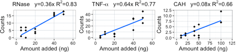
Calibration curve of PrSM counts versus the protein standards amount spiked. A linear relationship was observed for all standards.
Figure 2.
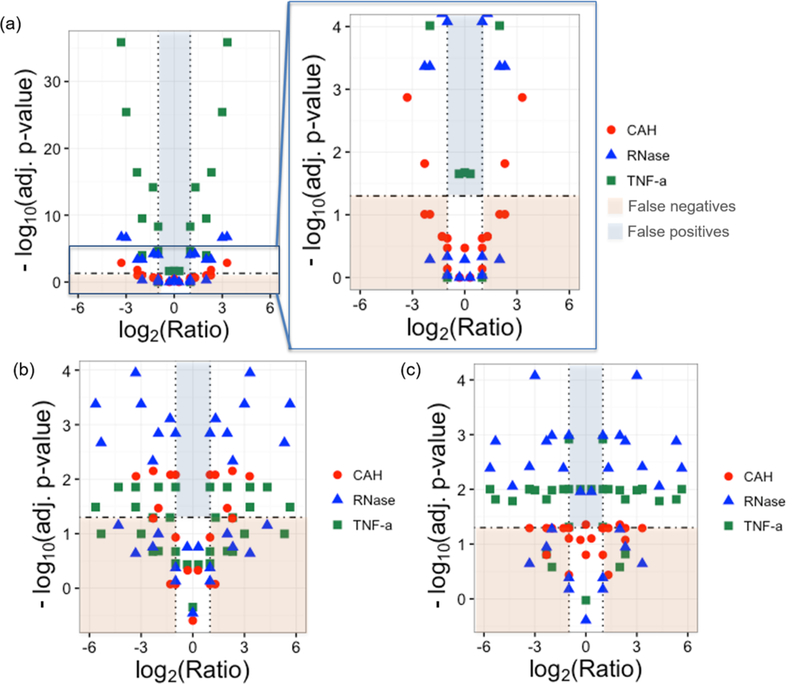
Detectability of abundance differences for (a) spectral counting, (b) normalized intensities, and (c) normalized areas are shown by plotting −log10(adj. p-value) vs expected protein ratio. Note that for spectral counting, an additional plot of scale comparable to plots shown for the other techniques was added. Statistically significant results have a −log10(adj. p-value) ≥ 1.3, which corresponds to an adjusted p-value of 0.05, and it is marked by an horizontal dashed line in the plots. Dotted vertical lines correspond to a 2-fold change in abundance. False positives are highlighted in light blue and are defined as protein standard comparisons with known spiked protein ratios <2 (log2(Ratio) between −1 and 1) and −log10(adj. p-value) ≥ 1.3. False negatives are highlighted in light red and correspond to protein standard with known spiked protein ratios >2 (log2(Ratio) < −1 and log2(Ratio) > 1) and −log10(adj. p-value) ≤ 1.3.
For peak intensities and areas, plots of normalized intensities and normalized areas against the spiked amount were made for each standard, and as expected, a linear relationship was also observed, with R2 ranging from 0.68 to 0.90 (Figure S2). The Student’s t-test with Benjamini−Hochberg correction was used to estimate the statistical significance of differential abundance for pairs of triplicate spiked samples with different spiked amounts. Figure 2b,c show that 50%, 33%, and 36% of known spiked protein ratios ≥2 are not detected, by adjusted p-value less than 0.05, when normalized intensities are used for TNF-α, RNase, and CAH, respectively. When normalized areas are used, 13%, 31%, and 72% of known spiked protein ratios ≥2 go undetected. No false positives were detected by normalized intensities, and normalized areas showed one false positive for TNF-α and RNase. Despite the intrinsically more robust chromatographic peak measurements, there is still considerable variation in the observations, and each acquisition results in just one observation—only the strongest differential signals are significant with just six observations. As such, spectral counting appears to offer comparable or higher detection sensitivity for differential abundance when there are relatively few replicates. It is important to acknowledge that spectral counting, though straightforward to implement, still depends on protein identification of MS2 spectra. Peak areas and intensities, though less sensitive in this context, can be applied to proteins that are not identified, as long as their intact mass (MS1) and retention times is known.
The use of PrSM counts to determine protein ratios was also evaluated, and a weak linear relationship was found between the log2 of observed and expected ratios (Figure S3a). The calculated protein ratios are markedly affected by the variability in PrSM counts with R2 in the 0.34−0.69 range. RNase showed poor linearity due to the high variability of spectral counts at the lower spiking levels. This observation can be explained by competing coeluting proteins that become relatively more abundant as the amount spiked is reduced. Nevertheless, the slope of the regression lines for each standard range from 0.68 to 1.40, around the ideal value of 1.0, suggesting that despite the variation in the estimates, the ratios follow the correct trend. Moreover, protein ratios were also calculated using normalized intensities and areas and plotted against the expected ratios (Figures S3b and S3c). In the case of normalized intensities, a linear trend (R2 0.61−0.90) was observed for all protein standards with slopes ranging from 0.97 to 1.43. Similarly, when normalized areas were used linear trends (R2 0.50−0.66) are observed with slopes ranging from 1.00 to 1.42. Normalized intensities and normalized areas provide somewhat more accurate protein ratio estimates, though quite reasonable estimates seem to be possible by spectral counting, allowing us to assess trends quickly without the need of extra data processing. Note that independent of the approach used, in most cases the protein ratios observed for pairs of spiked samples with no changes are lower than 2 (log2(Ratio) = 1), with an unchanged CAH sample comparison showing spectral counting log2(Ratio) of 1.2 and normalized areas log2(Ratio) of 0.9. Linear regression plots of protein ratios without log2 transformation are shown in Figure S4.
Differential Abundances of MDSC Exosomal Proteins.
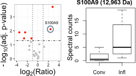
Having demonstrated the feasibility of top-down spectral-counting for detection of differential abundance, we applied the technique to exosomes shed by myeloid-derived suppressor cells collected from tumor-bearing mice with heightened and conventional inflammation. Four biological replicates for each condition were each analyzed in triplicate. For each condition, a total of 12 data files were searched against the Uniprot mouse database and combined. Fifty-two proteoforms, representing 14 distinct proteins, were identified in conventional exosomes. Seventy proteoforms, representing 20 distinct proteins, were identified in inflammatory exosomes. The identified proteins are in agreement with those from our previous top-down analysis of the protein cargo in exosomes from mice with high inflammation31 although fewer identifications are observed in this study as just a single round of chromatographic separation was performed. Three proteins from the S100 protein family were identified: S100A6, S100A8, and S100A9. The low-mass proteins S100A8 and S100A9 are highly abundant pro-inflammatory mediators in MDSC-derived exosomes and have been shown to contribute directly to MDSC activity.28,32 Different proteoforms may have distinct roles in tumor growth and metastasis, so determining the S100A8 and S100A9 proteoforms which show differential abundance when subject to different levels of inflammation is expected to provide unique insight. This study identified a total of 21 and 25 proteoforms from S100A8 in conventional and inflammatory exosomes, respectively. In the case of S100A9, five proteoforms were found; however, only one proteoform (12 963 Da) was observed in both conditions. Regarding PTM assignments, in most cases, our methodology provided good fragmentation density and straightforward characterization (Figure 3). The proportion of residue cleavage obtained by combining the spectra of one precursor fragmented by both EThcD and CID ranged from 13 to 97% depending on the proteoform (Table S2).
Figure 3.
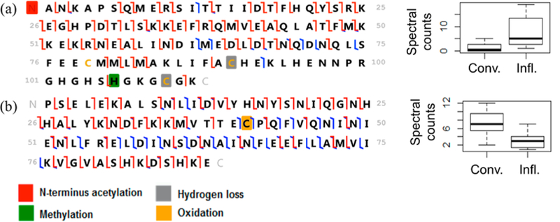
Annotated sequences and spectral counts comparison for (a) S100A9 (12 963 Da) and (b) S100A8 (10 173 Da) proteoforms present in exosomes. High fragmentation density allows simple putative PTMs assignment. Sequences are shown including observed product ions, which are represented in blue (b and y-ions) and red (c and z-ions), and their color-coded putative PTMs.
All PrSMs were counted and summed for each proteoform by inflammation condition. Sampling depth varied between the conditions, with a total of 6434 PrSMs observed from inflammatory exosomes and 2131 PrSMs from conventional exosomes. The observed bias was corrected by scaling down all inflammatory observations to ensure a global median of protein ratios of one.38–41 This approach encodes the prior belief that, absent any systematic bias, most proteoforms are not differentially abundant with log2 ratios of all identified proteoforms distributed symmetrically about zero. Systematic biases, which may occur due to the complexity of biological samples, and unavoidable variation in sample loading, chromatographic separation, proteoform ionization efficiencies, and data-dependent fragmentation with preferential selection for high abundance precursor ions, can be removed by centering the log-ratios about zero. Median normalization was applied separately to spectral counts, peak areas, and peak intensities (Figure S5).
Twenty-two proteoforms identified in at least two biological replicates for each condition were selected for quantitative comparison. For spectral counting, differences in abundance were evaluated using the count-based Fisher’s Exact and χ2 tests, and a sample-label permutation test with a maximum of 100 000 trials for each proteoform. Benjamini−Hochberg FDR estimation was used to correct for multiple testing for each test strategy. We chose to apply a sample-label permutation test to the Fisher’s Exact p-values to provide empirical confirmation of statistical significance by the Fisher’s Exact test, given the nonindependence of spectral counts. In this case, with 12 conventional and 12 inflammatory spectral datafiles, there are sufficient permutations of the sample labels for good empirical p-value estimates. In general, we found that when the differences in spectral counts were consistent across biological and technical replicates within a condition, significant Fisher’s Exact tests were confirmed with significant sample-label permutation tests. However, even when the tests agreed, the sample-label permutation tests were much more conservative than the Fisher’s Exact tests. Differences in normalized areas and intensities were detected using the Mann−Whitney test with Benjamini−Hochberg correction. Table 1 shows the calculated protein ratios and adjusted p-values, with 16 out of the 22 proteoforms showing no statistically significant abundance difference. Proteoform ratio estimates calculated using spectral counts were plotted against proteoform ratio estimates based on peak areas and intensities (Figure S6), showing good correspondence between the estimates from different techniques.
Table 1.
Proteoforms Identified with Estimated Ratios by Spectral Counting and Normalized Intensity and Areaa
| spectral counting |
peak areas |
peak intensities |
||||||
|---|---|---|---|---|---|---|---|---|
| observed mass (Da) |
log2(Ratio) (counts) |
Fisher’s Exact FDR |
perm. sample FDR |
chi-square FDR |
log2(Ratio) (area) |
Mann−Whitney FDR |
log2(Ratio) (intensity) |
Mann−Whitney FDR |
| Q9CPW5: Translocon-associated protein subunit beta | ||||||||
| 16308.28 | −1.6 | 1.4 × 10⁻⁸ | 1.2 × 10⁻¹ | 6.2 × 10⁻⁸ | −2.6 | 1.6 × 10⁻¹ | −2.0 | 4.0 × 10⁻² |
| P62204: Calmodulin | ||||||||
| 16779.85 | −1.6 | 1.1 × 10⁻⁴ | 2.3 × 10⁻¹ | 1.2 × 10⁻⁴ | −2.5 | 1.9 × 10⁻¹ | −1.2 | 7.3 × 10⁻¹ |
| 16795.82 | −1.6 | 5.4 × 10⁻⁴ | 1.2 × 10⁻¹ | 5.6 × 10⁻⁴ | −2.3 | 7.1 × 10⁻¹ | −1.5 | 7.3 × 10⁻¹ |
| P22752: Histone H2A type 1 | ||||||||
| 12354.95 | 1.2 | 7.1 × 10⁻³ | 1.4 × 10⁻¹ | 5.6 × 10⁻³ | 1.3 | 1.2 × 10⁻¹ | 1.4 | 7.5 × 10⁻² |
| P01942: Hemoglobin subunit alpha | ||||||||
| 15063.71 | −0.6 | 1.9 × 10⁻¹ | 6.3 × 10⁻¹ | 1.3 × 10⁻¹ | −1.6 | 3.9 × 10⁻¹ | −1.0 | 4.9 × 10⁻¹ |
| 15077.81 | −0.6 | 2.7 × 10⁻¹ | 6.3 × 10⁻¹ | 2.0 × 10⁻¹ | −1.7 | 3.5 × 10⁻¹ | −0.9 | 5.0 × 10⁻¹ |
| P09602: Nonhistone chromosomal protein HMG-17 | ||||||||
| 9286.02 | 0.1 | 9.2 × 10⁻¹ | 6.8 × 10⁻¹ | 6.8 × 10⁻¹ | 0.0 | 2.1 × 10⁻² | 0.4 | 4.7 × 10⁻² |
| P14069: Protein S100-A6 | ||||||||
| 10074.27 | −0.7 | 1.3 × 10⁻¹ | 2.8 × 10⁻¹ | 9.5 × 10⁻² | 0.0 | 3.1 × 10⁻² | 0.3 | 3.1 × 10⁻² |
| P31725: Protein S100-A9 | ||||||||
| 12963.26 | 2.4 | 3.0 × 10‑12 | 7.5 × 10‑3 | 6.5 × 10‑11 | 4.6 | 5.8 × 10‑4 | 3.8 | 2.9 × 10‑2 |
| P27005: Protein S100-A8 | ||||||||
| 10101.98 | 0.3 | 8.7 × 10⁻¹ | 3.4 × 10⁻¹ | 5.9 × 10⁻¹ | 0.5 | 1.5 × 10⁻² | 1.0 | 2.6 × 10⁻² |
| 10140.03 | 2.8 | 4.8 × 10‑5 | 1.9 × 10‑4 | 7.4 × 10‑5 | 3.0 | 5.1 × 10‑3 | 2.0 | 2.5 × 10‑2 |
| 10157.05 | 0.3 | 1.3 × 10⁻¹⁰ | 9.2 × 10⁻² | 4.4 × 10⁻⁶ | 0.6 | 2.2 × 10⁻³ | 0.0 | 2.5 × 10⁻² |
| 10172.99 | −1.2 | 2.8 × 10‑5 | 3.5 × 10‑2 | 4.1 × 10‑5 | −0.2 | 1.5 × 10‑2 | 1.1 | 2.6 × 10‑2 |
| 10179.05 | 0.1 | 9.7 × 10⁻¹ | 8.8 × 10⁻¹ | 7.7 × 10⁻¹ | 0.2 | 8.0 × 10⁻³ | 0.6 | 2.9 × 10⁻² |
| 10189.07 | −2.6 | 9.9 × 10‑10 | 3.5 × 10‑2 | 7.2 × 10‑9 | −1.4 | 4.7 × 10‑1 | −0.4 | 6.8 × 10‑1 |
| 10205.02 | −3.5 | 3.5 × 10‑7 | 1.3 × 10‑2 | 2.6 × 10‑6 | −2.1 | 7.2 × 10‑1 | −0.6 | 7.5 × 10‑1 |
| 10212.54 | −0.8 | 4.9 × 10⁻¹ | 5.1 × 10⁻¹ | 3.1 × 10⁻¹ | −0.7 | 9.6 × 10⁻¹ | 1.8 | 6.6 × 10⁻¹ |
| 10221.02 | −2.4 | 8.0 × 10‑12 | 1.3 × 10‑2 | 7.6 × 10‑11 | −2.7 | 7.1 × 10‑1 | −2.2 | 7.3 × 10‑1 |
| 10276.01 | −0.4 | 5.1 × 10⁻¹ | 4.1 × 10⁻¹ | 3.6 × 10⁻¹ | 0.0 | 5.2 × 10⁻² | 1.4 | 4.0 × 10⁻² |
| 10288.07 | −0.2 | 4.1 × 10⁻¹ | 5.1 × 10⁻¹ | 3.6 × 10⁻¹ | 1.4 | 5.8 × 10⁻⁴ | 0.2 | 2.5 × 10⁻² |
| 10304.04 | −1.3 | 2.3 × 10⁻⁴ | 6.3 × 10⁻² | 2.5 × 10⁻⁴ | 0.3 | 9.6 × 10⁻³ | −0.4 | 2.4 × 10⁻¹ |
| 10340.04 | 0.0 | 9.7 × 10⁻¹ | 9.4 × 10⁻¹ | 9.8 × 10⁻¹ | 0.3 | 5.8 × 10⁻⁴ | 0.4 | 2.5 × 10⁻² |
Proteoforms found to be differentially abundant by spectral counting shown in bold italics.
Four oxidized proteoforms of S100A8 (P27005:10 173 Da, 10 205 Da, 10 189 Da and 10 221 Da) were found to be 2.3- to 6-fold greater in abundance in conventional exosomes by spectral counting, with sample-label permutation test adjusted p-values of 0.013 to 0.035. Neither normalized peak areas nor intensities were able to detect these abundance differences as statistically significant after multiple test correction. This set of S100A8 proteoforms comprise the loss of M1 and oxidation of C42 to sulfenic acid (P27005; 10 173 Da), sulfinic acid (P27005; 10 189 Da), sulfonic acid (P27005; 10 205 Da), and sulfonic acid with further oxidation of M37 (P27005; 10 221 Da). It has been proposed previously that S100A8 may act as a scavenger of reactive oxygen species during inflammation, offering protection against oxidative damage.42,43 Additionally, Raftery et al. observed that oxidized monomers of S100A8 were produced in vivo in PMA-stimulated neutrophils and that following oxidation their chemotactic activity was maintained.44
Proteoforms of S100A8 (P27005; 10 140 Da) and S100A9 (P31725; 12 963 Da) were found in greater abundance in exosomes collected under inflammatory conditions with strong agreement among all three quantitation approaches. In the case of S100A8 (P27005; 10 140 Da), a mass difference of −148.04 Da is observed, which could be explained by the loss of M1 and (artifactual) loss of ammonia. Due to ineffective precursor isolation between the S100A8 proteoforms of mass 10 140 Da and 10 157 Da, fragmentation is not able to provide full characterization of the loss of ammonia. Based on its fragments, the S100A9 proteoform is characterized by the loss of M1, acetylation of A2, methylation of H107, as previously reported,45 and the presence of a disulfide bond between C91 and C111 (Figure 3).
S100A9 is known to form a heterodimer with S100A8, which plays a role in MDSC immunosuppressive activity. MDSC that develop under heightened inflammation are more suppressive and accumulate in vivo to higher levels as compared to MDSC that develop in less inflammatory environments.46 S100A8/A9 is an established driver of MDSC accumulation and suppressive activity.32 It occurs with greater abundance in the inflammatory MDSC and is responsible for this enhanced MDSC activity.32 In the present work, proteoforms of S100A8 and A9 are also shown to be present in the exosomes shed by MDSC, and the single proteoform of S100A9 that could be analyzed is found to be of higher abundance in inflammatory conditions. These results support the concept that not only MDSC themselves but also MDSC-derived exosomes provide an autocrine feedback mechanism that facilitates tumor progression by enhancing immune suppression. Individual roles for individual proteoforms remain to be explored.
CONCLUSIONS
This study evaluates spectral counting for top-down proteomics quantitation comparisons with respect to normalized chromato-graphic peak areas and intensities. Ratios of spectral counts are evaluated with a variety of statistical tests to ensure sensitive, yet robust, detection of differential abundance. Spiking experiments demonstrate that spectral counting provides comparable or higher sensitivity and robustness as quantification by normalized chromatographic peak intensities or areas. The main advantage of spectral counting is its simplicity, as the search outputs can be used directly to obtain counts with minimum postprocessing analysis. As such, spectral counting may represent a good preliminary screen for putative differentially abundant proteoforms in large studies with many biological and technical replicates. Moreover, protein ratios obtained from spectral counts were found to be in good agreement with proteoform ratios obtained using normalized peak areas and intensities. All three strategies were applied to MDSC-derived exosomes under conventional and heightened inflammation conditions, and differences in abundance were observed for a number of potentially active S100A8 and S100A9 proteoforms.
Supplementary Material
ACKNOWLEDGMENTS
This project was funded by the National Institutes of Health grants GM021248 and OD019938. We thank Virginia Clements for animal husbandry.
Footnotes
Supporting Information
Preparation of spiked samples; effect of dynamic exclusion and microscans averaging on PrSMs counts; calibration curves of normalized area, normalized intensity, and spectral counts vs amount of protein standard spiked; linear regression plots of observed and expected protein ratios without log2 transformation; comparison of expected and observed protein ratios estimated by spectral counting, normalized intensities, and normalized areas; distribution of log2(ratios) estimated using intensities, areas, and spectral counts, before and after normalization; comparison of log2(ratios) found for the 22 quantified proteoforms in the exosome samples (PDF)Complete list of proteoforms identified and comparison of differential abundances calculated by spectral counting, normalized intensities, and areas (XLSX)
Notes
The authors declare no competing financial interest.
REFERENCES
- (1).Perkel JM Science 2015, 349, 1243–1245. [Google Scholar]
- (2).LeDuc RD; Kelleher NL Curr. Protoc. Bioinforma 2007, 19 (Unit 13.6), 1–28. [DOI] [PubMed] [Google Scholar]
- (3).Guner H; Close PL; Cai W; Zhang H; Peng Y; Gregorich ZR; Ge YJ Am. Soc. Mass Spectrom 2014, 25, 464–470. [DOI] [PMC free article] [PubMed] [Google Scholar]
- (4).Cai W; Guner H; Gregorich ZR; Chen AJ; Ayaz-Guner S; Peng Y; Valeja SG; Liu X; Ge Y Mol. Cell. Proteomics 2016, 15, 703–714. [DOI] [PMC free article] [PubMed] [Google Scholar]
- (5).Kou Q; Xun L; Liu X Bioinformatics 2016, 1–3. [DOI] [PMC free article] [PubMed]
- (6).Zhang H; Ge Y Circ.: Cardiovasc. Genet 2011, 4, 711. [DOI] [PMC free article] [PubMed] [Google Scholar]
- (7).Du Y; Parks BA; Sohn S; Kwast KE; Kelleher NL Anal. Chem 2006, 78, 686–694. [DOI] [PubMed] [Google Scholar]
- (8).Waanders LF; Hanke S; Mann MJ Am. Soc. Mass Spectrom 2007, 18, 2058–2064. [DOI] [PubMed] [Google Scholar]
- (9).Collier TS; Sarkar P; Rao B; Muddiman DC J. Am. Soc. Mass Spectrom 2010, 21, 879–889. [DOI] [PubMed] [Google Scholar]
- (10).Mann M Nat. Rev. Mol. Cell Biol 2006, 7, 952–958. [DOI] [PubMed] [Google Scholar]
- (11).Hung CW; Tholey A Anal. Chem 2012, 84, 161–170. [DOI] [PubMed] [Google Scholar]
- (12).Mazur MT; Cardasis HL; Spellman DS; Liaw A; Yates NA; Hendrickson RC Proc. Natl. Acad. Sci. U. S. A 2010, 107, 7728–7733. [DOI] [PMC free article] [PubMed] [Google Scholar]
- (13).Zhang JI; Talaty N; Costa AB; Xia Y; Tao WA; Bell R; Callahan JH; Cooks RG Int. J. Mass Spectrom 2011, 301, 37–44. [Google Scholar]
- (14).Chen Y; Hoover ME; Dang X; Shomo AA; Guan X; Marshall AG; Freitas MA; Young NL Mol. Cell. Proteomics 2016, 15, 818–833. [DOI] [PMC free article] [PubMed] [Google Scholar]
- (15).Wu S; Brown JN; Tolić N; Meng D; Liu X; Zhang H; Zhao R; Moore RJ; Pevzner P; Smith RD; Pasa-Tolic L Proteomics 2014, 14, 1211–1222. [DOI] [PubMed] [Google Scholar]
- (16).Ntai I; Kim K; Fellers RT; Skinner OS; Smith AD; Early BP; Savaryn JP; LeDuc RD; Thomas PM; Kelleher NL Anal. Chem 2014, 86, 4961–4968. [DOI] [PMC free article] [PubMed] [Google Scholar]
- (17).Ntai I; LeDuc RD; Fellers RT; Erdmann-Gilmore P; Davies SR; Rumsey J; Early BP; Thomas PM; Li S; Compton PD; Ellis MJC; Ruggles KV; Fenyö D; Boja ES; Rodriguez H; Townsend RR; Kelleher NL Mol. Cell. Proteomics 2016, 15, 45–56. [DOI] [PMC free article] [PubMed] [Google Scholar]
- (18).Durbin KR; Fornelli L; Fellers RT; Doubleday PF; Narita M; Kelleher NL J. Proteome Res 2016, 15, 976–982. [DOI] [PMC free article] [PubMed] [Google Scholar]
- (19).Savaryn JP; Toby TK; Catherman AD; Fellers RT;LeDuc RD; Thomas PM; Friedewald JJ; Salomon DR; Abecassis MM; Kelleher NL Proteomics 2016, 16, 2048–2058. [DOI] [PMC free article] [PubMed] [Google Scholar]
- (20).Allet N; Barrillat N; Baussant T; Boiteau C; Botti P; Bougueleret L; Budin N; Canet D; Carraud S; Chiappe D; Christmann N; Colinge J; Cusin I; Dafflon N; Depresle B; Fasso I; Frauchiger P; Gaertner H; Gleizes A; Gonzalez-Couto E; Jeandenans C; Karmime A; Kowall T; Lagache S; Mahe E; Masselot A; Mattou H; Moniatte M; Niknejad A; Paolini M; Perret F; Pinaud N; Ranno F; Raimondi S; Reffas S; Regamey P-O; Rey P-A; Rodriguez-Tome P; Rose K; Rossellat G; ´ Saudrais C; Schmidt C; Villain M; Zwahlen C Proteomics 2004, 4, 2333–2351. [DOI] [PubMed] [Google Scholar]
- (21).Old WM; Meyer-Arendt K; Aveline-Wolf L; Pierce KG; Mendoza A; Sevinsky JR; Resing KA; Ahn NG Mol. Cell. Proteomics 2005, 4, 1487–1502. [DOI] [PubMed] [Google Scholar]
- (22).Liu H; Sadygov RG; Yates JR Anal. Chem 2004, 76, 4193–4201. [DOI] [PubMed] [Google Scholar]
- (23).Fu X; Gharib SA; Green PS; Aitken ML; Frazer DA; Park DR; Vaisar T; Heinecke JW J. Proteome Res 2008, 7, 845–854. [DOI] [PubMed] [Google Scholar]
- (24).Bantscheff M; Schirle M; Sweetman G; Rick J; Kuster B Anal. Bioanal. Chem . 2007, 389, 1017–1031. [DOI] [PubMed] [Google Scholar]
- (25).Lundgren DH; Hwang S-I; Wu L; Han DK Expert Rev. Proteomics 2010, 7, 39–53. [DOI] [PubMed] [Google Scholar]
- (26).Gould SJ; Raposo GJ Extracell. Vesicles 2013, 2, 20389. [DOI] [PMC free article] [PubMed] [Google Scholar]
- (27).Raposo G; Stoorvogel WJ Cell Biol 2013, 200, 373–383. [DOI] [PMC free article] [PubMed] [Google Scholar]
- (28).Burke M; Choksawangkarn W; Edwards N; OstrandRosenberg S; Fenselau CJ Proteome Res 2014, 13, 836–843. [DOI] [PMC free article] [PubMed] [Google Scholar]
- (29).Bunt SK; Sinha P; Clements VK; Leips J; OstrandRosenberg SJ Immunol 2006, 176, 284–290. [DOI] [PubMed] [Google Scholar]
- (30).Parker KH; Sinha P; Horn LA; Clements VK; Yang H; Li J; Tracey KJ; Ostrand-Rosenberg S Cancer Res 2014, 74, 5723–5733. [DOI] [PMC free article] [PubMed] [Google Scholar]
- (31).Geis-Asteggiante L; Dhabaria A; Edwards N; OstrandRosenberg S; Fenselau C Int. J. Mass Spectrom 2015, 378, 264–269. [DOI] [PMC free article] [PubMed] [Google Scholar]
- (32).Sinha P; Okoro C; Foell D; Freeze HH; OstrandRosenberg S; Srikrishna GJ Immunol 2008, 181, 4666–4675. [DOI] [PMC free article] [PubMed] [Google Scholar]
- (33).Zhang B; VerBerkmoes NC; Langston MA; Uberbacher E; Hettich RL; Samatova NF J. Proteome Res 2006, 5, 2909–2918. [DOI] [PubMed] [Google Scholar]
- (34).Jiang H; Salzman J Biometrika 2012, 99, 973–980. [DOI] [PMC free article] [PubMed] [Google Scholar]
- (35).Benjamini Y; Hochberg Y J. R. Stat. Soc. B 1995, 57, 289–300. [Google Scholar]
- (36).Zhang Y; Wen Z; Washburn MP; Florens L Anal. Chem 2009, 81, 6317–6326. [DOI] [PubMed] [Google Scholar]
- (37).Eliuk S; Makarov A Annu. Rev. Anal. Chem 2015, 8, 61–80. [DOI] [PubMed] [Google Scholar]
- (38).Quackenbush J Nat. Genet 2002, 32, 496–501. [DOI] [PubMed] [Google Scholar]
- (39).Karpievitch YV; Dabney AR; Smith RD BMC Bioinf 2012, 13 (Suppl 16), S5. [DOI] [PMC free article] [PubMed] [Google Scholar]
- (40).Listgarten J; Emili A Mol. Cell. Proteomics 2005, 4, 419–434. [DOI] [PubMed] [Google Scholar]
- (41).Callister SJ; Barry RC; Adkins JN; Johnson ET; Qian WJ; Webb-Robertson BJM; Smith RD; Lipton MS J. Proteome Res . 2006, 5, 277–286. [DOI] [PMC free article] [PubMed] [Google Scholar]
- (42).Lim SY; Raftery MJ; Goyette J; Hsu K; Geczy CL J. Leukocyte Biol 2009, 86, 577–587. [DOI] [PubMed] [Google Scholar]
- (43).Lim SY; Raftery MJ; Geczy CL Antioxid. Redox Signaling 2011, 15, 2235–2248. [DOI] [PubMed] [Google Scholar]
- (44).Raftery MJ; Yang Z; Valenzuela SM; Geczy CL J. Biol. Chem 2001, 276, 33393–33401. [DOI] [PubMed] [Google Scholar]
- (45).Raftery MJ; Harrison C. a; Alewood P; Jones a; Geczy CL Biochem. J 1996, 316, 285–293. [DOI] [PMC free article] [PubMed] [Google Scholar]
- (46).Bunt SK; Yang L; Sinha P; Clements VK; Leips J; Ostrand-Rosenberg S Cancer Res 2007, 67, 10019–10026. [DOI] [PMC free article] [PubMed] [Google Scholar]
Associated Data
This section collects any data citations, data availability statements, or supplementary materials included in this article.