Abstract
A large variety of dynamical systems, such as chemical and biomolecular systems, can be seen as networks of nonlinear entities. Prediction, control, and identification of such nonlinear networks require knowledge of the state of the system. However, network states are usually unknown, and only a fraction of the state variables are directly measurable. The observability problem concerns reconstructing the network state from this limited information. Here, we propose a general optimization-based approach for observing the states of nonlinear networks and for optimally selecting the observed variables. Our results reveal several fundamental limitations in network observability, such as the trade-off between the fraction of observed variables and the observation length on one side, and the estimation error on the other side. We also show that, owing to the crucial role played by the dynamics, purely graph-theoretic observability approaches cannot provide conclusions about one's practical ability to estimate the states. We demonstrate the effectiveness of our methods by finding the key components in biological and combustion reaction networks from which we determine the full system state. Our results can lead to the design of novel sensing principles that can greatly advance prediction and control of the dynamics of such networks.
Keywords: complex networks, observability, sensor selection, state and parameter estimation
I Introduction
Reaction systems, biophysical networks, and power grids are typical examples of systems with nonlinear network dynamics. The knowledge of the network state is important for the prediction [1], control [2–5], and identification [6–8] of such systems. Determining the network state is challenging in practice because one is generally able to measure the time-series of only a fraction of all state variables; when the complete state can be determined from this limited information, the network is said to be observable [9]. The problem of reconstructing the network state can be divided into two parts: (i) selection of state variables that need to be measured in order to guarantee the network observability; (ii) design of a state reconstructor (or observer) on the basis of the state variables selected in the first part. Despite the recent interest in the literature, problems (i) and (ii) remain open for nonlinear networks.
The classical approaches for the observability analysis of nonlinear systems rely on Lie-algebraic formulations [9]. However, these formulations cannot be used to optimally select the state variables (sensors) guaranteeing network observability. On the other hand, the problem of selecting a minimal number of sensors that may guarantee structural observability of the network has been considered in [10]. Structural observability concerns the study of the connectivity between the state variables and outputs, without taking into account the precise values of the model parameters. In [10] the structural observability problem was considered by examining the observability inference diagram (OID), which is a graph representing the dependences between the variables. The OID is constructed for network dynamics described by coupled first-order ordinary differential equations by choosing the state variables as nodes and adding a directed edge from node i to node j if variable j appears on the r.h.s. of the equation for variable i. By analyzing the structure of this graph in terms of its strongly connected components (SCCs), it is possible to draw conclusions on the number and location of sensors to guarantee structural observability, namely that the minimal sets consist of one sensor in each root SCC of the OID (a root SCC is an SCC with no incoming edges). This approach offers an elegant graph-theoretic contribution to the structural observability problem. Purely structure-based approaches have also been proposed for the observation and reconstruction of attractor dynamics [11, 12]. These graphical approaches are successful in providing insights into the relation between network topology and observability. However, since these approaches do not explicitly take into account model parameters, they are not designed to guarantee near optimal performance of the state reconstruction.
The optimal selection of control nodes in networks with linear dynamics has been extensively studied in the literature (see, e.g., [13]). Since that problem is dual to the problem of sensor selection (problem (i)), in linear networks, the methods from these previous studies can be used for sensor selection while accounting for the relevant model parameters. In nonlinear networks, however, optimal sensor selection still remains an open problem. For example, methods based on empirical Gramians in low-dimensional systems [14–18] are not applicable to large-scale networks due to their high computational complexity and, as we show in this paper, low accuracy under realistic conditions. State estimation (problem (ii)), on the other hand, has been studied extensively in nonlinear systems, and various approaches have been proposed, such as nonlinear extensions of the Kalman filter [19, 20], particle filters [21, 22], moving horizon estimation (MHE) techniques [23, 24], and others [25]. However, the applicability of such approaches to large-scale nonlinear networks has not been investigated under the realistic conditions of a limited number of sensor nodes and a limited observation horizon.
Here, we propose a unified, optimization-based framework for observing the states and optimally selecting the sensors in nonlinear networks, thereby offering a general solution to both problem (i) and problem (ii) under the same framework. We adopt the basic formulation of the open-loop MHE approach [23, 24], and formulate the state estimation problem as an optimization problem. Consequently, our approach can easily take into account various state constraints (e.g., min-max bounds and even nonlinear constraints). Moreover, the MHE approach enables us to study the influence of the observation horizon on the state estimation performance.
To the best of our knowledge, our approach is the most scalable procedure currently available for sensor selection in nonlinear systems (not only in networks). We present extensive comparisons with existing approaches for validation. In addition, unlike other state-of-the-art methods for nonlinear state estimation [19, 26, 27], our approach is capable of explicitly accounting for stiff nonlinear dynamics in a computationally efficient manner.
Our solution reveals the significant implication that, by virtue of realistic limitations in numerical and modeling precision, explicit state determination often requires a larger number of sensors than predicted from graph-theoretic approaches; moreover, the sensor nodes can depend strongly on the dynamical parameters even when the OID remains the same. This is illustrated in Fig. 1 for simple networks within the framework we present below.
Figure 1.
State estimation in spring-mass networks. Networks of (a) two masses subject to linear forces, (b) two masses subject to nonlinear forces, and (c, d) four masses subject to nonlinear forces. In each case, the point masses are restricted to move vertically and the forces (including the nonlinear ones) are emulated by linear springs in the plane. The spring constants k, rest lengths l0, friction coefficients μ, and masses m are color-coded (legend on the right); the dimensions of the systems are marked on the figure (the dimensions in c and d are the same as in b). The initial states (position and velocity) of each mass are estimated only from the direct observation of the position of the subset of masses marked on the plots. The plots compare the true trajectories over time (solid lines) and those calculated from estimated initial states (dashed lines), color-coded as the masses. In a (linear case), estimation is successful from the observations of either mass, whereas in b (nonlinear case), estimation is successful only if the smaller mass is observed. In c and d (larger networks), estimation is only successful if at least two masses are observed; comparison between c and d further shows that the optimal sensor placement (directly observed masses) depends not only on the OID but also on the dynamical parameters. Note that this is the case even though each network has as single (root) SCC.
We validate our approach by performing extensive numerical experiments on biological [28–30] and combustion reaction [31–36] networks, which are examples par excellence of systems with nonlinear (and also stiff) dynamics. In particular, we specifically selected networks whose control is a subject of current research [37–39]. The numerical results enable us to detect which species concentrations and genes/gene products are the most important for the accurate state determination of these networks, thus demonstrating the efficacy of our method to reconstruct network states from limited measurement information.
The paper is organized as follows. In Section II we postulate the models we consider, and define the state estimation and sensor selection problems. Our approach to state estimation is presented in Section III, while the results on the optimal sensor selection are detailed in Section IV. In Section V we present and discuss our numerical experiments on the combustion and biological networks. Our conclusions are presented in Section VI.
II Problem formulation
We focus on the general class of nonlinear networks described by a model of the form
| (1) |
where q (x) : ℝn → ℝn is a nonlinear function at least twice continuously differentiable, and x ∈ ℝn represents the network state. Without loss of generality, we assume that a single state variable is associated to each node in the network. With the model in equation (1) we associate a measurement equation:
| (2) |
where y(t) ∈ ℝr, r ≤ n, is the output (measurement) vector and C ∈ ℝr×n. The essential notation used in this paper is summarized in Table 1. The entries of C are zero except for a single entry of 1 in each row, corresponding to a sensor. For simplicity and brevity, in this paper we do not consider the effect of noise in equation (2); however this effect can be evaluated using existing methods.
Table 1. Table of definitions.
| symbol | description |
|---|---|
| x(t) | vector of state variables at time t |
| y(t) | output vector at time t |
| q(·) | vector function defining the dynamical equation of the system |
| col (x1, …, xN) | vector formed by collating the (column) vectors x1, …, xN |
| n | number of nodes (state variables) in the network |
| r | number of directly observed nodes (state variables) |
| N | observation length |
| f | fraction of directly observed nodes (state variables) |
| A = [aij] | matrix with entries aij |
| Ik | identity matrix of size k × k |
We develop a state estimation method on the basis of models obtained by discretizing the continuous-time model in equation (1). The discretization of the continuous dynamics at an early stage of the estimator design is a standard technique [6, 19, 23, 24] that simplifies calculations, and is justified by the discreteness of the data usually obtained in real experiments [6]. In particular, we postulate models based on discretization schemes that can perform well even if the continuous-time model in equation (1) is stiff, which is often the case, for example, for reaction networks. We consider models based on the backward Euler (BE), trapezoidal implicit (TI) and two-stage implicit Runge-Kutta (IRK) discretization techniques [40]. The BE technique leads to the model xk = xk–1 + hq(xk), where h > 0 is a discretization step, xk = x(kh), and k = 0, 1, …, is a discrete-time step. The TI technique leads to the model xk = xk–1 + 0.5h (q (xk) + q (xk–1)). Finally, the model postulated on the basis of the IRK technique is
| (3) |
| (4) |
| (5) |
where ζ1,k,ζ2,k ∈ ℝn are vectors needed to compute xk once vector xk–1 has been determined. With the introduced models we associate an output equation,
| (6) |
where yk ∈ ℝr is defined analogously to xk.
Models of real networks often involve modeling uncertainties. To emulate these uncertainties, we use the model in equation (1) as a data-generating model, acting as a “real” physical system whose state we want to estimate. The observation data are generated by numerically integrating equation (1) using a more accurate technique than the ones considered above. This way, we are able to validate the performance of our observation strategy against the model uncertainties originating from the difference between the discrete-time model formulations and the model in equation (1).
Using the model formulations described above, our first goal is to estimate the initial state x0 from a set of observations 𝒪N = {y0, y1, y2, …, yN–1}, where N is the observation length. The illustration in Fig. 1, for example, was generated using the IRK model for h = 0.01 and N = 200. Our second goal is to choose an optimal set of r sensor nodes that allows for the most accurate reconstruction of the initial state, where this set can be constrained not to include specific nodes in the network.
III Initial state estimation
To begin, from equation (6) we define
| (7) |
Using the column vector g = col (g0, g1, …, gN–1) ∈ ℝNr, and on the basis of equation (7), we can define the following equation:
| (8) |
where g(x0) : ℝn → RNr is a nonlinear vector function of the initial state (i.e., equation (8) represents a system of nonlinear equations). The vector g is only a function of x0 because the states in the sequence {x1, x2, …, xN–1} are coupled together through the postulated state-space models, and they depend only on x0. To proceed, it is beneficial to introduce the notation y = col (y0, y1, …, yN–1) ∈ ℝNr and w = col (Cx0, Cx1, …, CxN–1) ∈ ℝNr, where w = w(x0). From equation (8), it follows that
| (9) |
The network is observable if the initial state x0 can be uniquely determined from the set of observations 𝒪N. A formal definition of the observability of discrete-time systems is given in [41]: the system is said to be uniformly observable on a set Ω ⊂ ℝn if ∃N > 0 such that the map w (x0) is injective as a function of x0. A sufficient condition for observability in Ω for some N is given by the rank condition rank (J (x0)) = n ∀x0 ∈ Ω, where J (x0) ∈ ℝNr×n is the Jacobian matrix of the map w (x0) [41]. In order to satisfy the rank condition, the Jacobian matrix should be at least a square matrix, which tells us that the observation length N should satisfy Nr ≥ n. Beyond justifying this constraint, however, the rank condition cannot be applied directly because x0 is unknown a priori.
It is immediate that the existence and uniqueness of the solution of equation (8) inside of a domain guarantee the observability in this domain. For square systems in equation (8) (i.e., Nr = n), the Kantorovich theorem [42] gives us a condition for the existence and the uniqueness of the solution. In particular, the Kantorovich theorem tells us that equation (8) has a unique solution in an Euclidean ball around , where this vector is an initial guess of the Newton method for solving the equation, if 1) the Jacobian of g is nonsingular at , 2) the Jacobian is Lipschitz continuous in a region containing the initial guess, and 3) the first step of the Newton method taken from the initial point is relatively small. Because the Jacobians of g (x0) and w (x0) only differ by a sign, it follows that for square systems the observability condition based on the rank of the Jacobian at x0 can be substituted by a rank condition at . Therefore, satisfying the rank condition at (i.e., rank implies that equation (8) has a unique solution around .
We determine the solution of equation (8) by numerically solving the following optimization problem:
| (10) |
where ≤ is applied element-wise and x̱0, x̄0 ∈ ℝn are the bounds on the optimization variables taking into account the physical constraints of the network (these constraints can be modified to also include nonlinear functions of x0). The problem in equation (10) is a constrained non-linear least-squares problem [42], which we solve using the trust region reflective (TRR) algorithm [43–46]. It is important to note that while we do not consider measurement noise here, the effect of the noise on least-squares problems is well-studied in the literature [47]. To quantify the estimation accuracy, we introduce the estimation error η = ‖x̂0 – x0‖2 / ‖x0‖2, where x̂0 is the solution of the optimization problem (10).
III-A Calculating the Jacobian
In order to significantly speed up the computations of the state estimate, we derive the Jacobians of the function g(x0) in equation (10) for the three postulated models. Without these analytical formulas, each element of the Jacobian would have to be computed using finite differences, resulting in unwanted computational burden. The Jacobian matrix J(x0) ∈ ℝNr×n of the function g (x0) ∈ ℝNr needs to be calculated at the point , where i indicates the ith iteration of the TRR method for solving the optimization problem in equation (10). For the computation of the Jacobians we adopt the numerator layout notation. Using the chain rule, it is possible to express the Jacobian matrix as follows:
| (11) |
where
| (12) |
That is, the derivatives of the form of ∂xj+1/∂xj, j = 0, 1, …, N – 1, in equation (11) are evaluated at . Note that in equation (11) we assume that xj+1 is formally expressed as a function of only xj (without any implicit dependence on xj+1). Under mild conditions, the existence of such an expression follows from the implicit function theorem.
Jacobians for the BE and TI models
The first challenge in computing the Jacobians originates from the implicit nature of the state equations of the BE and TI models defined in Section II. Namely, the term xk appears on both sides of the corresponding equations, and consequently, the corresponding partial derivatives will appear on both sides of equations. To see this in the case of the BE model, for the time step j we can write
| (13) |
where j = 1, 2, …, N – 2 and In is the n × n identity matrix. From this equation it follows that
| (14) |
where A1 ∈ ℝn×n. Assuming that the matrix A1 is invertible (which is a sufficient condition for the implicit function theorem to guarantee the existence of xj as a function of only xj–1), we obtain
| (15) |
Using a similar argument, in the case of the TI model, we obtain
| (16) |
The expressions in equations (15) and (16) show that to evaluate the Jacobian matrices of the corresponding models at the point , one actually needs to know the values of , …, . These values can be obtained by simulating the BE model or the TI model, starting from the initial point . This procedure needs to be repeated for every iteration i of the TRR method to solve the optimization problem in equation (10).
Jacobian for the IRK model
In the case of the IRK model, defined in equations (3), (4), and (5), the evaluation of the Jacobian matrix becomes even more involved numerically. By setting the time step k in equation (5) to j, and differentiating such an expression, we obtain
| (17) |
To evaluate (17) we need to determine the partial derivatives ∂ζ1,j/∂xj–1 and ∂ζ2,j/∂xj–1. By differentiating equations (3) and (4), we obtain
| (18) |
Assuming that the matrix (I2n – A2) is invertible, where A2 ∈ ℝ2n×2n, from the last expression we have
| (19) |
After the matrix S has been computed, we can substitute its elements in (17) to calculate the partial derivatives.
From (18) we see that to calculate the partial derivatives, we need to know the vectors , j = 0, 1, …, N – 1. These vectors can be obtained by simulating the system given by equations (3), (4), and (5), with an initial condition equal to .
IV Optimal sensor selection
We consider a fixed number of sensors r that represent directly observed nodes in the network. Accordingly, we introduce a vector b ∈ {0, 1}n, where its ith entry, denoted by bi, is 1 if node i is observed and 0 otherwise. In total, vector b should have r entries equal to 1, that is . Then, let the parametrized output equation be defined by , where C1(b) = diag (b) ∈ ℝn×n. Given a particular choice of b, matrix C1 is compressed into the matrix C ∈ ℝr×n by eliminating zero rows of C1. Following the steps used to obtain equation (9), we define the parametrized equation y1 = w1 (b, x0), where w1 (b, x0) = col (C1(b)x0, C1(b)x1, …, C1(b)xN–1) ∈ ℝNn×n and . Linearizing the last equation around the initial state x0, we obtain
| (20) |
where Δy1 = ỹ – y1 (b, x0), ỹ is a vector of the output linearization, y1 (b, x0) = w (b, x0), , and is a state close to the initial state x0. Here, the Jacobian J1(b, x0) ∈ ℝ Nn×n is calculated as
| (21) |
where ⊗ is the Kronecker product. This Jacobian has a form similar to the Jacobian given in equation (11), except for the minus sign and the parametrization b. We note that the linearization (20) can also be performed around states different from the initial state that we want to estimate. Importantly, our numerical experiments indicate that the approach is robust with respect to the uncertainties in the initial state.
The main idea of our approach is to quantify observability by the numerical ability to accurately solve (10), which depends to a large extent on the spectrum of J1 (b, x0)T J1 (b,x0). Our objective is to optimize this spectrum, which can be achieved, in particular, by maximizing the product of the eigenvalues. Accordingly, we determine the optimal sensor selection as the solution of the following optimization problem:
| (22) |
where r is the number of sensor nodes to be placed. Compared to other approaches in the literature based on empirical observability Gramians [14–18] to quantify observability, our approach has the significant computational advantage that only a single simulation of the network dynamics is required to evaluate the cost function. In the case of empirical Gramians, typically order n simulations of the dynamics are required (for further details, see Appendix C). We provide a thorough comparison of our approach for sensor placement with other approaches in Section V. It is also important to note that, in real systems, some variables cannot be experimentally observed at all. In our approach, such limitations can be easily incorporated as additional constraints in (22).
Special attention in the objective function has to be given to the eigenvalues of the Jacobian. Specifically, one should always check a posteriori that the Jacobian does not have small or zero eigenvalues. If it does, a different observability measure should be used, such as the negative of the smallest eigenvalue or the condition number. A discussion of matrix measures other than the determinant is provided in Appendix C.
The optimization problem in (22) belongs to the class of integer optimization problems and in the general case it is non-convex. To solve it, we use the NOMAD solver, implemented in the OPTI toolbox [14, 48, 49]. Our numerical results show that, despite being non-convex, the problem can be solved for n = 500, N = 200, and r = 50 in just a few minutes on a standard current desktop computer. We note that in larger systems the discrete optimization may become computationally infeasible. However, numerical solvers typically relax the problem by searching for an approximate (suboptimal) solution, which remains scalable. In practice, one can loosen the solver's convergence tolerances to obtain a fast approximate solution. In subsequent iterations, the solution may be further refined using tighter tolerances, until the solution (the set of chosen sensors) provides satisfactory state estimation results.
As numerically illustrated in the next section, the problem in (22) can also be effectively solved using the greedy algorithm proposed in [13]. However, the complete justification for using such an approach in the case of this optimization requires further theoretical developments that go beyond the scope of this paper (for more details, see Section V-C).
V Numerical results
We now demonstrate the efficacy of our approach through numerical experiments on chemical and biological networks. The general setup of the simulations is as follows. The observation data set 𝒪N is obtained by integrating the continuous-time dynamics in equation (1) using the MATLAB solver ode15s, specially designed for stiff dynamics.
V-A Applications to combustion networks
We consider a hydrogen combustion reaction network (H2/O2) consisting of 9 species and 27 reactions, and the natural gas combustion network GRI-Mech 3.0, which consists of 53 species and 325 reactions. The state-space model is formulated as x˙(t) = Γqc(x(t)), where is a state vector whose n entries are the species concentrations. The matrix Γ ∈ ℝn×nr consists of stoichiometric coefficients, where nr is the number of reactions, and the function qc (x(t)) : ℝn → ℝnr consists of entries that are polynomials in x (see Appendix A). The data to calculate the forward and backward reaction rates are taken from the reaction mechanisms database provided with the Cantera software [50], files “h2o2.cti” and “gri30.cti” for the H2/O2 and GRI-Mech 3.0 networks, respectively. The rate constants are calculated using the modified Arrhenius law and the thermodynamic data available in the reaction mechanisms database. We ran the simulations under isothermal and constant volume conditions; the initial pressure used in our simulation is the atmospheric pressure and the temperature is 2500 K. The entries of the “true” initial state x0 (concentrations of species in moles per liter) are calculated by
| (23) |
where the entries of the vector r1 ∈ ℝn are drawn from the uniform distribution on the interval (0, 1) and c1 ∈ ℝn is the vector of ones. The initial guesses for solving the optimization problem in equation (10) are generated in the same way (but independently from the true initial state). The lower bound x̱0 is a vector of zeros, whereas the upper bound x̄0 is omitted in the optimization problem, because x0 is not bounded from above in this case.
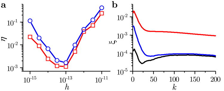
The choice of the time step h for discretizing the dynamics was determined based on its impact on the state estimation error, as shown in Fig. 2. In general, the network cannot be fully observed when the discretization time step is much larger than the dominant time constant in the system. We found that for the combustion networks analyzed here, the optimal choice is h = 10−13 (seconds). Since observing real combustion experiments at the resolution of picoseconds may be possible using femtosecond spectroscopy [51, 52], essentially all but the fastest reacting components could be estimated in a real experiment.
Figure 2.
Accuracy of the discretization methods. (a) Estimation error η as a function of the discretization step size h, for the H2/O2 (squares) and GRI-Mech 3.0 (circles) networks, using the IRK model. (b) Comparison of the time-dependent error for each step k, where is computed using the BE (red line), TI (blue line), and IRK (black line) discretization methods. This comparison is for the H2/O2 network, with N = 200, h = 10−13, and computed using ode15s. In both panels, the results are averaged over 100 realizations of random initial conditions, as defined in equation (23).
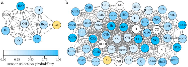
The OIDs are shown in Figs. 3a and b for the H2/O2 and GRI-Mech 3.0 networks, respectively. In each case, the OID consists of two SCCs, of which one has a single node. This node is argon (Ar), which is an inert gas whose concentration remains constant and can influence the concentration of other species through pressure. The large SCC has no incoming edges and is thus a root component in both networks. From the theory proposed in [10], the complete network observability can be ensured by placing a single sensor in the root SCC. Accordingly, in our numerical simulations we make sure that at least one sensor is placed in the large SCC. In addition, before solving the optimization problem (22), we place a sensor on the node forming the small SCC. This way, we avoid scenarios in which the observability measure would numerically overflow due to a badly conditioned Jacobian in (22) (especially when the number of sensor nodes is constrained to be small). More generally, some sensors may be placed a priori in non-root SCCs of any given network (irrespective of the number of SCCs) to avoid similar scenarios. In the context of our approach, these sensor additions can only further improve observability.
Figure 3.
OIDs and sensor selection probabilities for combustion networks. OIDs of the (a) H2/O2 network and (b) GRI-Mech 3.0 network, where self-loops are omitted for clarity. Color-coded is the probability of selecting the node using the optimal sensor selection method (see text). Each network consists of two SCCs, one formed by Ar (always taken as a sensor) and the other by the remaining nodes. The data were computed using the IRK model for N = 200 and h = 10−13.
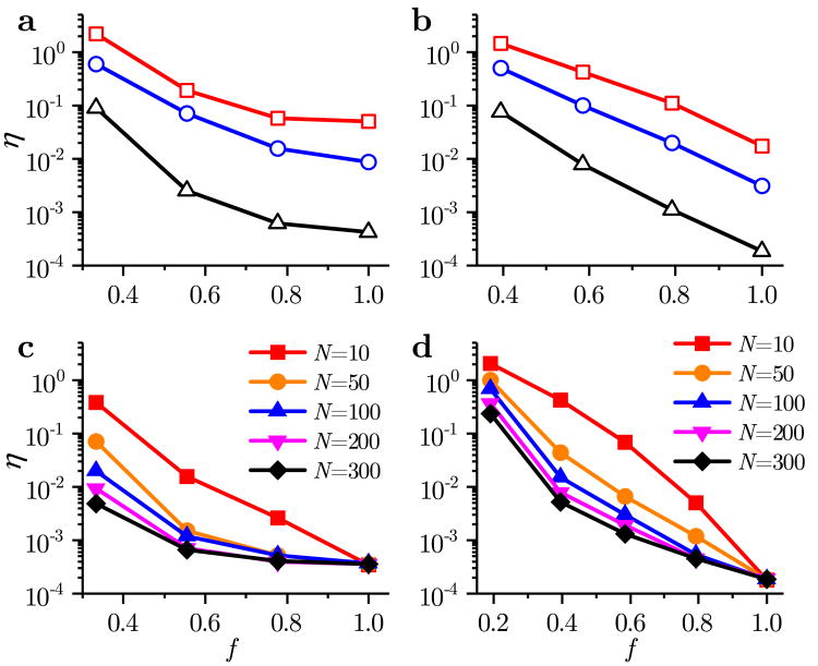
To proceed, we define the sensor fraction f = r/n as the fraction of nodes in the network that are selected as sensors. We first compare the estimation errors η for the three postulated models. The results are shown in Figs. 4a and b for a random sensor selection in the large SCCs. These results show that the IRK model produces the lowest estimation error η, which is consistent with it being more accurate than the BE and TI models. In addition, the IRK model also provides the smallest time-dependent error ξk at every step k, as shown in Fig. 2b. The price of this is the increased computational complexity of the estimation procedure based on the IRK model. Note that all three models exhibit a non-zero estimation error for the sensor fraction f = 1 (i.e., when all nodes are directly observed), which originates from model uncertainties, given that the postulated models only approximate the system used to generate the “real” data.
Figure 4.
Estimation error η as function of the sensor fraction f and observation length N. Results for the (a, c) H2/O2 network and (b, d) GRI-Mech 3.0 network. Panels a and b compare the three models (Δ-IRK, ○-TI, and □-BE) for N = 50, whereas panels c and d compare different N for the IRK model. Each data point is an average over 100 realizations of the random sensor placement and initial guesses of the solution in the GRI-Mech 3.0 network and over all possible placement configurations in the H2/O2 network. The discretization step was h = 10−13 in all simulations.
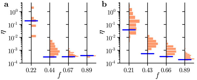
Next, we solve the optimal sensor placement problem given by equation (22) for N = 200 and several values of f, and compute estimation error for the resulting optimal sensor selection. From the results shown in Figs. 5a and b we conclude that the optimal sensor selection method performs significantly better than random sensor selection. Note that the observation horizon length N has a strong influence on the sensor selection performance, which we show in detail in Section V-C.
Figure 5.
Optimal sensor selection for the combustion networks. Estimation error η for the (a) H2/O2 network and (b) GRI-Mech 3.0 network. For each network and sensor fraction f, the histogram presents η for an exhaustive calculation in panel a and for 100 realizations of the random sensor placement in panel b. The blue line marks the estimation error for the calculated optimal sensor selection. The results are generated using the IRK model for N = 200 and h = 10−13.
The probability of selecting the nodes using the optimal sensor selection method is obtained by calculating the frequency with which each node is chosen as a sensor in the solution of the optimal sensor selection problem for the various sensor fractions f used in Fig. 5. In this calculation, the contribution to the selection probabilities is weighted uniformly across different f, since the optimal sensor selection is generally unique for a given f. The probabilities are shown color-coded in Fig. 3.
V-B Applications to biological networks
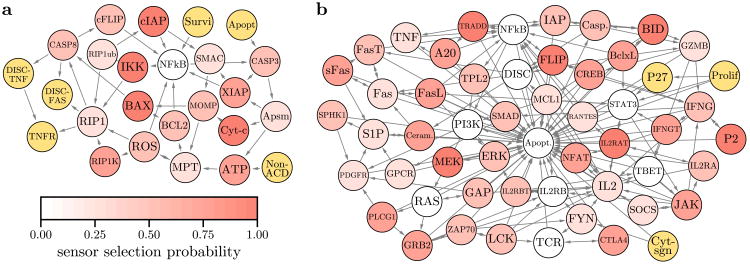
We consider a cell death (CD) regulatory network model [29] and a survival signaling (SS) network model of T cells [28,30], having n = 25 and n = 54 nodes, respectively. Each node in these networks represents a gene, a gene product, or a concept (e.g., apoptosis), which can be active or inactive. Both systems are modeled as Boolean networks, where the activation of one node influences the activation of others. Following the standard practice, we transformed the Boolean relations into continuous-time dynamics using the ODEFY software toolbox [53]; specifically, we used the Hillcube method with the threshold parameter of 0.5. We also simplified the state-space model of the CD and SS networks, as follows. The original CD network contains 28 nodes, however 3 of them are input nodes (FASL, TNF, and FADD), whose values are set to 0.5 in our simulations. This way, they are eliminated from the network. Similarly, the original SS network contains 60 nodes, however 6 of them are input nodes. The input nodes TAX, Stimuli2, and CD45 are set to zero, whereas the other input nodes, Stimuli, IL15, and PDGF, are set to 1. After this simplification, the CD network has 7 SCCs and the SS network has 4 SCCs in the OID, as shown in Fig. 6.
Figure 6.
OIDs and sensor selection probabilities for biological networks. Same as in Fig. 3 for the (a) CD network and (b) SS network. Yellow indicates single-node SCCs, whereas the remaining nodes belong to a giant SCC. Sensors are placed on the yellow nodes a priori, which are then excluded from the optimal sensor selection. The data were computed using the IRK model for N = 100 and h = 0.02 in panel a, and for N = 100 and h = 0.05 in panel b.
The entries of the initial state and the guesses for solving equation (10) are generated from the uniform distribution on the interval (0, 1), where x̄0 and x̄0 are taken to be the vectors of ones and zeros, respectively.
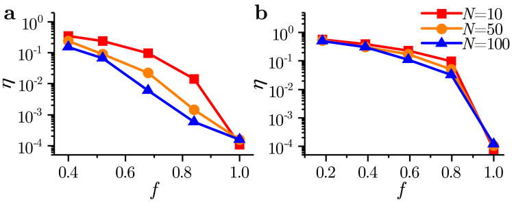
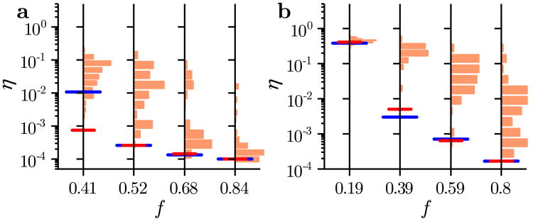
The estimation error, shown in Fig. 7, behaves similarly to the error observed in the combustion networks. The results of the optimal sensor selection are shown in Figs. 8a and b (blue lines), where we compare it with two other approaches. As in Fig. 5b, one approach is essentially graph-theoretic and consists of random placement under the constraint of having at least one sensor in each SCC (histograms). The other approach is a variant of our optimal sensor selection method in which we lift the constraint of having at least one sensor in each SCC (red lines). The results show the significant advantage of our approach compared to the others. The probability of selecting the nodes using the optimal sensor selection method is color-coded in Fig. 6.
Figure 7.
Estimation error η for the (a) CD network and (b) SS network as a function of the observation horizon and sensor fraction. The results are generated for the IRK model with h = 0.02 in panel a and h = 0.05 in panel b. The results are averages over 100 realizations of the random sensor selections and random initial conditions.
Figure 8.
Optimal sensor selection for the biological networks. Estimation error η for the (a) CD network and (b) SS network. For each network and sensor fraction f, the histogram presents η for 100 realizations of the random sensor placement. The blue line marks the estimation error for the calculated optimal sensor selection; the red line indicates the corresponding result when information about the OID is ignored. The results are generated using the IRK model for N = 100 and h = 0.02 in panel a, and for N = 100 and h = 0.05 in panel b.
V-C Comparison to other sensor selection methods
We now compare our sensor selection method to other methods available in the literature. Two main approaches are available, one based on empirical Gramians (which can have various definitions) and the other based on heuristic measures of observability. Further details on these approaches are provided in Appendix C. For our analysis, we specify the following methods:
Method 1. The empirical observability Gramian is computed using Definition 2 (see Appendix B) and the optimal sensor selection is performed by solving the optimization problem in equations (53) and (54).
Method 2. The empirical observability Gramian is computed using Definition 3 (see Appendix B) and the optimal sensor selection is performed by solving the optimization problem in equations (53) and (54).
Method 3. This is our approach.
Method 4. Modified version of our approach, where we use a greedy algorithm [13] instead of the NOMAD method to solve (22).
The motivation behind Method 4 is our conjecture that the cost function in (22) is submodular. If the conjecture is correct then the optimization can be solved by a greedy algorithm efficiently and potentially faster than by the NOMAD solver. However, we leave the proof of this conjecture for future work.
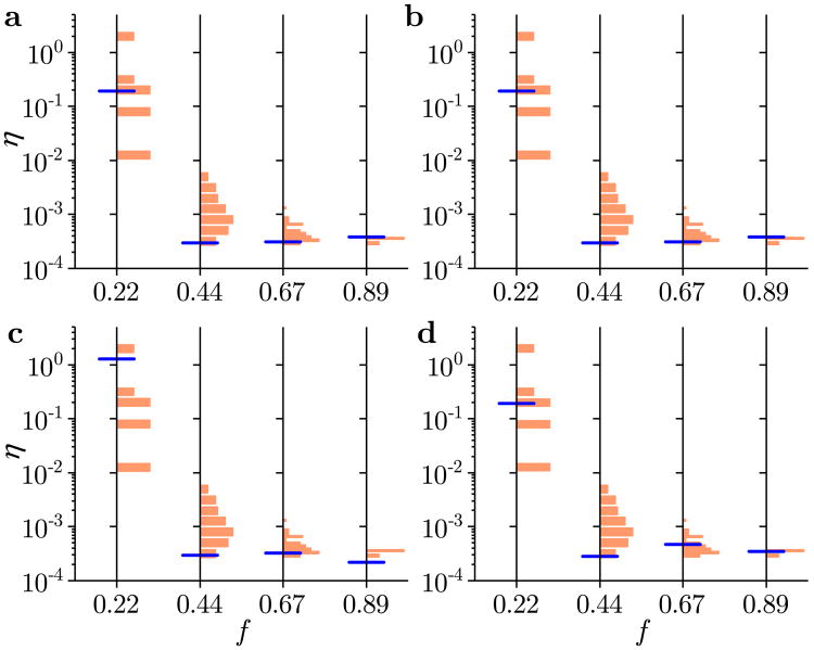
Once the optimal sensor locations are determined, we estimate the initial state and compute the estimation error η. In order to validate the optimal sensor selection procedure, we compare it with a random sensor selection. Namely, in the case of the H2/O2 network, we generate all possible selections of the sensors for certain sensor fractions, whereas in the case of the GRI-Mech 3.0 network we generate 100 random sensor selections, and for such selections we compute the initial state estimates and the estimation errors. In the validation step, the observation data are generated by simulating the network starting from the same initial state that has been used in sensor selection methods to compute the empirical observability Gramians or the cost function in equation (57). This is a “true” state, which is generated using equation (23). The initial guess of the true state is also generated using equation (23), and is generally not equal to the true state. We use h = 10−13, the IRK model, and vary the observation length N to investigate the effect of the observation length on the optimal sensor selection performance.
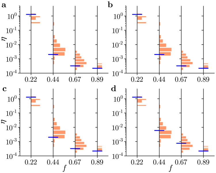
Figure 9 shows the comparison for the H2/O2 network and N = 50. It can be observed that all 4 methods perform relatively poorly compared to the random sensor selection. This is due to the fact that the total number of samples N used in the computation of the cost functions and for the state estimation, is relatively short compared to the slowest time constant in the system. Consequently, the empirical observability Gramians and the Jacobians do not accurately capture the network dynamical behavior. Figure 10 shows the results for the H2/O2 network and N = 200. In sharp contrast to the case of N = 50, shown in Fig. 9, the results shown in Fig. 10 are dramatically improved. We see that the methods perform well compared to a random sensor selection and that their performance is similar. The results can be additionally improved by selecting even larger N, however, at the expense of the increased computational complexity. To quantify the relative performance of the sensor selection methods, we calculate the logarithmic error differences logη(method i) – logη(method 3), for methods i = 1, 2, and 4, respectively. These differences are 0.0, 0.0, and −0.02 for f=0.44. The corresponding differences are −0.01, −0.01, and 0.16 for f=0.67. Finally, the differences are 0.24, 0.24, and 0.21 for f=0.89. It can be observed that, compared to the other Methods, Method 3 (our approach) has similar performance for f=0.44 and f=0.67, while it has a significantly better performance for f=0.89.
Figure 9.
Four methods for sensor selection validated and compared on the H2/O2 network for short observation length. Estimation error η for (a) Method 1, (b) Method 2, (c) Method 3, and (d) Method 4. The histograms correspond to the estimation errors for all possible combinations of the sensor nodes. The network is sufficiently small that exhaustive calculation of all combinations is possible in this case. The blue line represents the estimation error for the optimal sensor selection. The results are obtained for N = 50, h = 10−13, and the IRK model.
Figure 10.
Same as in Fig. 9 for the longer observation time of N = 200.
Comparison of computational complexity
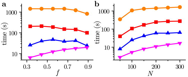
Compared to Methods 1 and 2, which are based on the observability empirical Gramians, the computational complexity of Methods 3 and 4 is much lower. This is because the computation of the empirical observability Gramians requires the network dynamics simulations for a number of perturbations of the initial condition, and each of these simulations have computational time scaling with at least 0(n3). In practice, this computational complexity might be even higher due to model stiffness. On the other hand, to compute the cost functions for Methods 3 and 4, it is only necessary to simulate the dynamics for a single initial condition. This is reflected in the computational times of these methods shown in Fig. 11. Method 3 (our approach) is almost an order of magnitude faster than Method 1, and two orders of magnitude faster than Method 2, across a wide range of parameters. We note that this difference will become even larger for larger networks. Method 4 (variant of our approach) is faster than Method 3 for the parameters shown in Fig. 11, since the greedy algorithm evaluates the objective function fewer times than the NOMAD solver. However, this may not always be the case when both the network size n and the fraction of observed nodes f are large. In such cases, Method 4 may become slower because the number of objective function evaluations is proportional to n × f in this method. On the other hand, the number of objective function evaluations in Method 3 is determined by the convergence thresholds of the solver, which do not necessarily depend on n or f.
Figure 11.
Computational time for sensor selection as a function of (a) the fraction of observed nodes f and (b) the observation horizon N. The various curves correspond to Method 1 (■), Method 2 (●), Method 3 (▴), and Method 4 (▾), applied to the GRI-Mech 3.0 network. Results are averaged over 10 random initial guesses for the selected sensors, using the IRK model and h = 10−13, for N = 200 in panel a and f = 0.5 in panel b.
V-D Discussion of the results
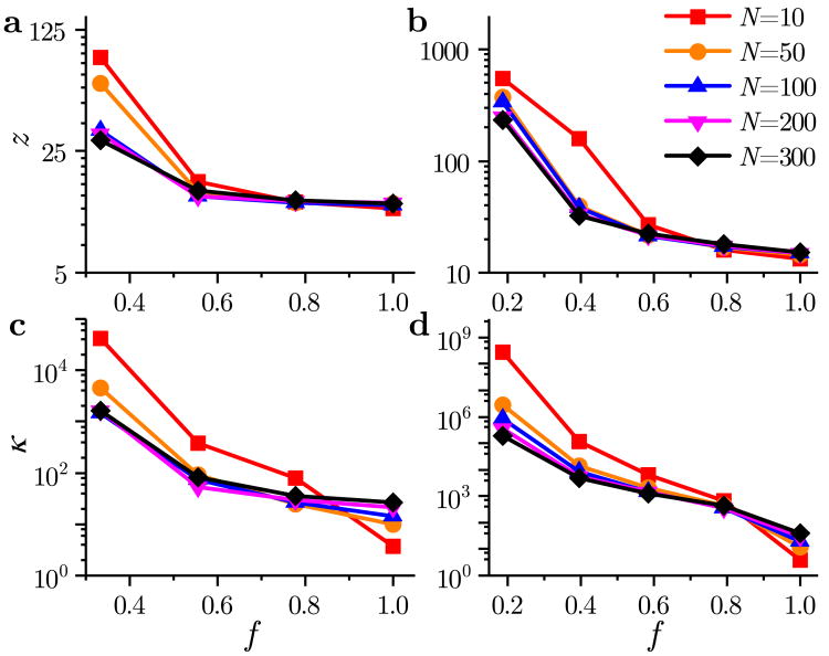
Figures 4c and d indicate a trade-off between the sensor fraction f and the observation length N against the estimation error η. The results show that there exists a fundamental obstacle in decreasing η below a certain value for small f. Additional error reduction can be achieved by significantly increasing the observation length N, but our results show that η starts to saturate for larger values of N. Furthermore, the value of N is usually constrained by the available computational power and the necessarily limited number of measurements in real experiments, and it cannot be increased to infinity. On the other hand, for small f, the estimation procedure becomes ill-conditioned and the number of iterations of the TRR method dramatically increases (see Fig. 12). This implies that, in practice, the observation performance can be severely degraded by measurement noise and that we need more time to compute the estimate when the fraction of observed nodes is smaller.
Figure 12.
Convergence and condition numbers of Jacobians of the nonlinear least-squares problem defined by equation (10). (a, b) Number of iterations z to compute the estimate as a function of the sensor fraction f and the observation horizon N. (c, d) Condition number κ of the Jacobian matrix at the final estimate. Panels a and c correspond to the H2/O2 network, panels b and d correspond to the GRI-Mech 3.0 network. The parameters are the same as the ones used in Fig. 4, panels c and d.
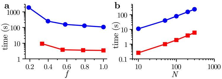
For the networks we consider, our sensor selection procedure ensures that at least one sensor node is selected within each SCC of the OID. From a purely structural analysis of Figs. 3 and 6, it would appear that the initial state could be reconstructed from the measurements of these sensors. However, from our results, it follows that in practice this is not possible in general. As the sensor fraction f approaches a small number, the estimation error η dramatically increases. Furthermore, the number of iterations of the TRR method also dramatically increases, implying that the time to compute the estimate significantly increases (see Fig. 13a). We have verified through supplementary simulations that these conclusions are still valid even if the data-generating model is the same as the model postulated for observing the state. This suggests that the observed behavior does not originate from the model uncertainties alone—it can also be caused by limitations in numerical precision. In the extreme case of a large network with a fraction of sensor nodes that is too small, we would need an enormous amount of time to compute the estimate, and the estimation error would be large. In the case of small sensor fractions, the estimation error η can be decreased by increasing N; however, larger N also increases the computational complexity of the estimation method, as illustrated in Fig. 13b.
Figure 13.
Computational complexity of solving the nonlinear least-squares problem defined by equation (10). The computational complexity is shown for the H2/O2 (■) and GRI-Mech 3.0 (●) networks as a function of (a) the fraction of the observed nodes f and of (b) the observation horizon N. In panel a the results correspond to an average of 100 samples of randomly selected sensors and N = 200, whereas in panel b the results correspond to f = 0.6. In both panels, the results are obtained for the IRK model and h = 10−13.
For completeness, we have tested potential correlations with several node centrality metrics: betweenness centrality, closeness centrality, degree (both in- and out-degrees), and pagerank, which were calculated for every network studied here. In some cases we observe that the nodes selected by the optimal sensor selection method have larger than average centrality values, but beyond that we observe no clear correlation between individual centrality measures and the probability of selecting a node. The correlation coefficients between sensor selection probability and centrality measures are summarized in Appendix D. For the H2/O2 network, the most probable sensor nodes are the primary reactants and products, namely, H2, O2, and H2O. For the GRI-Mech 3.0 network, this is only partially true; several probable sensor nodes are main reactants and products, such as CH4, O2, and H2O, but others are unstable radicals, such as CH3 and C2H5. We can only conclude that these species are selected because they carry the most information about the dynamics of other species in the mechanism. Similar conclusions hold for the biological networks as well. For example, in the CD network, two of the most frequently selected nodes (BAX and IKK) are primers for certain activation pathways [29].
VI Conclusions
Our results indicate that there is a fundamental limitation in network state estimation that, to the best of our knowledge, has not been considered before. This limitation stems from the complex interaction between three quantities: the number of available sensors, the observation length, and the condition number of the system's Jacobian. While in principle the estimation accuracy can be improved by increasing the number of sensors and the observation length, this is usually not feasible in practice. Apart from physical limitations of a real system (i.e., the number of available sensors, and the amount of available data), the fundamental limitation is the amount of computation needed to calculate the state estimate. Either the improvement of the condition number requires an unrealistic amount of data to be processed, or the number of iterations (and precision) remains too large due to bad conditioning. The best possible balance between these limitations for a given system can be found by our approach to optimal sensor selection. The results on the latter clearly illustrate the great potential of our framework compared to what would be possible with purely graph-theoretic approaches or approaches based on empirical Gramians, particularly as the number of SCCs and state variables increase. Our optimal sensor selection method indeed proves to be extremely useful in scenarios involving combinatorial explosion, such as in the case of large networks.
Acknowledgments
This research was supported in part by MURI Grant No. ARO-W911NF-14-1-0359, in part by Simons Foundation Award No. 342906, and in part by NCI CR-PSOC Grant No. 1U54CA193419.
Appendices.
A Combustion networks
A combustion network is defined by
| (24) |
where Mi, i = 1, 2, …, n, are chemical species (e.g., H, O, or H2), n and nr are the total numbers of chemical species and reactions, respectively, and αji and βji are stoichiometric coefficients. To equation (24) we assign n coupled differential equations of the form [34]
| (25) |
where xi ∈ ℝ≥0 is the concentration of the species Mi, x = col (x1, x2, …, xn) ∈ ℝn is the vector of concentrations (state vector), and qj is a polynomial function. This function has the following form:
| (26) |
where are the forward and backward reaction rates. The equations in (25) can be written compactly as
| (27) |
where qc (x) = col (q1 (x), q2 (x), …, qnr (x)) and the matrix Γ = [γij] ∈ ℝn×nr has entries γij = βji – αji. Equation (27) is the state-space model of the combustion networks.
B Empirical Gramians of Nonlinear Systems
Some of the approaches proposed in the literature for sensor placement are based on the concept of empirical observability Gramian of nonlinear systems [14–18]. Here, we review previous definitions of the empirical observability Gramian and introduce a new definition that is more suitable for the class of network systems we consider. We also provide guidelines for numerical computation and parameter selection.
Definition 1
We first consider the definition of the empirical observability Gramian introduced in [15]. Let 𝒯n = {T1, T2, …, Tυ} be a set of υ orthogonal, n×n matrices; ℳ = {c1, c2, …, cs} be a set of s positive constants; and let ℰn = {e1, e2, …, en} be a set of n standard unit vectors in ℝn. Furthermore, let us introduce the mean ū of an arbitrary vector u as follows:
| (28) |
For the network dynamics with an output equation,
| (29) |
| (30) |
the empirical observability Gramian X̂1 ∈ ℝn×n is defined by
| (31) |
Here Ψlm(t) ∈ ℝn×n is a matrix whose (i, j)th entry is defined by
| (32) |
where yilm(t) is the output of the network corresponding to the initial condition x0 = cmTlei. The sets ℳ and 𝒯n are chosen by the user. Typical choices reported in the literature are [14, 15]: ℳ = {0.25, 0.5, 0.75, 1} and 𝒯n = {In, −In}.
Definition 2
An alternative definition of the empirical observability Gramian [16, 17] is
| (33) |
where
| (34) |
Here the vector y±i (t), i = 1, 2, …, n, is the output of the network at the time t for the initial condition x0 ± γei, where x0 is an arbitrary vector and γ > 0 is a user choice. This definition is more attractive from the computational point of view, compared to the definition in equation (31), because with the choice of the initial condition x0 we can freely choose the initial point around which we want to compute the empirical Gramian.
Definition 3
The initial conditions x0 ± γei used to compute the empirical observability Gramian in equation (33), are not the most optimal choices from the computational point of view. Namely, γei perturbs x0 only in a single direction. We would like to construct a perturbation that is richer, such as the perturbation cmTlei used to compute the empirical observability Gramian in equation (31) (where Tl is not an identity matrix). This motivates us to combine the above two definitions into a single one definition. We define the empirical observability Gramian as the following matrix:
| (35) |
where
| (36) |
and y±ilm(t), i = 1, 2, …, n, is the output of the network at time t for the initial condition x0 ± cmTlei, where x0 is an arbitrary vector.
It can be easily shown that in the case of the linear dynamics
| (37) |
| (38) |
where A ∈ ℝn×n and C ∈ ℝr×n are the constant system matrices, and for τ = ∞in (33), the definitions in equations (31) and (33) become equal to the observability Gramian of the linear system given in equations (37) and (38):
| (39) |
where exp(At) ∈ ℝn×n is the matrix exponential. In the sequel we show that the definition in equation (35) is equal to the definition given in equation (39) for linear systems. For the linear dynamics in equations (37) and (38), and an arbitrary initial condition z ∈ ℝn, we have
| (40) |
From equation (40), it follows that
| (41) |
which implies that the (i, j)th entry of the matrix Φlm(t)TΦlm(t) in equation (35) is given by
| (42) |
On the other hand,
| (43) |
where Z = [zi,j] is an arbitrary matrix. From equations (42) and (43), we have
| (44) |
The last expression implies that
| (45) |
which for τ = ∞ in equation (35) reduces to equation (39).
Computation of the observability Gramians
To compute any of the empirical observability Gramians previously introduced, we first need to approximate the integrals. We use a trapezoidal method for approximating integrals because its computational complexity is low. To compute the expressions in equation (35), we need to approximate the integral
| (46) |
where
| (47) |
First we divide [0, τ] into Q segments divided by points
| (48) |
The approximation of χ is defined by
| (49) |
where Δti = ti – ti–1. Taking this into account, the approximate empirical Gramian of X̄3, has the following form:
| (50) |
Similarly, we can define the approximate Gramians of X̂1 and X̂2.
To compute equation (50), we need to evaluate the matrix function Flm(ti) at the discrete-time steps ti, i = 0, 1, …, Q. This requires the knowledge of the state sequences x(ti) from different initial states. For simplicity, we choose equidistant time steps Δti = const. In the results reported in Section V-C, the discrete-time sequences are computed on the basis of the IRK model.
Parameter choice of the observability Gramians
To compute the empirical observability Gramians we need to choose the sets 𝒯n and ℳ, the parameters γ and τ, as well as the initial condition x0. The principle for choosing these parameters is that all the initial states from which the computation of the state trajectory starts, should be within the physical limits of the state variables. For example, in the case of the combustion networks, the entries of the initial states should be positive, whereas in the case of the biological networks the entries of the initials states should be in the interval [0, 1]. For brevity, we explain the parameter selection for the case of combustion networks. Similar principles can be used in the case of biological networks. In all three definitions, the initial conditions are specified by equation (23).
In Definition 1, we choose 𝒯n = {In} (unlike the choice of {In, −In} reported in [14, 15]) and ℳ = {0.25, 0.5, 0.75, 1}. The improper integral is approximated by replacing the ∞ by a finite value τ. A rule of thumb for the selection of the parameter τ is to choose it in such a way that for an arbitrary initial condition the majority of state trajectories approximately reach the steady states. However, because the computational complexity of computing the empirical observability Gramians increases with τ, its value should not be very large. That is, there is a trade-off between the computational complexity and the value of τ. As we show in Section V-C, the value of τ dramatically influences the results, and it should be as large as possible.
In Definition 2, we choose γ = 0.5. Our numerical results show that for the selection of the initial condition given by equation (23), the entries of the perturbed initial conditions (almost) always stay positive. The value of τ is selected in the same manner as in Definition 1.
In Definition 3, the matrices Ti that are elements of the set 𝒯n are chosen using the following procedure. First, we generate random matrices Si, i = 1, 2, …, υ, whose entries are drawn from the standard normal distribution. After these matrices are constructed, we perform QR decompositions [6]:
| (51) |
The matrix Qi is orthogonal, and consequently, we chose Ti = Qi for all i. With this choice of Ti we are able to perturb more directions in the state-space around x0 compared to selecting Ti as identity matrices. The set ℳ is chosen as ℳ = {0.25, 0.5, 0.75, 1}. Our results show that for such a selection of Tn and ℳ, and for the selection of the initial condition given by equation (23), the perturbed initial states almost always stay positive. The value of τ is selected in the same manner as in Definition 1.
C Existing approaches for optimal sensor selection
We briefly summarize the two approaches from the literature against which our optimal sensor selection method is compared in Section V-C.
The starting point of both approaches is the parameterized output equation:
| (52) |
where C1(b) = diag (b) ∈ ℝn×n and b ∈ ℝn is the parametrization vector. Once we have selected the sensors, the matrix C1 is compressed into the matrix C ∈ ℝr×n that is used to define the output equation (2).
First approach
The first approach is based on the empirical observability Gramians defined in Appendix B. This approach is explained on the example of the empirical observability Gramian introduced in Definition 3. It can be easily modified such that it is based on the empirical Gramians introduced in the other two definitions.
We start from the approximate empirical Gramian X̄3 defined in equation (50). By substituting equation (52) into equation (36), the matrix Φlm(t) becomes a function of the parametrization vector b, that is, Φlm(t) = Φlm(t, b). Then, substituting such an expression in equation (47), we similarly obtain that Flm = Flm(t, b). This implies that the approximate Gramian in equation (50) also becomes a function of the parametrization vector b: X̄3 = X̄3 (b).
Several criteria have been used to quantify the degree of observability using empirical Gramians. Widely used criteria are the minimal singular (eigenvalue), trace, condition number, and the determinant of the empirical observability Gramian [14, 16, 18]. The degree of observability based on the matrix determinant is attractive from the optimization point of view, mainly because the matrix determinant is a smooth function of the matrix entries [14]. Accordingly, we measure the degree of observability using the matrix determinant. Similarly to equation (22), the optimal sensor locations are determined as the solution of the following optimization problem:
| (53) |
| (54) |
We solve this optimization problem using the NOMAD solver implemented in the OPTI toolbox [14, 48, 49].
Second approach
An elegant approach to the sensor selection for linear systems has been developed in [13]. This approach determines the optimal sensor locations by performing a finite number of evaluations of a set function that measures the observability degree of a network. It is shown that this method works well for linear systems provided that the set function is submodular (for more details, see [13]). Although it is developed for linear systems, we apply this approach to nonlinear systems without providing explicit proofs that justify the application of such a method for nonlinear systems. Our results show that this approach works relatively well even for nonlinear systems.
Let V = {1, 2, …, n} be a set where n is the total number of nodes in our network. Let a set function l : 2V → ℝ assign a real number to each subset S of V. The subset S is the set of sensors that we want to choose. For example, if we select S = {1, 2, 9} then for such a choice, the function l returns a real value quantifying the degree of observability. The problem of optimal sensor selection of r nodes can be formulated as the following optimization problem:
| (55) |
It is easy to see that the optimization problems defined in equations (53) and (54), and in equations (22), belong to the same class of optimization problems as the optimization problem in equation (55). The greedy algorithm for solving the optimization problem in equation (55) has the following form. We start with an empty set S0, then for i = 1, 2, … r and perform the following two steps:
Compute the gain Δ (a|Si) = l (Si ∪ {a}) – l (Si) for all elements a ∈ V \ Si.
Define the set Si+1 by adding the element a to the set Si with the highest gain,
| (56) |
It is known that the greedy algorithm performs well for submodular functions l. In [13], it is shown that the logdet(·) function of the controllability Gramian of a linear system is submodular. Motivated by this we define the function l to be
| (57) |
where x0 is fixed and it is not considered as an argument of the l function and J1 (b, x0) is the Jacobian used in equation (20). In equation (57) we slightly abuse the notation since l is originally defined as a function that maps the set S into a real value. On the other hand, the definition in equation (57) maps an n-dimensional vector into a real value. However, the sensors are marked by the position of the non-zero entries of b. The proof of the submodularity of the function l defined in equation (57) is left out and it is a future research topic.
D Sensor selection and centrality measures
The correlations between sensor placement and centrality measures are reported in Table 2.
Table 2.
Correlation coefficients between the probability of selecting a node as a sensor (shown color-coded in Figs. 3 and 6) and various node's centrality measures in the OID.
| Centrality | H2/O2 | GRI-Mech 3.0 | CD | SS |
|---|---|---|---|---|
| in-degree | −0.57 | −0.02 | −0.63 | −0.37 |
| out-degree | −0.55 | −0.04 | −0.50 | 0.06 |
| in-closeness | −0.57 | −0.05 | −0.52 | −0.40 |
| out-closeness | −0.55 | −0.19 | −0.43 | 0.05 |
| betweenness | −0.09 | −0.13 | −0.69 | −0.38 |
| pagerank | −0.57 | −0.02 | −0.03 | −0.25 |
Contributor Information
Aleksandar Haber, Department of Physics and Astronomy, Northwestern University, Evanston, IL 60208 USA, when this research was performed. He is now with the Department of Engineering Science and Physics, City University of New York, College of Staten Island, Staten Island, NY 10314 USA.
Ferenc Molnar, Department of Physics and Astronomy, Northwestern University, Evanston, IL 60208 USA.
Adilson E. Motter, Department of Physics and Astronomy, Northwestern University, Evanston, IL 60208 USA
References
- 1.Camacho EF, Alba CB. Model Predictive Control. London: Sprinver-Verlag; 2007. [Google Scholar]
- 2.Khalil HK. Nonlinear Systems. Upper Saddle River, NJ: Prentice Hall; 2002. [Google Scholar]
- 3.Whalen AJ, Brennan SN, Sauer TD, Schiff SJ. Observability and controllability of nonlinear networks: the role of symmetry. Phys Rev X. 2015;5:011005. doi: 10.1103/PhysRevX.5.011005. [DOI] [PMC free article] [PubMed] [Google Scholar]
- 4.Yan G, et al. Spectrum of controlling and observing complex networks. Nat Phys. 2015;11:779–786. [Google Scholar]
- 5.Lin F, Fardad M, Jovanović MR. Design of optimal sparse feedback gains via the alternating direction method of multipliers. IEEE Trans Autom Control. 2013;58:2426–2431. [Google Scholar]
- 6.Verhaegen M, Verdult V. Filtering and System Identification: A Least Squares Approach. New York, NY: Cambridge University Press; 2007. [Google Scholar]
- 7.Timme M. Revealing network connectivity from response dynamics. Phys Rev Lett. 2007;98:224101. doi: 10.1103/PhysRevLett.98.224101. [DOI] [PubMed] [Google Scholar]
- 8.Haber A, Verhaegen M. Subspace identification of large-scale interconnected systems. IEEE Trans Autom Control. 2014;59:2754–2759. [Google Scholar]
- 9.Isidori A. Nonlinear Control Systems. London: Springer Science & Business Media; 2013. [Google Scholar]
- 10.Liu YY, Slotine JJ, Barab´si AL. Observability of complex systems. Proc Natl Acad Sci. 2013;110:2460–2465. doi: 10.1073/pnas.1215508110. [DOI] [PMC free article] [PubMed] [Google Scholar]
- 11.Fiedler B, Mochizuki A, Kurosawa G, Saito D. Dynamics and control at feedback vertex sets. I: Informative and determining nodes in regulatory networks. J Dyn and Diff Eq. 2013;25:563–604. doi: 10.1016/j.jtbi.2013.06.009. [DOI] [PubMed] [Google Scholar]
- 12.Mochizuki A, Fiedler B, Kurosawa G, Saito D. Dynamics and control at feedback vertex sets. II: A faithful monitor to determine the diversity of molecular activities in regulatory networks. J Theo Bio. 2013;335:130–146. doi: 10.1016/j.jtbi.2013.06.009. [DOI] [PubMed] [Google Scholar]
- 13.Summers TH, Cortesi FL, Lygeros J. On submodularity and controllability in complex dynamical networks. IEEE Trans Control Netw Syst. 2016;3:91–101. [Google Scholar]
- 14.Qi J, Sun K, Kang W. Optimal PMU placement for power system dynamic state estimation by using empirical observability Gramian. IEEE Trans Power Syst. 2015;30:2041–2054. [Google Scholar]
- 15.Lall S, Marsden JE, Glavaški S. A subspace approach to balanced truncation for model reduction of nonlinear control systems. Int J Robust Nonlin. 2002;12:519–535. [Google Scholar]
- 16.Krener AJ, Ide K. Measures of unobservability. Proc 48th IEEE Conf on Decision and Control. 2009:6401–6406. [Google Scholar]
- 17.Powel ND, Morgansen KA. Empirical observability Gramian rank condition for weak observability of nonlinear systems with control. Proc 54th IEEE Conf on Decision and Control. 2015:6342–6348. [Google Scholar]
- 18.Singh AK, Hahn J. Determining optimal sensor locations for state and parameter estimation for stable nonlinear systems. Ind Eng Chem Res. 2005;44:5645–5659. [Google Scholar]
- 19.Simon D. Optimal State Estimation: Kalman, H Infinity, and Nonlinear Approaches. Wiley; 2006. [Google Scholar]
- 20.Julier SJ, Uhlmann JK. New extension of the Kalman filter to nonlinear systems. Proc SPIE. 1997;3068:182–193. [Google Scholar]
- 21.Stano PM, Lendek Zs, Babuška R. Saturated Particle Filter: Almost sure convergence and improved resampling. Automatica. 2013;49:147–159. [Google Scholar]
- 22.Stano PM, Lendek Zs, Braaksma J, Babuška R, de Keizer C, den Dekker AJ. Parametric Bayesian Filters for Nonlinear Stochastic Dynamical Systems: A Survey. IEEE T Cybernetics. 2013;43:1607–1627. doi: 10.1109/TSMCC.2012.2230254. [DOI] [PubMed] [Google Scholar]
- 23.Morall P, Grizzle J. Observer design for nonlinear systems with discrete-time measurements. IEEE Trans Autom Control. 1995;40:395–404. [Google Scholar]
- 24.Alessandri A, Baglietto M, Battistelli G. Moving-horizon state estimation for nonlinear discrete-time systems: New stability results and approximation schemes. Automatica. 2008;44:1753–1765. [Google Scholar]
- 25.Abarbanel HDI, Creveling DR, Farsian R, Kostuk M. Dynamical State and Parameter Estimation. SIAM J Appl Dyn Syst. 2009;8:1341–1381. [Google Scholar]
- 26.Rawlings JB, Bakshi BR. Particle filtering and moving horizon estimation. Comput Chem Engin. 2006;30:1529–1541. [Google Scholar]
- 27.Patwardhan SC, Narasimhan S, Jagadeesan P, Gopaluni B, Shah SL. Nonlinear bayesian state estimation: A review of recent developments. Control Engin Practice. 2012;20:933–953. [Google Scholar]
- 28.Saadatpour A, Wang RS, Liao A, Liu X, Loughran TP, Albert I, Albert R. Dynamical and structural analysis of a T cell survival network identifies novel candidate therapeutic targets for large granular lymphocyte leukemia. PLoS Comput Biol. 2011;7:e1002267. doi: 10.1371/journal.pcbi.1002267. [DOI] [PMC free article] [PubMed] [Google Scholar]
- 29.Calzone L, Tournier L, Fourquet S, Thieffry D, Zhivotovsky B, Barillot E, Zinovyev A. Mathematical modelling of cell-fate decision in response to death receptor engagement. PLoS Comput Biol. 2010;6:e1000702. doi: 10.1371/journal.pcbi.1000702. [DOI] [PMC free article] [PubMed] [Google Scholar]
- 30.Zhang R, Shah MV, Yang J, Nyland SB, Liu X, Yun JK, Albert R, Loughran TP., Jr Network model of survival signaling in large granular lymphocyte leukemia. Proc Natl Acad Sci USA. 2008;105:16308–16313. doi: 10.1073/pnas.0806447105. [DOI] [PMC free article] [PubMed] [Google Scholar]
- 31.Turns SR. An Introduction to Combustion: Concepts and Applications. New York, NY: McGraw-Hill; 1996. [Google Scholar]
- 32.Maas U, Pope SB. Simplifying chemical kinetics: intrinsic low-dimensional manifolds in composition space. Combust Flame. 1992;88:239–264. [Google Scholar]
- 33.Smirnov NN, Nikitin VF. Modeling and simulation of hydrogen combustion in engines. Int J Hydrogen Energ. 2014;39:1122–1136. [Google Scholar]
- 34.Perini F, Galligani E, Reitz RD. An analytical Jacobian approach to sparse reaction kinetics for computationally efficient combustion modeling with large reaction mechanisms. Energy Fuels. 2012;26:4804–4822. [Google Scholar]
- 35.Conaire MÓ, Curran HJ, Simmie JM, Pitz WJ, Westbrook CK. A comprehensive modeling study of hydrogen oxidation. Int J Chem Kinet. 2004;36:603–622. [Google Scholar]
- 36.Smith GP, Golden DM, Frenklach M, Moriarty NW, Eiteneer B, Goldenberg M, Bowman CT, Hanson RK, Song S, Gardiner WC, Jr, Lissianski VV, Qin Z. GRI-Mech 3.0. [Accessed: 01/01/2017]; http://www.me.berkeley.edu/grimech/
- 37.Cornelius SP, Kath WL, Motter AE. Realistic control of network dynamics. Nature Comm. 2013;4:1942. doi: 10.1038/ncomms2939. [DOI] [PMC free article] [PubMed] [Google Scholar]
- 38.Zanudo JGT, Albert R. Cell fate reprogramming by control of intracellular network dynamics. PLoS Comput Biol. 2015;11(4):e1004193. doi: 10.1371/journal.pcbi.1004193. [DOI] [PMC free article] [PubMed] [Google Scholar]
- 39.Wells DK, Kath WL, Motter AE. Control of stochastic and induced switching in biophysical networks. Phys Rev X. 2015;5:031036. doi: 10.1103/PhysRevX.5.031036. [DOI] [PMC free article] [PubMed] [Google Scholar]
- 40.Iserles A. A First Course in the Numerical Analysis of Differential Equations. New York, NY: Cambridge University Press; 2009. [Google Scholar]
- 41.Hanba S. On the “uniform” observability of discrete-time nonlinear systems. IEEE Trans Autom Control. 2009;54:1925–1928. [Google Scholar]
- 42.Dennis JE, Jr, Schnabel RB. Numerical Methods for Unconstrained Optimization and Nonlinear Equations. SIAM. 1996 [Google Scholar]
- 43.Byrd RH, Schnabel RB, Shultz GA. Approximate solution of the trust region problem by minimization over two-dimensional subspaces. Math Prog. 1988;40:247–263. [Google Scholar]
- 44.Moré JJ, Sorensen DC. Computing a trust region step. SIAM J Sci Stat Comp. 1983;4:553–572. [Google Scholar]
- 45.Coleman TF, Verma A. A preconditioned conjugate gradient approach to linear equality constrained minimization. Compt Optim Appl. 2001;20:61–72. [Google Scholar]
- 46.Sorensen DC. Minimization of a large-scale quadratic function subject to a spherical constraint. SIAM J Optimiz. 1997;7:141–161. [Google Scholar]
- 47.Ljung L. System identification. Upper Saddle River, NJ: Prentice Hall; 1999. [Google Scholar]
- 48.Le Digabel S. Algorithm 909: NOMAD: Nonlinear optimization with the MADS algorithm. ACM T Math Software. 2011;37:44. [Google Scholar]
- 49.Currie J, Wilson DI. OPTI: Lowering the barrier between open source optimizers and the industrial MATLAB user. Proc Foundations of Computer-Aided Process Operations. 2012:32–37. [Google Scholar]
- 50.Goodwin DG, Moffat HK, Speth RL. Cantera: An object-oriented software toolkit for chemical kinetics, thermodynamics, and transport processes. [Accessed: 08/15/2016]; http://www.cantera.org.
- 51.Couris S, Kotzagianni M, Baskevicius A, Bartulevicius T, Sirutkaitis V. Combustion diagnostics with femtosecond laser radiation. J Phys: Conf Ser. 2014;548:012056. [Google Scholar]
- 52.Li HL, Xu HL, Yang BS, Chen QD, Zhang T, Sun HB. Sensing combustion intermediates by femtosecond filament excitation. Optics Lett. 2014;38:1250–1252. doi: 10.1364/OL.38.001250. [DOI] [PubMed] [Google Scholar]
- 53.Wittmann DM, Krumsiek J, Saez-Rodriguez J, Lauffenburger DA, Klamt S, Theis FJ. Transforming boolean models to continuous models: methodology and application to T-cell receptor signaling. BMC Syst Biol. 2009;3:98. doi: 10.1186/1752-0509-3-98. [DOI] [PMC free article] [PubMed] [Google Scholar]


