Characterization of coronary artery pathological formations from OCT imaging using deep learning

Abstract

Coronary artery disease is the number one health hazard leading to the pathological formations in coronary artery tissues. In severe cases, they can lead to myocardial infarction and sudden death. Optical Coherence Tomography (OCT) is an interferometric imaging modality, which has been recently used in cardiology to characterize coronary artery tissues providing high resolution ranging from 10 to 20 µm. In this study, we investigate different deep learning models for robust tissue characterization to learn the various intracoronary pathological formations caused by Kawasaki disease (KD) from OCT imaging. The experiments are performed on 33 retrospective cases comprising of pullbacks of intracoronary cross-sectional images obtained from different pediatric patients with KD. Our approach evaluates deep features computed from three different pre-trained convolutional networks. Then, a majority voting approach is applied to provide the final classification result. The results demonstrate high values of accuracy, sensitivity, and specificity for each tissue (up to 0.99 ± 0.01). Hence, deep learning models and especially, majority voting method are robust for automatic interpretation of the OCT images.

1. Introduction

Coronary artery disease is the number one health hazard leading to intimal hyperplasia, media disappearance, lamellar calcification, fibrosis, macrophage, and neovascularization, which are the most distinguished pathological formations in coronary artery tissues. In severe cases, they can lead to myocardial infarction and sudden death [1, 2]. In the normal three-layered structure of coronary artery using OCT imaging, intima is characterized as a signal rich well-delineated layer and media appears as a homogeneous signal poor pattern specified by the internal and external elastic lamina. The outermost layer is adventitia, which is characterized as a signal rich layer [1, 3–5]. Intimal hyperplasia is thickening of the intima and can be followed by media destruction since media becomes thinner and finally disappeared as a result of plaque accumulation and vessel remodeling. Intimal thickening can disturb oxygen diffusion and cause proliferation of vasa vasorum in inner layers of the arterial wall, which is called neovascularization. Presence of neovascularization may be a sign of plaque instability and rupture and is characterized in OCT images as signal poor voids [6]. Fibrosis is scarring of the connective tissues, which may occur as a result of the arterial inflammation and is characterized as signal rich areas in OCT imaging. Macrophage may be accumulated within a fibrous cap as a result of monocytes differentiation in confronting with arterial wall inflammation. Macrophage is visualized as a confluent signal rich focal area in OCT imaging [5, 7–10]. Vascular smooth muscle cells (VSMCs) regulate mineralization in intima and media. Rising lipid content within arterial lesions and inflammatory mediators may transform vascular smooth muscle cells into an osteoblast phenotype, resulting in intimal calcification. Calcification may be extended within a fibrous cap, which is visualized as a signal poor area with sharply delineated borders in OCT imaging [5, 11, 12].

Kawasaki Disease (KD), mucocutaneous lymph node syndrome, is an acute childhood vasculitis syndrome, which is the leading cause of coronary artery sequelae, complicated by coronary artery aneurysms with subsequent intimal hyperplasia, media disappearance, neovascularization, fibrosis, calcification, and macrophage accumulation [1, 13]. Progression of pathological formations caused by coronary artery disease can be followed by acute coronary syndrome (ACS). Therefore, it is significant to develop robust coronary artery tissue characterization techniques to evaluate the pathological formations [14].

While conventional imaging techniques such as CT and MRI may be used for clinical assessment of the coronary arteries, they are limited to providing useful information about the underlying coronary artery tissue layers. Also, they are restricted to reflect the histological reality of the regressed aneurysmal coronary segments, which are inappropriately considered as normal coronary segments [1, 3, 4, 13]. Catheter-based Intravascular Ultrasound (IVUS) has been used for many years in interventional cardiology to evaluate coronary artery tissues by providing information on coronary arterial wall and lumen [15]. IVUS imaging is restricted to be used in pediatric cardiology due to its suboptimal spatial imaging resolution (100–150 µm), and low pullback speed. Arterial plaque formations are structural abnormalities, which require an imaging modality with high-resolution to be detected [3, 7].

Cardiovascular Optical Coherence Tomography (OCT) is a catheter-based invasive imaging modality, which typically employs a near-infrared light to provide cross-sectional images of the coronary artery at depth of several millimeters relying on low-coherence interferometry. The unique characteristic of OCT is its high axial resolution of 10–15 µm, which is measured by the light wavelength and is decoupled from the lens dependent lateral resolution ranging from 20–40 µm. The image-wire is inserted into the coronary artery using an over-the-wire balloon catheter from patient’s groin. A sequence of cross-sectional images of coronary artery segment is recorded using the backscattered light from the arterial wall through each pullback. Considering the fact that light can be attenuated by blood before reaching the vessel wall, blood clearance is required before starting the image acquisition [16–18].

1.1. Related works

Automated tissue analysis and plaque detection were focused on 2D intracoronary OCT images in adult patients to visualize plaque formations [19–25]. Combination of light backscattering and attenuation coefficients have been estimated from intracoronary time domain OCT for three different atherosclerosis tissues, namely calcification, lipid pool, and fibrosis [19]. Fibrosis and calcification in coronary atherosclerosis was detected by estimating the optical attenuation coefficient. The estimated values were compared with histopathological features of each tissue to determine the corresponding optical properties [20]. Another study proposed a tissue classification method using Support Vector Machine (SVM) with the combination of texture features and optical attenuation coefficient extracted form atherosclerotic tissues [21]. Another study focused on volumetric estimation of backscattered intensity and attenuation coefficient. [22]. Classification approach using SVM was used to discriminate between fibrosis, calcification, and lipid. Another group were focused on identification and quantification of fibrous tissue based on Short-Time Fourier Transform (STFT) using OCT imaging. [23]. A classification framework is developed to detect normal myocardium, loose collagen, adipose tissue, fibrotic myocardium, and dense collagen. Graph searching method is applied to segment various tissue layers of the coronary artery. Combination of texture features and optical properties of tissues is used to train a relevance vector machine (RVM) to perform the classification task [24]. A plaque tissue characterization technique based on intrinsic morphological characteristics of the A-lines using OCT imaging is proposed to classify superficial-lipid, fibrotic-lipid, fibrosis, and intimal thickening by applying Linear Discriminant Analysis (LDA) [25].

None of the studies in the literature focused on characterization of all the intracoronary tissues including arterial wall layers and pathological formations. Even though texture features and optical properties of the tissues are providing fair representation of the intracoronary tissues, but considering the fact that a tissue characterization model with high precision and low computational complexity is required, recent computer vision models may yield better results.

Convolutional Neural Networks (CNNs) have gained a wide popularity in medical image analysis. Application of CNNs in medical image analysis was first demonstrated in the work of [26] for lung nodule detection. This idea was extended to various applications in the field of medical imaging [27–34].

Transferability is defined as transferring the knowledge embedded in the pre-trained CNNs for other applications, which is performed in two different ways: Using a pre-trained network as feature generator and fine-tuning a pre-trained network to be used for classification of medical images. Common networks, which are used as pre-trained models with applications in medical image analysis are categorized into three groups. Simple networks with few convolutional layers use kernels with large receptive fields in upper layers close to the input and smaller kernels in deeper layers. The popular network in this group, which has a broad application in medical image analysis is AlexNet and is introduced by [35, 36]. The second group of architectures is deep networks such as VGG models. They have the same configuration as simple networks with more convolutional layers and kernels with smaller receptive fields [30, 36]. The third group of networks is categorized as complex building blocks with higher efficiency of the training process compared to other groups of networks. GoogleNet was the first network in this category [37]. ResNet and Inception models are other networks of this group. An improved version of GoogleNet, which is used recently in the field of medical image analysis is Inception-v3 [36–38]. VGG-16, VGG-M-128, and BVLC reference CaffeNet are used as feature extractors to classify the knee osteoarthritis (OA) images by training SVM using deep features [39]. The fine-tuned network was applied to evaluate the retinal fundus photographs from adults by detecting referable diabetic retinopathy [40]. In these studies, it is demonstrated that the results of classification using fine-tuned network competes against the human expert performance [40, 41]. Very recent studies are focused on using deep learning approaches for segmentation of retinal OCT images. Segmentation of OCT retinal images is performed using a combination of CNN and graph search models. Graph search layer segmentation is performed based on the probability maps of the layer boundary classification using Cifar-CNN architecture [42]. A fully convolutional network was proposed for semantic segmentation of retinal OCT B-scans into seven layers and fluid masses [43]. A deep learning algorithm to quantify and segment the intraretinal cystoid fluid in SD-OCT images using FCNN is proposed by [44]. Another study is focused on Geographic Atrophy (GA) segmentation method using a deep network [45]. Automatic detection and quantification of the intraretinal cystoid fluid (IRC) and subretinal fluid (SRF) was proposed by [46] using a CNN with encoder-decoder architecture. The other study focused on identification of retinal pathologies from OCT images by fine-tuning GoogleNet [47].

Nevertheless, most of the studies are focused on fine-tuning the networks and comparison of the results of the fine-tuned networks with the results of other studies. Also, there are some studies that focused on designing the architectures from scratch. Considering the fact that We have limited number of annotated images in medical imaging domain, pre-trained networks are trained on millions of images and they demonstrated very high performance, which can be applied in the field of medical image analysis in an efficient way.

A recent study was performed for binary classification of intracoronary OCT images. The method discriminate between plaque and non-plaque images of coronary artery using transfer learning and fine-tuning [48]. However, we aimed to develop a model, which can characterize among various pathological formations as well as normal tissues (intima, and media layers) not only by fine-tuning the pre-trained networks, but also to design a tissue characterization model, which is computationally less expensive than fine-tuning while it can characterize various intracoronary tissues with high precision.

Recently, we proposed a tissue characterization model to characterize coronary artery layers, intima and media, of intracoronary OCT images. In our previous work, the performance of different state-of-the-art classifiers (SVM, RF, and CNN) were compared against each other, while all the classifiers were trained on deep features extracted from a convolutional neural network. In our previous study, we aimed to find the prominent features that can describe each tissue properly, and the classifier with high performance, low computational complexity, and low risk of overfitting [49]. In our previous work, the experiments were performed on the normal intracoronary OCT images, since it was less challenging than diseased coronary arteries to design the infrastructure tissue characterization model, which can be extended to characterize all the intracoronary pathologies caused by disease.

In this study, we focused on designing a tissue characterization model to detect the pathological formations, and normal coronary artery tissues using OCT imaging. The model should be able to characterize the pathological formations and normal tissues, intima and media since intimal hyperplasia is one of the most common intracoronary complications caused by KD, which can be followed by existing or disappearance of the second layer, media. Also, we considered that pathological formations can be grown partially in coronary artery tissues. Therefore, the coronary artery can be partially normal with the three-layered structure in some cases. Characterization of pathological formations is a challenging task considering the similar structure of the pathological formations, and the artifacts of the imaging system. The small size of the arteries in infants and children, and the small available population with coronary artery disease in children and infants make the tissue characterization more challenging in KD patients. Therefore, we need detailed information of each tissue to make the model robust to characterize different pathologies. For this reason, we extract the features from the three different state-of-the-art categories of pre-trained networks, which are widely used in the medial image analysis domain. The contributions of this study are:

• Characterization of complex pathological formations in KD from OCT imaging: neovascularization, fibrosis, calcification, and macrophage accumulation as well as normal tissues, intima and media.

• Evaluation of different pre-trained CNN models for OCT image analysis with a limited labeled dataset.

• Assessment of the clinical usefulness of deep feature learning for OCT imaging in pediatric cardiology.

This work is organized as follows. First, data collection and pre-processing are explained in section 2.1. Second, Convolutional Neural Networks (CNNs) and pre-trained network architectures are explained in section 2.2. The process of training and validation are presented in Section 2.3 The results of the experiments are reported and discussed in section 3 and section 4 respectively. Finally, this study is concluded in section 5.

2. Material and methods

2.1. Data collection and pre-processing

The experiments are performed on 33 pullbacks of intracoronary cross-sectional OCT images of patients affected by KD. This study was approved by our institutional review board. The images are acquired using the ILUMIEN OCT system (St. Jude Medical Inc., St. Paul, Minnesota, USA). Image acquisition is performed using in vivo intravascular OCT imaging with axial resolution of 10–15 µm, and lateral resolution ranging from 20–40 µm. FD-OCT with pullback speed of 20 mm/sec and frame rate of 100 frames/sec was used for image acquisition. The total numbers of frames are 270 per pullback. The size of the original RGB images before applying any pre-processing is 704 × 704. For each pullback ∼ 120 frames per pullback was used for the experiments. All the 33 pullbacks used for this study are obtained from patients with Kawasaki Disease. Therefore, all the frames of each sequence are affected by disease. Intimal hyperplasia is the most common complication caused by KD, which can appear as intimal thickening with preserved media or intimal thickening with media destruction. Accordingly, in most of the cases intima and media layers are detectable. Other pathological formations are developed in intima layer when the disease is not diagnosed and treated in acute phase. Hence, in KD patients, the number of occurrence of pathological formations is considerably lower compared against the intima and media layers (Table 1).

Table 1.

Information of the dataset used for this study.

Number of patients	33
Mean age in years	12.34 ± 5.60
Weight in kg	50.01 ± 26.81
Height in cm	148.43 ± 28.02
Male Sex (n%)	12 (36%)
Female Sex (n%)	21 (64%)
Intima (frames)	1435
Media (frames)	1392
Calcification (frames)	72
Fibrosis (frames)	76
Macrophage (frames)	64
Neovascularization (frames)	110

For the first step, the pre-processing is performed on all the frames of each sequence by automatic detection of the approximate region of interests including the lumen, normal intima and media, calcification, neovascularization, macrophage, fibrosis and surrounding tissues for each pullback frame using active contour (Fig. 1(b)). The catheter and unwanted red blood cells are removed by applying the smallest connected components approach (Fig. 1(c)). The images were converted to planar by transferring all the points from Cartesian coordinates to planar representation in Polar coordinates to simplify the calculations.

Fig. 1.

Pre-processing steps: (a) Original image, (b) ROI detection using active contour, (c) Applying smallest connected components approach to remove the catheter and unwanted blood cells.

2.2. Learning model architecture

CNNs are built on convolutional layers, which are responsible to extract features from the local receptive field of the input image. Each convolutional layer consists of n sets of shared weights between the nodes to find similar local features in the input channels, which are called convolutional kernels. Each kernel creates a feature map when it slides through the whole input image with a defined stride. Feature maps extracted from one convolutional layer will be the input of the next layer [36]. It is standard to calculate the output of a neuron by applying a hyperbolic tangent or logistic regression, which are both saturating activation functions. Saturating nonlinearities are slower than non-saturating non-linearities while stochastic gradient descent is used to minimize the cost function with respect to the weights at each convolutional layer. Therefore, a non-saturating activation function, which is called Rectified Linear Unit (ReLU) can accelerate the training process by keeping non-negative values and replacing negative values by zero in the feature map [35]. CNNs alternate between the convolutional and pooling layers to achieve computational efficiency, since pooling layers are used for dimensionality reduction by aggregating the outputs of neurons at one convolutional layer and reducing the size of the feature maps. Pooling layers can keep the network invariant to small transformations, distortions, and translations in the input image as well as control overfitting by reducing the number of parameters and computations [35].

CNNs are trained using back-propagation algorithm and stochastic gradient descent is commonly used to minimize the following cost function:

$$L=-(1/|X|){\sum }_j^{\left|X\right|}ln(p(y^j|X^j))$$ (1)

where X is the size of the training set and ln(p(y^j |X^j) denotes the probability of j^th image to be classified correctly with the corresponding label y. For each layer of the network, the weights are updated at each iteration i as follows:

$$V_{i+1}=\mu V_i-{\gamma }_i\alpha \partial L/\partial W$$ (2)

$$W_{i+1}=W_i+V_{i+1}$$ (3)

where µ is the momentum, α is the learning rate, γ is the scheduling rate, which reduces the learning rate at the end of iterations and W is the weight at each iteration i for each layer [35, 49].

Pre-trained networks are widely used as both feature extractor and classifier for different tasks. Among the most common architectures, we selected three pre-trained networks with different architectures. AlexNet is a simple and shallow network, which is popular for clinical applications. The network consists of five convolutional layers, and three fully connected layers, which are followed by a final softmax with GPU implementation of the convolutional operation. The model is trained on 1.2 million images from the ImageNet dataset, which are annotated and categorized into 1000 semantic classes. The model uses 60 million parameters and consists of 650000 neurons, which is trained using stochastic gradient descent with the batch size of 128, momentum of 0.9, and weight decay of 0.0005 to reduce the training error of the model [35]. The network architecture is shown in Fig. 2.

Fig. 2.

AlexNet architecture consists of five convolutional layers, and three fully connected layers.

Deeper models were designed by stacking convolutional layers to increase the depth of the network. Instead of using a large receptive field, kernels with very small receptive field and fixed size were applied in each convolutional layer. Every set of convolutional layers is followed by a max pooling to reduce dimensionality, and every convolutional layer is followed by a ReLU to introduce non-linearity. VGG networks are trained on 1.2 million images of 1000 classes from ImageNet. The batch size and momentum are set to 256, and 0.9 respectively. The learning rate was initialized to 0.01 and was decreased by the factor of 10 when the accuracy on validation set stopped improving [30]. Among deep network architectures of VGG we selected VGG-19 with 144 millions of parameters and deeper network architecture consists of 16 convolutional layers, and three fully connected layers, which is shown in details in Fig. 3.

Fig. 3.

VGG-19 architecture consists of sixteen convolutional layers, and three fully connected layers.

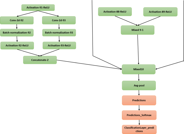
Complex building blocks (inception blocks) are introduced as models with the fewer numbers of parameters and higher efficiency of the training process by replacing the fully connected architectures with sparsely connected architectures. The network has been built from convolutional building blocks called inception modules, which are stacked on top of each other. Each inception module consists of a combination of convolutional layers with kernel sizes of 1×1, 3×3, and 5×5, which their output filter banks concatenated into a single output vector that will be the input of the next stage. 1×1 convolutions in each inception module is used for dimensionality reduction before applying computationally expensive 3×3 and 5×5 convolutions. Factorization of convolutions into smaller convolutions results in aggressive dimension reduction inside the network, which leads to the fewer numbers of parameters and low computational cost. Inception models are trained using stochastic gradient descent. Batch size is chosen as 32 for 100 epochs and momentum with the decay of 0.9. Learning rate is initialized by 0.045 and decayed every second epoch by the exponential rate of 0.94 [37, 38]. Pre-trained Inception-v3 is used in our experiments. The inception models are updated in this version of the network to further boost ImageNet classification accuracy. The last part of the network, which is used for fine-tuning in our experiments is shown in Fig. 4.

Fig. 4.

Last layers of the Inception-v3 architecture.

2.3. Training and validation

In our experiments, the total of 3149 different tissues are extracted from OCT pullback images and are manually labeled as calcification, fibrosis, normal intima, macrophage, media, and neovascularization. Annotated images are validated by expert cardiologists. the ROIs are extracted from each frame of the sequence using the manual segmentation and they are labeled as 1 to 6 for calcification, fibrosis, normal intima, macrophage, media, and neovascularization respectively. To start the experiments, 66% of the ROIs are selected randomly as the training set. To avoid any correlation between training, test, and validation sets, 50% of the remaining ROIs are randomly selected as the validation set and the test set is built on the last residual ROIs. The experiments are performed in four different steps to find the optimal tissue characterization framework.

2.3.1. Classification using fine-tuned networks

For each convolutional neural network, before starting the training process, fine-tuning is performed as follows: Considering that the number of nodes in the last fully connected layer depends on the number of classes in each dataset, for the first step, we removed the classification layers and replaced them by the layers, which are designed appropriately for our classification task. The iterative weight update in any convolutional neural network is performed by random weight initialization at each layer of the network. Since the number of labeled data is limited in our experiments, weight initialization can be performed using the weights of the pre-trained networks. Therefore, iterative weight updates of equations 2 and 3 lead to a fast convergence to find the desirable local minimum for the cost function (equation 1). Therefore, for the next step, the weights are initialized at each layer of the network with the weights of the pre-trained network. The iterative weight update can be started using layer-wise fine-tuning by finding the optimal learning parameters at each convolutional and fully connected layer. Considering the complexity of the pathological formations, the process of fine-tuning the pre-trained AlexNet is performed based on our new dataset. The last three layers of the pre-trained network (fc8, prob, and classification layer) are replaced by a set of layers, which are designed for multi-class classification task to classify calcification, fibrosis, macrophage, neovascularization, and normal tissues (intima, and media). The values of µ and γ are kept at 0.9 and 0.95 respectively and the learning rate for the last fully connected layers (fc6, fc7, and fc8) is set to 0.1 to learn faster in the last layers and we started decreasing the learning rates to 0.01 from the last convolutional layer (Conv5).

Since by adding convolutional layers and reducing the size of the filters, we will have access to detailed image information, increasing the depth and width of the network can improve the quality of the network architecture. To have a fair comparison among the performance of pre-trained networks, we selected VGG-19 from the category of very deep CNN architectures, which is the last modified version of this category. As it is explained in the previous section, VGG-19 has almost the same configuration of the AlexNet with more convolutional layers and smaller filter sizes. Therefore, fine-tuning the VGG-19 is performed using the same strategy that is applied to AlexNet. We started fine-tuning by removing the classification layers (fc8, prob, and output) and replacing them by a set of layers, which are appropriate for multi-class classification of various coronary artery tissues (calcification, fibrosis, macrophage, neovascularization, normal intima, and media). We started fine-tuning from the last fully connected layer (fc8) and increase the depth of fine-tuning gradually by evaluating the network performance at each fine-tuning level. To find the optimal parameters at each level of fine-tuning, an interval of values close to the optimal values of fine-tuned AlexNet is chosen. For all the networks applied in this study, the optimal parameters are determined by grid searching for the defined interval of values and evaluating the performance of the network at each step. The best performance of the network obtained by assigning fixed values of 0.8, and 0.85 to µ and γ respectively. The learning rate is determined as 0.2 for the last fully connected layers (fc6, fc7, and fc8) and is decreased to 0.01 from the last convolutional layer (Conv5-4).

Complex building blocks are very deep network architectures, which use the particular configuration of inception modules to reduce the number of parameters and consequently improve the efficiency of the training procedure. We selected Inception-v3 from the category of complex network architectures to perform our experiments because in the latest versions of inception models, factorization into smaller convolutions is performed. Therefore, each 5×5 convolution is replaced by two 3×3 convolutions in the latest versions such as inception-v3. Also, in this version, the grid sizes between the inception blocks are reduced, which results in reducing the computational cost and fast training the network. Considering the complexity of the Inception architectures, changing the network can interfere with computational gains. Therefore, it is more difficult to adapt these types of networks to a new classification task. To fine-tune the network, we removed the last layers of the network (predictions, predictions-softmax, and ClassificationLayer-predictions), which aggregates the extracted features from the network for classification task and added a new set of classification layers adapted to our data set to the network graph. The new layers are connected to the transferred network graph and the learning rate for the fully connected layer is set to 0.1.

At each step of fine-tuning for all the networks, the accuracy is calculated on the validation set and the training process is stopped when the highest accuracy on the validation set is obtained. By terminating the training process, classification is performed on the test set using each fine-tuned network separately.

2.3.2. Training random forest using deep features generated by pre-trained networks

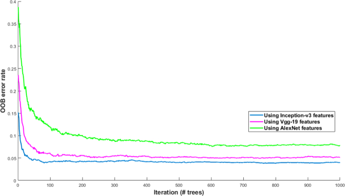
In this experiment, pre-trained networks are used as feature generators. The activations extracted from the last layer before classification layer is used to train Random Forest to classify various coronary artery tissues. Using AlexNet, and VGG-19, features are extracted from the last fully connected layer right before the classification layer (fc7). Each feature vector represents 4096 attributes of the labeled tissue. Using Inception-v3, features are extracted from the last depth concatenation layer (mixed10). Each feature vector represents 131072 attributes of the labeled tissue. It is demonstrated in our previous work that Random Forest is a robust classifier with quick training process and low risk of overfitting [49]. It works based on generating an ensemble of trees. The trees are grown based on the CART methodology to maximum size without pruning. Generalization error for Random Forest classifier is proportional to the ratio ρ/s², which (s) and (ρ) are respectively defined as the strength of the trees and correlation between them. the smaller this ratio results in the better performance of Random Forest [50, 51]. To find the optimal number of trees, The performance of Random Forest is evaluated for 1000 of trees while it is trained on each set of features extracted from each network separately. The OOB error rate is stopped decreasing when the tree number is assigned to 250 using the features extracted from Inception-v3, and VGG-19, and 300 using the features extracted from AlexNet (see Fig. 5). The fewer number of trees accelerates the training process by reducing the computational complexity. The number of randomly selected predictors (m_try) is set to 7.

Fig. 5.

OOB error rate is calculated to find the optimal number of trees to train Random Forest model. The performance of Random Forest is evaluated by calculating OOB errors while it is trained on each set of features extracted from each network separately. The OOB error rate is calculated for 1000 of trees.

Training features extracted from each pre-trained network and used separately to train Random Forest. Classification is performed on the test set using the test features extracted by each pre-trained network.

2.3.3. Classification using majority voting

Inspired by the ensemble learning approaches, we applied weighted majority voting (equation 4) on the classification results obtained by the second experiment. Classification is performed by Random Forest using the features extracted from AlexNet, VGG-19, and Inception-v3.

$$C(x)={\mathit{\text{argmax}}}_i{\displaystyle \sum _j{w}_{j}I(C_j(x)=i),}$$ (4)

where C(x) is the classification label with the majority vote, i is the class label (it can be varying from 1 to 6 for calcification, fibrosis, normal intima, macrophage, media, and neovascularization), w_j is the weight of j^th tissue label and I is the indicator function. Thus, majority voting is applied to search in all the classification labels for the most frequent label assigned to each tissue using equation 5.

$$C(x)=\mathit{\text{mode}}\{C_1(x),C_2(x),C_3(x)\},$$ (5)

where C₁(x), C₂(x), and C₃(x) are Random Forest classification results using the features extracted from AlexNet, VGG-19, and Inception-v3 respectively. weights are set to 1/3 for all the three sets of classification results except those which are predicted with three different tissue labels, C₁(x) ≠ C₂(x) ≠ C₃(x). Because for each tissue, we can get different information of that particular tissue using each network separately, which may be significant in proper characterization of the tissues. Regardless the overall performance of each network, AlexNet works very well to characterize normal intima and VGG-19 gives us important information regarding the calcification. Therefore, except the situation that the model should take the best decision between three different labels to choose the one, which has higher probability to belong to the true class label, we decided to look for more frequent label as the majority vote in other cases. Since the mode of C₁(x), C₂(x), and C₃(x) when C₁(x) ≠ C₂(x) ≠C₃(x) gives us the smallest tissue label as the majority vote, we put more weight on the third group of predicted labels if C₁(x) ≠ C₂(x) ≠C₃(x) considering the strength of deep Inception-v3 features. Therefore, the majority vote will be on the class label with the highest probability of belonging to the true class label.

2.3.4. RF classification using deep feature fusion

To consider all possible ways to find the optimal tissue characterization framework, we combined the features obtained from AlexNet, and VGG-19 to train Random Forest. Classification is performed on the test set and the results are compared against the previous experiments. The features extracted from Inception-v3 are not used in this experiment since the size of the feature matrix is huge to be combined with other feature matrices.

Matlab 2017b is used for all the experiments in this study. The computer configuration is as follows: Intel core i7-6700k, 16GB of RAM. The experiments are performed on GPU (GForce Tiran X, RAM: 12GB), Windows 10 (64 bit).

3. Results

3.1. Classification using fine-tuned networks

For the first experiment, fine-tuning is performed on AlexNet, VGG-19, and Inception-v3 from different categories of simple architectures, very deep architectures, and complex networks respectively. The optimal fine-tuning parameters are estimated and the networks are trained by assigning the new learning parameters. Classification is performed by each network separately and accuracy, sensitivity, and specificity are measured using the corresponding confusion matrix for each network. The results are shown in Figs. 6–8, and Tables 2–4.

Fig. 6.

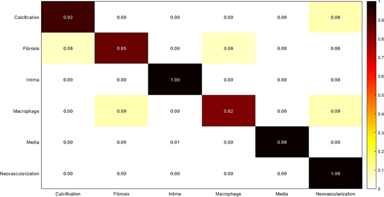
Confusion matrix of intracoronary tissue classification using fine-tuned AlexNet.

Fig. 7.

Confusion matrix of intracoronary tissue classification using fine-tuned VGG-19.

Fig. 8.

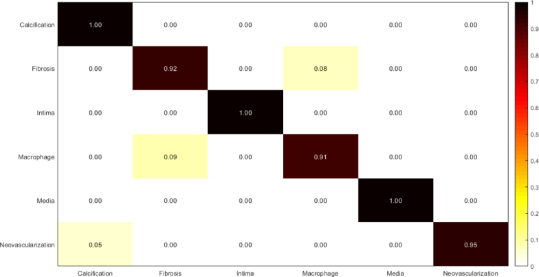
Confusion matrix of intracoronary tissue classification using fine-tuned Inception-v3.

Table 2.

Measured sensitivity, specificity, and accuracy of tissue classification using fine-tuned AlexNet.

Tissue	Accuracy	Sensitivity	Specificity
Calcification	0.95	0.92	0.99
Fibrosis	0.92	0.85	0.99
Normal intima	1.00	1.00	1.00
Macrophage	0.89	0.82	0.97
Media	1.00	0.99	1.00
Neovascularization	0.98	1.00	0.97

Table 3.

Measured sensitivity, specificity, and accuracy of tissue classification using fine-tuned VGG-19.

Tissue	Accuracy	Sensitivity	Specificity
Calcification	0.95	0.92	0.99
Fibrosis	1.00	1.00	1.00
Normal intima	1.00	1.00	1.00
Macrophage	0.95	0.91	1.00
Media	1.00	1.00	1.00
Neovascularization	0.99	1.00	0.99

Table 4.

Measured sensitivity, specificity, and accuracy of tissue classification using fine-tuned Inception-v3.

Tissue	Accuracy	Sensitivity	Specificity
Calcification	1.00	1.00	1.00
Fibrosis	0.96	0.92	0.99
Normal intima	1.00	1.00	1.00
Macrophage	0.95	0.91	0.99
Media	1.00	1.00	1.00
Neovascularization	0.97	0.95	1.00

The results of the experiments demonstrate the higher performance of VGG-19 and Inception-v3 compared against AlexNet, which was expected considering the deep structure of VGG-19, and Inception-v3 architectures. Although using pre-trained networks reduce the computational burden, which results in reducing the training time and convergence issues, but a considerable amount of time is still required to find the optimal learning parameters and retrain the fine-tuned networks (approximately two hours for each network). Also, there is a risk of overfitting in deep fine-tuning a network. The following steps are proposed to find the optimal tissue characterization model, which can overcome the mentioned issues in an efficient way.

3.2. Training random forest using deep features generated by pre-trained networks

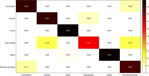
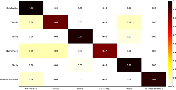
In this experiment, deep features are extracted from AlexNet, VGG-19, and Inception-v3. By applying each network separately as feature generator, the training features are extracted to train Random Forest and the classification is performed on the test set. Features are extracted from the last fully connected layer before the classification layer (fc7) in AlexNet, and VGG-19 architectures, and the last depth concatenation layer (mixed10) in Inception-v3 architecture. Accuracy, sensitivity, and specificity are measured using the corresponding confusion matrix for each classification result, which are shown in Figs. 9–11, and Tables 5–7.

Fig. 9.

Confusion matrix of intracoronary tissue classification: Random Forest is trained using the deep features extracted from AlexNet.

Fig. 10.

Confusion matrix of intracoronary tissue classification: Random Forest is trained using the deep features extracted from VGG-19.

Fig. 11.

Confusion matrix of intracoronary tissue classification: Random Forest is trained using the deep features extracted from Inception-v3.

Table 5.

Measured sensitivity, specificity, and accuracy of tissue classification using RF. Features are extracted from AlexNet.

Tissue	Accuracy	Sensitivity	Specificity
Calcification	0.95	0.92	0.98
Fibrosis	0.95	0.92	0.99
Normal intima	0.99	1.00	1.00
Macrophage	0.80	0.64	0.95
Media	0.99	1.97	1.00
Neovascularization	0.92	1.89	0.95

Table 6.

Measured sensitivity, specificity, and accuracy of tissue classification using RF. Features are extracted from VGG-19.

Tissue	Accuracy	Sensitivity	Specificity
Calcification	1.00	1.00	1.00
Fibrosis	0.92	0.85	0.99
Normal intima	0.98	0.97	0.99
Macrophage	0.91	0.82	1.00
Media	0.98	0.97	0.98
Neovascularization	0.97	0.95	1.00

Table 7.

Measured sensitivity, specificity, and accuracy of tissue classification using RF. Features are extracted from Inception-v3.

Tissue	Accuracy	Sensitivity	Specificity
Calcification	0.90	0.83	0.97
Fibrosis	0.95	0.92	0.99
Normal intima	0.95	0.91	0.98
Macrophage	0.90	0.82	0.99
Media	0.96	0.94	0.98
Neovascularization	0.96	0.95	0.97

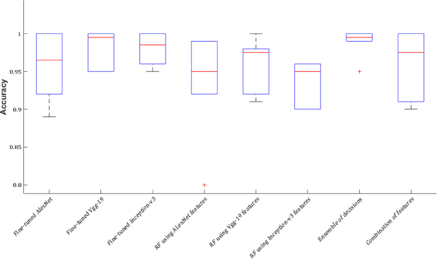
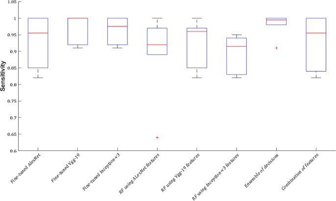
Regardless of the time, which is spent to find the optimal learning parameters, the process of feature extraction from all the three networks, and training the Random Forest using each set of features takes approximately twice less time than retraining a network. Using pre-trained networks as feature extractor overcomes the problems of fine-tuning, training time, and overfitting concerns. But, the classification performance is not as high as using CNNs as the classifiers (Figs. 14–16). To solve this problem, the following two experiments are performed and the results of all experiments compared against each other.

Fig. 14.

Accuracy is reported as the mean ± standard deviation of the measured accuracies for all the tissues in each experiment.

Fig. 16.

Specificity is reported as the mean ± standard deviation of the measured specificities for all tissues in each experiment.

3.3. Majority voting

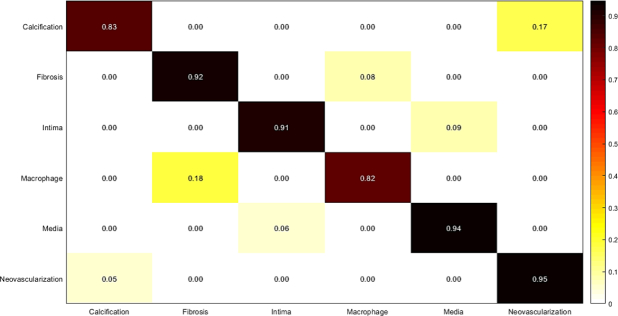
In this experiment, weighted majority voting is applied on Random Forest classification results using each set of features extracted from the three mentioned networks. The results are illustrated in Fig. 12, and Table 8. The results show a good improvement of accuracy, sensitivity, and specificity, which are calculated for the final classification using majority voting.

Fig. 12.

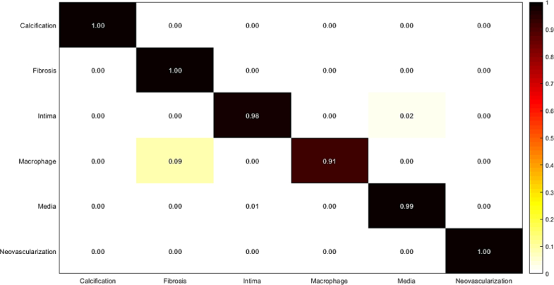
Confusion matrix of intracoronary tissue classification using majority voting approach.

Table 8.

Measured sensitivity, specificity, and accuracy of tissue classification using majority voting approach.

Tissue	Accuracy	Sensitivity	Specificity
Calcification	1.00	1.00	1.00
Fibrosis	1.00	1.00	1.00
Normal intima	0.99	0.98	1.00
Macrophage	0.95	0.91	1.00
Media	0.99	0.99	1.00
Neovascularization	1.00	1.00	1.00

3.4. RF classification using deep feature fusion

In this experiment, we combined deep features extracted from AlexNet, and VGG-19 to train Random Forest. The results are shown in Fig. 13 and Table 9. The results of the last two experiments show that majority voting approach performs better than Random Forest classification result while it is trained on the combination of features.

Fig. 13.

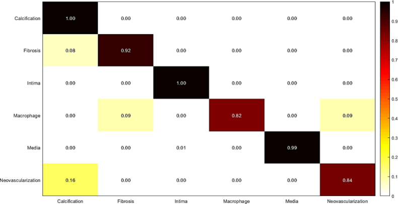
Confusion matrix of intracoronary tissue classification using RF: Combination of features extracted from pre-trained AlexNet, and VGG-19 are used to train Random Forest.

Table 9.

Measured sensitivity, specificity, and accuracy of tissue classification: Combination of features extracted from pre-trained AlexNet, and VGG-19 are used to train Random Forest.

Tissue	Accuracy	Sensitivity	Specificity
Calcification	1.00	1.00	1.00
Fibrosis	0.96	0.92	1.00
Normal intima	1.00	1.00	1.00
Macrophage	0.90	0.82	0.98
Media	0.99	0.99	1.00
Neovascularization	0.91	0.84	0.98

CNN features are very strong to describe various pathological formations and tissues, and the results of the experiments are high due to the classification of ROIs. Therefore, to choose the optimal tissue characterization model considering all the experiments, and to compare the results of the experiments against each other, the mean ± standard deviation of the values of accuracy, sensitivity, and specificity obtained for all the tissues performing each experiment are calculated and the results are shown in Figs. 14–16 and Table 10. Although the combination of features can improve the classification results compared against using each network separately as feature extractor, the results of majority voting approach are considerably higher than the classification results using the combination of features (Figs. 14–16).

Fig. 15.

Sensitivity is reported as the mean ± standard deviation of the measured sensitivities for all tissues in each experiment.

Table 10.

Accuracy, sensitivity, and specificity obtained from each experiment. The accuracy, sensitivity, and specificity are reported as the mean ± standard deviation of the values of accuracy, sensitivity, and specificity obtained for all the tissues performing each experiment.

Tissue	Accuracy	Sensitivity	Specificity
Fine-tuned AlexNet	0.96±0.04	0.92±0.08	0.99±0.01
Fine-tuned VGG-19	0.98±0.02	0.97±0.03	1.00±0.00
Fine-tuned Inception-v3	0.98±0.02	0.96±0.04	1.00±0.00
RF(AlexNet features)	0.93±0.07	0.89±0.13	0.98±0.02
RF(VGG-19 features)	0.96±0.04	0.92±0.07	0.99±0.01
RF(Inception-v3 features)	0.94±0.03	0.90±0.06	0.98±0.01
Majority voting RF	0.99±0.01	0.98±0.02	1.00±0.00
RF(combination of features)	0.94±0.06	0.90±0.10	0.99±0.01

4. Discussion

In this study, the performance of pre-trained networks is discussed. Three different state-of-the-art networks (AlexNet, VGG-19, and Inception-v3) are used in four different experiments. The experiments started with fine-tuning the networks and using them for tissue classification of six different tissue labels (calcification, fibrosis, neovascularization, macrophage, normal intima, and media). We started with fine-tuning the networks, which is the most common way of applying pre-trained networks for various applications in the field of medical image analysis. Each experiment is designed based on the limitations of the previous experiment to achieve the main goal of this study, which defined as designing an accurate intracoronary tissue classification model using deep feature learning in an efficient procedure. The second experiment is performed to avoid convergence issues in fine-tuning the networks, overfitting by deep fine-tuning the networks, and training time. Deep features are very strong to describe arterial tissues and Random Forest works efficiently on large datasets with a very low risk of overfitting. Also, the training process is considerably fast using Random Forest. But, when pre-trained networks are used as feature generators without fine-tuning, the classification results show lower accuracy, sensitivity, and specificity compared against using fine-tuned networks as classifiers. Majority voting on classification results of Random Forest can considerably improve the results of the second experiment without adding a huge computational burden. The accuracy, sensitivity, and specificity obtained from the third experiment (majority voting from Random Forest classification) can compete against the classification performance of the fine-tuned networks.

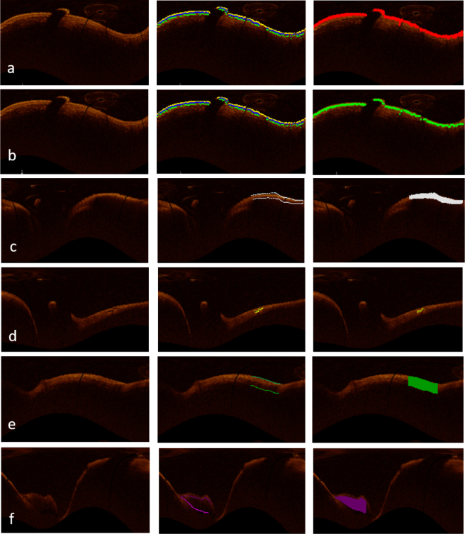
By evaluating the results of all the experiments, it is more efficient if we use pre-trained networks as feature extractors and train Random Forest for each set of generated features to perform the classification. Then, majority voting method provides the final tissue classification result. Fig. 17 shows classification results for each coronary artery tissue. The results of the experiments are high due to the classification of ROIs. The optimal model is based on extracting features from pre-trained networks without any fine-tuning, and train Random Forest as the classifier. Also, Random Forest is known as a classifier with the low risk of overfitting. However, to overcome the concern of overfitting, leave-one-out cross-validation is performed by leaving out the OCT images of one patient for test set and training the classifier on the OCT images of the remaining patients at each step of the experiment (Fig. 18).

Fig. 17.

From left to right: The first image shows the original OCT image in planar representation, manual segmentation for each tissue is illustrated in the second image, and the third image is the classification result, which is shown for intima in (a), media in (b), fibrosis in (c), neovascularization in (d), macrophage in (e), and calcification in (f).

Fig. 18.

Leave-one-out cross-validation using pre-trained networks as feature extractor and majority voting for final classification results. The experiments were performed 33 times and each time, one patient was left out for test set and the classifier was trained on the OCT images of the remaining patients. Measured accuracies obtained from all the patients are sorted from lower to higher accuracy.

The experiments performed by one random selection of training, validation, and test sets to reduce the computational burden. To evaluate the performance of the model using various randomizations of the training, validation, and test sets, we performed the experiments for 10 iterations using the final characterization model (feature extraction using CNNs, classification using RF, and final classification result by majority voting). As it is shown in Table 11, although there are some variations between the results obtained from each iteration because of different selections of training, validation, and test sets, but the accuracy, sensitivity, and specificity of the tissue characterization demonstrate the robustness of the model to characterize between different coronary artery tissues.

Table 11.

Measured sensitivity, specificity, and accuracy of tissue classification: Using the final model (feature extraction using CNNs, classification using RF, and final classification result by majority voting), we perform the experiment in 10 iterations to evaluate the performance of the model using various randomization of the training, validation, and test sets. The accuracy, sensitivity, and specificity are reported as the mean ± std for all the iterations.

Tissue	Accuracy	Sensitivity	Specificity
Calcification	0.95±0.05	0.91±0.08	0.98±0.02
Fibrosis	0.95±0.04	0.91±0.07	0.98±0.02
Normal intima	1.00±0.00	1.00±0.00	1.00±0.00
Macrophage	0.91±0.06	0.84±0.10	0.99±0.01
Media	1.00±0.00	1.00±0.00	1.00±0.00
Neovascularization	0.98±0.02	0.97±0.03	0.99±0.01

5. Conclusion

The goal of this study was to propose a new approach for OCT imaging using deep feature learning from different CNN models and to evaluate their performance on a complex multi-class classification problem such as pathological formations in coronary artery tissues. The most significant outcome is to be able to automatically differentiate between intracoronary pathological formations observed from OCT imaging. This might be highly relevant for the automatic assessment of coronary artery disease in KD. Majority voting from Random Forest classification using deep features have been successful in classifying coronary artery tissues. The final tissue labels were obtained with high accuracy, sensitivity, and specificity, which confirm the robustness of our proposed technique considering the high variability of pathological formations, OCT artifacts, and the small size of the arteries in pediatric patients, which is followed by very thin layers in coronary artery structure. In this work, we have outlined the relevance of deep features obtained using transfer learning for OCT imaging and the practical aspect of using RF classification to obtain the final decision in a clinically acceptable computational time. For future works, we will focus on detecting intimal hyperplasia by measuring the thickness of intima, and severity of pathological formations by evaluating distensibility variations as a result of calcification, and fibrous scarring. With the proper dataset and manual annotation, this might be adapted for adult coronary artery diseases to fully assess the structural information of the coronary artery.

Funding

Fonds de Recherche du Québec-Nature et technologies.

Disclosures

The authors declare that there are no conflicts of interest related to this article.

References

- 1.Newburger J. W., Takahashi M., Gerber M. A., Gewitz M. H., Tani L. Y., Burns J. C., Shulman S. T., Bolger A. F., Ferrieri P., Baltimore R. S., et al. , “Diagnosis, treatment, and long-term management of Kawasaki disease,” Circulation 110, 2747–2771 (2004). 10.1161/01.CIR.0000145143.19711.78 [DOI] [PubMed] [Google Scholar]
- 2.Hauser M., Bengel F., Kuehn A., Nekolla S., Kaemmerer H., Schwaiger M., Hess J., “Myocardial blood flow and coronary flow reserve in children with normal epicardial coronary arteries after the onset of Kawasaki disease assessed by positron emission tomography,” Pediatr. Cardiol. 25, 108–112 (2004). 10.1007/s00246-003-0472-9 [DOI] [PubMed] [Google Scholar]
- 3.Orenstein J. M., Shulman S. T., Fox L. M., Baker S. C., Takahashi M., Bhatti T. R., Russo P. A., Mierau G. W., de Chadarévian J. P., Perlman E. J., et al. , “Three linked vasculopathic processes characterize Kawasaki disease: a light and transmission electron microscopic study,” PloS one 7, e38998 (2012). 10.1371/journal.pone.0038998 [DOI] [PMC free article] [PubMed] [Google Scholar]
- 4.Dionne A., Ibrahim R., Gebhard C., Bakloul M., Selly J.-B., Leye M., Déry J., Lapierre C., Girard P., Fournier A., et al. , “Coronary wall structural changes in patients with Kawasaki disease: new insights from optical coherence tomography (OCT),” J. Am. Hear. Assoc. 4, e001939 (2015). [DOI] [PMC free article] [PubMed] [Google Scholar]
- 5.Baim D. S., Grossman W., Cardiac Catheterization, Angiography, and Intervention (Lippincott Williams & Wilkins, 1996). [Google Scholar]
- 6.Kitabata H., Akasaka T., “Visualization of plaque neovascularization by oct,” in Optical Coherence Tomography, (InTech, 2013). 10.5772/53051 [DOI] [Google Scholar]
- 7.Jang I.-K., Bouma B. E., Kang D.-H., Park S.-J., Park S.-W., Seung K.-B., Choi K.-B., Shishkov M., Schlendorf K., Pomerantsev E., et al. , “Visualization of coronary atherosclerotic plaques in patients using optical coherence tomography: comparison with intravascular ultrasound,” J. Am. Coll. Cardiol. 39, 604–609 (2002). 10.1016/S0735-1097(01)01799-5 [DOI] [PubMed] [Google Scholar]
- 8.Fujii K., Kawasaki D., Masutani M., Okumura T., Akagami T., Sakoda T., Tsujino T., Ohyanagi M., Masuyama T., “Oct assessment of thin-cap fibroatheroma distribution in native coronary arteries,” JACC: Cardiovasc. Imaging 3, 168–175 (2010). [DOI] [PubMed] [Google Scholar]
- 9.Taguchi Y., Itoh T., Oda H., Uchimura Y., Kaneko K., Sakamoto T., Goto I., Sakuma M., Ishida M., Terashita D., et al. , “Coronary risk factors associated with OCT macrophage images and their response after CoCr everolimus-eluting stent implantation in patients with stable coronary artery disease,” Atherosclerosis 265, 117–123 (2017). 10.1016/j.atherosclerosis.2017.08.002 [DOI] [PubMed] [Google Scholar]
- 10.Swirski F. K., Robbins C. S., Nahrendorf M., “Development and function of arterial and cardiac macrophages,” Trends Immunol. 37, 32–40 (2016). 10.1016/j.it.2015.11.004 [DOI] [PMC free article] [PubMed] [Google Scholar]
- 11.Liu W., Zhang Y., Yu C.-M., Ji Q.-W., Cai M., Zhao Y.-X., Zhou Y.-J., “Current understanding of coronary artery calcification,” J. Geriatric Cardiology: JGC 12, 668 (2015). [DOI] [PMC free article] [PubMed] [Google Scholar]
- 12.Madhavan M. V., Tarigopula M., Mintz G. S., Maehara A., Stone G. W., Généreux P., “Coronary artery calcification: pathogenesis and prognostic implications,” J. Am. Coll. Cardiol. 63, 1703–1714 (2014). 10.1016/j.jacc.2014.01.017 [DOI] [PubMed] [Google Scholar]
- 13.J. J. W. Group et al. , “Guidelines for diagnosis and management of cardiovascular sequelae in Kawasaki disease (JCS 2008),” Circulation J. 74, 1989–2020 (2010). 10.1253/circj.CJ-10-74-0903 [DOI] [PubMed] [Google Scholar]
- 14.Kawasaki M., Takatsu H., Noda T., Sano K., Ito Y., Hayakawa K., Tsuchiya K., Arai M., Nishigaki K., Takemura G., et al. , “In vivo quantitative tissue characterization of human coronary arterial plaques by use of integrated backscatter intravascular ultrasound and comparison with angioscopic findings,” Circulation 105, 2487–2492 (2002). 10.1161/01.CIR.0000017200.47342.10 [DOI] [PubMed] [Google Scholar]
- 15.Rathod K. S., Hamshere S. M., Jones D. A., Mathur A., “Intravascular ultrasound versus optical coherence tomography for coronary artery imaging–apples and oranges,” Interv. Cardiol. Rev. 10, 8–15 (2015). [DOI] [PMC free article] [PubMed] [Google Scholar]
- 16.Bezerra H. G., Costa M. A., Guagliumi G., Rollins A. M., Simon D. I., “Intracoronary optical coherence tomography: a comprehensive review: clinical and research applications,” JACC: Cardiovasc. Interv. 2, 1035–1046 (2009). [DOI] [PMC free article] [PubMed] [Google Scholar]
- 17.Boudoux C., Fundamentals of Biomedical Optics (Pollux, 2016). [Google Scholar]
- 18.Drexler W., Fujimoto J. G., Optical Coherence Tomography: Technology and Applications (Springer, 2015). 10.1007/978-3-319-06419-2 [DOI] [Google Scholar]
- 19.Xu C., Schmitt J. M., Carlier S. G., Virmani R., “Characterization of atherosclerosis plaques by measuring both backscattering and attenuation coefficients in optical coherence tomography,” J. Biomed. Opt. 13, 034003 (2008). 10.1117/1.2927464 [DOI] [PubMed] [Google Scholar]
- 20.Van Soest G., Regar E., KoljenoviÄ S., van Leenders G. L., Gonzalo N., van Noorden S., Okamura T., Bouma B. E., Tearney G. J., Oosterhuis J. W., et al. , “Atherosclerotic tissue characterization in vivo by optical coherence tomography attenuation imaging,” J. Biomed. Opt 15, 011105 (2010). 10.1117/1.3280271 [DOI] [PubMed] [Google Scholar]
- 21.Ughi G. J., Adriaenssens T., Sinnaeve P., Desmet W., hooge J. D, “Automated tissue characterization of in vivo atherosclerotic plaques by intravascular optical coherence tomography images,” Biomed. Opt. Express 4, 1014–1030 (2013). 10.1364/BOE.4.001014 [DOI] [PMC free article] [PubMed] [Google Scholar]
- 22.Gargesha M., Shalev R., Prabhu D., Tanaka K., Rollins A. M., Costa M., Bezerra H. G., Wilson D. L., “Parameter estimation of atherosclerotic tissue optical properties from three-dimensional intravascular optical coherence tomography,” J. Med. Imaging 2, 016001 (2015). 10.1117/1.JMI.2.1.016001 [DOI] [PMC free article] [PubMed] [Google Scholar]
- 23.Macedo M. M., Nicz P. F., Campos C. M., Lemos P. A., Gutierrez M. A., “Spatial-frequency approach to fibrous tissue classification in intracoronary optical images,” in Computing in Cardiology Conference (CinC), 2016, (IEEE, 2016), pp. 477–480. [Google Scholar]
- 24.Gan Y., Tsay D., Amir S. B., Marboe C. C., Hendon C. P., “Automated classification of optical coherence tomography images of human atrial tissue,” J. Biomed. Opt. 21, 101407 (2016). 10.1117/1.JBO.21.10.101407 [DOI] [PMC free article] [PubMed] [Google Scholar]
- 25.Rico-Jimenez J. J., Campos-Delgado D. U., Villiger M., Otsuka K., Bouma B. E., Jo J. A., “Automatic classification of atherosclerotic plaques imaged with intravascular oct,” Biomed. Opt. Express 7, 4069–4085 (2016). 10.1364/BOE.7.004069 [DOI] [PMC free article] [PubMed] [Google Scholar]
- 26.Lo S.-C., Lou S.-L., Lin J.-S., Freedman M. T., Chien M. V., Mun S. K., “Artificial convolution neural network techniques and applications for lung nodule detection,” IEEE Transactions on Med. Imaging 14, 711–718 (1995). 10.1109/42.476112 [DOI] [PubMed] [Google Scholar]
- 27.Hochreiter S., Schmidhuber J., “Long short-term memory,” Neural Comput. 9, 1735–1780 (1997). 10.1162/neco.1997.9.8.1735 [DOI] [PubMed] [Google Scholar]
- 28.Eigen D., Rolfe J., Fergus R., LeCun Y., “Understanding deep architectures using a recursive convolutional network,” arXiv preprint arXiv:1312.1847 (2013).
- 29.Zeiler M. D., Fergus R., “Visualizing and understanding convolutional networks,” in European Conference on Computer Vision, (Springer, 2014), pp. 818–833. [Google Scholar]
- 30.Simonyan K., Zisserman A., “Very deep convolutional networks for large-scale image recognition,” arXiv preprint arXiv:1409.1556 (2014).
- 31.Szegedy C., Liu W., Jia Y., Sermanet P., Reed S., Anguelov D., Erhan D., Vanhoucke V., Rabinovich A., “Going deeper with convolutions,” in Proceedings of the IEEE Conference on Computer Vision and Pattern Recognition, (2015), pp. 1–9. [Google Scholar]
- 32.Roth H. R., Farag A., Lu L., Turkbey E. B., Summers R. M., “Deep convolutional networks for pancreas segmentation in CT imaging,” in SPIE Medical Imaging, (International Society for Optics and Photonics, 2015), pp. 94131G. [Google Scholar]
- 33.Ciompi F., de Hoop B., van Riel S. J., Chung K., Scholten E. T., Oudkerk M., de Jong P. A., Prokop M., van Ginneken B., “Automatic classification of pulmonary peri-fissural nodules in computed tomography using an ensemble of 2D views and a convolutional neural network out-of-the-box,” Med. Image Analysis 26, 195–202 (2015). 10.1016/j.media.2015.08.001 [DOI] [PubMed] [Google Scholar]
- 34.Havaei M., Davy A., Warde-Farley D., Biard A., Courville A., Bengio Y., Pal C., Jodoin P.-M., Larochelle H., “Brain tumor segmentation with deep neural networks,” Med. Image Analysis 35, 18–31 (2016). [DOI] [PubMed] [Google Scholar]
- 35.Krizhevsky A., Sutskever I., Hinton G. E., “Imagenet classification with deep convolutional neural networks,” in Advances in Neural Information Processing Systems, (2012), pp. 1097–1105. [Google Scholar]
- 36.Litjens G., Kooi T., Bejnordi B. E., Setio A. A. A., Ciompi F., Ghafoorian M., van der Laak J. A., van Ginneken B., Sánchez C. I., “A survey on deep learning in medical image analysis,” Med. Image Analysis 42, 60–88 (2017). 10.1016/j.media.2017.07.005 [DOI] [PubMed] [Google Scholar]
- 37.Szegedy C., Vanhoucke V., Ioffe S., Shlens J., Wojna Z., “Rethinking the inception architecture for computer vision,” in Proceedings of the IEEE Conference on Computer Vision and Pattern Recognition, (2016), pp. 2818–2826. [Google Scholar]
- 38.Szegedy C., Liu W., Jia Y., Sermanet P., Reed S., Anguelov D., “Going deeper with convolutions,” in Proceedings of the IEEE conference on Computer Vision and Pattern Recognition, pp. 1–9. [Google Scholar]
- 39.Antony J., McGuinness K., O’Connor N. E., Moran K., “Quantifying radiographic knee osteoarthritis severity using deep convolutional neural networks,” in Pattern Recognition (ICPR), 2016 23rd International Conference on, (IEEE, 2016), pp. 1195–1200. [Google Scholar]
- 40.Gulshan V., Peng L., Coram M., Stumpe M. C., Wu D., Narayanaswamy A., Venugopalan S., Widner K., Madams T., Cuadros J., et al. , “Development and validation of a deep learning algorithm for detection of diabetic retinopathy in retinal fundus photographs,” JAMA 316, 2402–2410 (2016). 10.1001/jama.2016.17216 [DOI] [PubMed] [Google Scholar]
- 41.Esteva A., Kuprel B., Novoa R. A., Ko J., Swetter S. M., Blau H. M., Thrun S., “Dermatologist-level classification of skin cancer with deep neural networks,” Nature 542, 115 (2017). 10.1038/nature21056 [DOI] [PMC free article] [PubMed] [Google Scholar]
- 42.Fang L., Cunefare D., Wang C., Guymer R. H., Li S., Farsiu S., “Automatic segmentation of nine retinal layer boundaries in OCT images of non-exudative AMD patients using deep learning and graph search,” Biomed. Opt. Express 8, 2732–2744 (2017). 10.1364/BOE.8.002732 [DOI] [PMC free article] [PubMed] [Google Scholar]
- 43.Roy A. G., Conjeti S., Karri S. P. K., Sheet D., Katouzian A., Wachinger C., Navab N., “Relaynet: retinal layer and fluid segmentation of macular optical coherence tomography using fully convolutional networks,” Biomed. Opt. Express 8, 3627–3642 (2017). 10.1364/BOE.8.003627 [DOI] [PMC free article] [PubMed] [Google Scholar]
- 44.Venhuizen F. G., van Ginneken B., Liefers B., van Asten F., Schreur V., Fauser S., Hoyng C., Theelen T., Sánchez C. I., “Deep learning approach for the detection and quantification of intraretinal cystoid fluid in multivendor optical coherence tomography,” Biomed. Opt. Express 9, 1545–1569 (2018). 10.1364/BOE.9.001545 [DOI] [PMC free article] [PubMed] [Google Scholar]
- 45.Ji Z., Chen Q., Niu S., Leng T., Rubin D. L., “Beyond retinal layers: a deep voting model for automated geographic atrophy segmentation in sd-OCT images,” Transl. Vis. Sci. & Technol. 7, 1–1 (2018). 10.1167/tvst.7.1.1 [DOI] [PMC free article] [PubMed] [Google Scholar]
- 46.Schlegl T., Waldstein S. M., Bogunovic H., Endstraßer F., Sadeghipour A., Philip A.-M., Podkowinski D., Gerendas B. S., Langs G., Schmidt-Erfurth U., “Fully automated detection and quantification of macular fluid in OCT using deep learning,” Ophthalmology 125, 549–558 (2018). 10.1016/j.ophtha.2017.10.031 [DOI] [PubMed] [Google Scholar]
- 47.Karri S. P. K., Chakraborty D., Chatterjee J., “Transfer learning based classification of optical coherence tomography images with diabetic macular edema and dry age-related macular degeneration,” Biomed. Opt. Express 8, 579–592 (2017). 10.1364/BOE.8.000579 [DOI] [PMC free article] [PubMed] [Google Scholar]
- 48.Gessert N., Heyder M., Latus S., Lutz M., Schlaefer A., “Plaque classification in coronary arteries from IVOCT images using convolutional neural networks and transfer learning,” arXiv preprint arXiv:1804.03904 (2018).
- 49.Abdolmanafi A., Duong L., Dahdah N., Cheriet F., “Deep feature learning for automatic tissue classification of coronary artery using optical coherence tomography,” Biomed. Opt. Express 8, 1203–1220 (2017). 10.1364/BOE.8.001203 [DOI] [PMC free article] [PubMed] [Google Scholar]
- 50.Criminisi A., Shotton J., Decision Forests for Computer Vision and Medical Image Analysis (Springer Science & Business Media, 2013). 10.1007/978-1-4471-4929-3 [DOI] [Google Scholar]
- 51.Kuhn M., Johnson K., Applied Predictive Modeling (Springer, 2013). 10.1007/978-1-4614-6849-3 [DOI] [Google Scholar]