Fully automatic multi‐organ segmentation for head and neck cancer radiotherapy using shape representation model constrained fully convolutional neural networks

Abstract

Purpose

Intensity modulated radiation therapy (IMRT) is commonly employed for treating head and neck (H&N) cancer with uniform tumor dose and conformal critical organ sparing. Accurate delineation of organs‐at‐risk (OARs) on H&N CT images is thus essential to treatment quality. Manual contouring used in current clinical practice is tedious, time‐consuming, and can produce inconsistent results. Existing automated segmentation methods are challenged by the substantial inter‐patient anatomical variation and low CT soft tissue contrast. To overcome the challenges, we developed a novel automated H&N OARs segmentation method that combines a fully convolutional neural network (FCNN) with a shape representation model (SRM).

Methods

Based on manually segmented H&N CT, the SRM and FCNN were trained in two steps: (a) SRM learned the latent shape representation of H&N OARs from the training dataset; (b) the pre‐trained SRM with fixed parameters were used to constrain the FCNN training. The combined segmentation network was then used to delineate nine OARs including the brainstem, optic chiasm, mandible, optical nerves, parotids, and submandibular glands on unseen H&N CT images. Twenty‐two and 10 H&N CT scans provided by the Public Domain Database for Computational Anatomy (PDDCA) were utilized for training and validation, respectively. Dice similarity coefficient (DSC), positive predictive value (PPV), sensitivity (SEN), average surface distance (ASD), and 95% maximum surface distance (95%SD) were calculated to quantitatively evaluate the segmentation accuracy of the proposed method. The proposed method was compared with an active appearance model that won the 2015 MICCAI H&N Segmentation Grand Challenge based on the same dataset, an atlas method and a deep learning method based on different patient datasets.

Results

An average DSC = 0.870 (brainstem), DSC = 0.583 (optic chiasm), DSC = 0.937 (mandible), DSC = 0.653 (left optic nerve), DSC = 0.689 (right optic nerve), DSC = 0.835 (left parotid), DSC = 0.832 (right parotid), DSC = 0.755 (left submandibular), and DSC = 0.813 (right submandibular) were achieved. The segmentation results are consistently superior to the results of atlas and statistical shape based methods as well as a patch‐wise convolutional neural network method. Once the networks are trained off‐line, the average time to segment all 9 OARs for an unseen CT scan is 9.5 s.

Conclusion

Experiments on clinical datasets of H&N patients demonstrated the effectiveness of the proposed deep neural network segmentation method for multi‐organ segmentation on volumetric CT scans. The accuracy and robustness of the segmentation were further increased by incorporating shape priors using SMR. The proposed method showed competitive performance and took shorter time to segment multiple organs in comparison to state of the art methods.

1. Introduction

Globally, there are an estimated 400,000–600,000 new head and neck (H&N) cancer cases, resulting in between 223,000 and 300,000 deaths per year.¹ Radiation therapy is one of the mainstay modalities for H&N treatment. Owing to the advance in shaping radiation dose for the morphologically complex H&N anatomy and pathology, intensity‐modulated radiation therapy (IMRT) has become the preferred radiotherapy method for H&N cancer. For instance, IMRT has been shown to significantly reduce the parotid dose, which is associated with a major long‐term side effect: dry mouth or xerostomia.² In inverse optimization, the organs‐at‐risk (OARs) sparing is achieved by penalizing doses to the correspondingly delineated volumes. Undersegmenting the OARs would expose them to unnecessarily high dose but oversegmenting the OARs could make optimization goals unattainable. Therefore, the effectiveness of IMRT depends on the accuracy of OAR segmentation, which is conventionally performed by oncologists and dosimetrists. However, the manual process is not only tedious but also introduces inconsistencies due to both inter‐patient and inter‐observer variabilities.³

To alleviate these problems, automated segmentation has been proposed. For it to be successfully applied to the H&N application, automated segmentation needs to tackle the inter‐patient variability and the large number of anatomical structures in a relatively small area, each presenting specific challenges, including relatively low CT soft tissue contrast and morphological complexity.⁴ The existing automatic H&N OARs segmentation methods can be broadly categorized as atlas or statistical shape‐appearance based methods.

The atlas method builds a library of OARs from manual segmentation and then extrapolates the library to a new patient via image registration.⁵ For H&N CT image segmentation, Han et al.⁵ employed a hierarchical atlas registration strategy. Urban et al.⁶ applied a random forest classifier that incorporates probabilistic atlas and image features of multimodal MRI images for the segmentation of H&N organs. Once an atlas is established on previously delineated patients, atlas methods can perform non‐supervised segmentation on a new patient. However, this method is sensitive to atlas selection and strongly depends on registration accuracy,⁷ making it a challenge to generalize.

In contrast to the atlas method, shape, or appearance statistical models based methods^{8, 9} delineate organs by restricting the final segmentation results to anatomically plausible shapes described by the statistical model.¹⁰ Conventional shape or appearance models based segmentation approaches are thus limited to the shape representation capacity of the statistical model, whose efficacy is diminished without impractically large training sets.¹⁰ To overcome the limitations of atlas and statistical appearance methods, multi atlas segmentation was augmented by an intensity model to improve segmentation accuracy. For instance, Fortunati et al.¹¹ combined atlas registration and intensity‐based classification to handle local variations of H&N OARs. Fritscher et al.¹⁰ enhanced multi atlas‐based segmentation by geodesic active contours and statistical appearance models for H&N CT images.

In recent years, deep learning based methods, particularly methods based on the convolutional neural network, have shown great promise in medical image segmentation. Applications include object or lesion classification,^{11, 12} organ or lesion detection,^{13, 14} organ and lesion segmentation,^{15, 16, 17} registration,¹⁸ and other tasks.^{18, 19, 20} Specifically, deep learning methods have been used for brain segmentation and achieved significantly better performance than conventional methods.^{21, 22, 23} In one of the few deep learning H&N OARs segmentation studies, Ibragimov et al.²⁴ modeled the task as multi‐segmentation sub‐tasks and trained 13 convolutional neural networks for the OARs. The trained networks were sequentially applied to patches of the test image in a sliding‐window fashion to locate the expected H&N OARs. After that, a Markov random field algorithm was used to refine the obtained classification results. Drawbacks of such patch‐based segmentation methods are redundant computation and inability to learn global features.²⁵ Wang, et al.²⁶ proposed a hierarchical vertex regression based segmentation model, which employed a novel learning‐based mechanism to locate critical model vertices. An iterative random‐forests framework was utilized to jointly learn shapes and appearance features. The model is computationally impractical, taking ~36 min to segment a single organ (brainstem) for a new subject. Its robustness is also affected by the accuracy of the shape correspondence detection method.

In this study, to further improve the accuracy and robustness of automated H&N segmentation, we integrate fully convolutional neural network (FCNN) and shape representation model (SRM) into a unified framework.

2. Materials and methods

In the unified framework, SRM is pre‐trained to learn the latent shape representation of the organs‐at‐risk (OARs). It is then employed as a regularizer in the training stage to enforce the predictions of the segmentation network for the H&N OARs anatomical properties. Specifically, the proposed framework is trained in the following steps: (a) train SRM using the labels of the training set to learn the latent shape representation of H&N OARs, which is employed to incorporate prior shape information into the segmentation network in the next step; (b) train the segmentation model, which combines FCNN and the pre‐trained SRM using 3D H&N CT scans with SRM parameters inherited from step 1. Once the network is trained, it is used to segment the H&N OARs of a new subject in a single forward pass.

2.A. Shape representation model

Learning and incorporating the shape characteristics of the OARs is of great importance when solving image‐wise prediction problems.²⁷ To increase the robustness and stability of the segmentation network, a shape representation model is constructed and employed as prior information in the training stage of the segmentation network.

Stacked convolutional auto‐encoder is an artificial neural network used for learning a generative model of input data. It learns the latent representation in the encoder and reconstructs the input in the decoder.²⁸ Due to its simple architecture and strength in learning the latent representation of the input data, stacked convolutional auto‐encoder is employed in this work as an SRM to learn the latent shape characteristics of the H&N OARs. The architecture of the SRM containing encoder and decoder blocks is illustrated in Fig. 1.

Figure 1.

The architecture of shape representation model. [Color figure can be viewed at wileyonlinelibrary.com]

Training with the binary shape masks of the OARs, the encoder block projects the predicted shape mask of the segmentation network onto the latent representation for the decoder to accurately reconstruct. Once the stacked convolutional auto‐encoder is trained, it will be incorporated into the segmentation network as a regularizer to constrain FCNN.

2.B. Fully convolutional neural network for segmentation

Classic convolutional neural network methods commonly formulate a segmentation task as a pixel level classification problem. Each pixel is classified by extracting a patch around it using the network.²⁵ To obtain the classification of every pixel in the image, this operation has been performed using a sliding window. Subsequently, the patch‐wise segmentation method has high computational redundancy and can only capture local features. Moreover, fully connected layers in convolutional neural network limit the network to using fixed‐sized input images and generating non‐spatial predictions.²⁹

To overcome these limitations, a fully convolutional neural network (FCNN) is formulated in this work, which can efficiently segment arbitrarily sized images. The architecture of the proposed fully convolutional neural network is shown in Fig. 2. Similar to the network architecture proposed by Kayalibay et al.,²⁵ the FCNN is built upon a U‐net³⁰ and comprises a contracting pathway (left side) that encodes abstract representations of the input, followed by an expansive pathway (right side) that recombines these representations with high‐resolution features from the contracting pathway to precisely localize the OARs.

Figure 2.

The architecture of FCNN. [Color figure can be viewed at wileyonlinelibrary.com]

In our segmentation network, each processing block in the contracting pathway is in fact a residual block with two 3 × 3 × 3 convolutional layers and a dropout layer, which we refer to as the context module. Each context module is connected by two steps of 3 × 3 × 3 convolution operations (stride 2). In contrast, the processing blocks in the expansive pathway are referred to as the localization module, which increases the resolution of the feature maps by 3D deconvolution (size 2, stride 2) followed by a 3 × 3 × 3 convolutional layer. Following the deconvolution, the feature maps from the localization pathway are concatenated with the feature maps from the context pathway and passed to the next localization module. As illustrated in Fig. 2, each localization module consists of a 3 × 3 × 3 convolution followed by a 1 × 1 × 1 convolution layer with half the number of feature volumes.

Training such a 3D network often suffers from gradients vanishing or exploding, which impedes convergence.³¹ To speed up network convergence, deep supervision²⁵ is employed in the localization pathway by integrating segmentation layers at different levels of the network and combining them via element‐wise summation to form the final network output. This mechanism aims at improving the convergence rate by guiding the training of the lower layers in the network.

2.C. Combination of SRM and FCNN for H&N CT segmentation

The pre‐trained SRM is employed as a regularizer to guide the training of FCNN. Let X = {x ₁, x ₂, …, x _N } denote the training images with corresponding ground truth S = {s ₁, s ₂, …, s _N }, $s_i=(s_i^1,s_i^2,\dots ,s_i^L),i\in N$ are available, where N denotes the number of images and $s_i=(s_i^1,s_i^2,\dots ,s_i^L)$ denotes the ground truth masks of image s _i for each class l = {1, 2, …, L}. During the training of FCNN, for each image x _i , the multi‐class output of the network is calculated using:

$$F:x_i\to s_i^{\prime }$$ (1)

where $s_i^{\prime }=(s_{i1}^{\prime },s_{i2}^{\prime },\dots s_{\mathit{iL}}^{\prime })$ stands for the predictions using FCNN for x _i , which is its semantic class with certain probability.

To evaluate the predictions and update the network parameters, a loss function is needed to quantify the error between the network output $s_i^{\prime }$ and the ground truth s _i . In this work, to constrain the training of FCNN and enhance its discrimination capability, multi‐type loss functions are jointly employed to optimize the parameters of our FCNN as shown in Eq. (2).

$$\begin{array}{cc}\hfill \mathit{Loss}& =\underset{{\theta }_s}{\mathbf{min}}\left(los{s}_{\mathit{seg}}(S,S^{\prime })+{\lambda }_{1}los{s}_{\mathit{shape}}(E(S),E(S^{\prime }))\right.\hfill \\ & \left.+{\lambda }_{2}los{s}_{\mathit{recon}}(S,D(E(S^{\prime })))\right)\hfill \end{array}$$ (2)

where θ _S denotes the trainable parameters of our FCNN. E(.) and D(.) represent the encoder and decoder blocks in the shape representation model, respectively. λ ₁ and λ ₂ determine the weights of the shape representation loss and reconstruction loss terms used in the training. loss _seg and loss _recon are formulated as dice coefficient loss functions, and loss _shape is formulated as a cross entropy loss function. The optimized loss function is composed of three types of loss functions, that is, segmentation loss loss _seg , shape representation loss loss _shape , and reconstruction loss loss _recon . Besides the segmentation loss between the predictions of FCNN and the ground truth, the shape representation loss and reconstruction loss are included in the loss function. During training, SRM is utilized to encode the predictions of FCNN $s_i^{\prime }$ into latent space $E(.):s_i^{\prime }\to E(s_i^{\prime })$ and extract its latent shape representation $E(s_i^{\prime })$, which is used to calculate the shape representation loss against the latent shape representation of the ground truth E(s _i ). To further enforce the predictions of FCNN following the OARs shape distribution, the reconstruction loss between the decoded $E(s_i^{\prime })$ and the ground truth is also incorporated into the loss function. The flowchart of the training process of FCNN is presented in Fig. 3.

Figure 3.

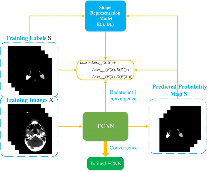
The flowchart of the training process of FCNN. [Color figure can be viewed at wileyonlinelibrary.com]

2.D. Data acquisition and pre‐processing

The dataset used for the training and evaluation of the proposed framework was obtained from Public Domain Database for Computational Anatomy (PDDCA) version 1.4.1. The original CT data were derived from the Radiation Therapy Oncology Group (RTOG) 0522 study, a multi‐institutional clinical trial led by Kian Ang.³² The dataset contains 48 patient CT volumes with anisotropic pixel spacing ranging from 0.76 to 1.27 mm and inter‐slice thickness ranging from 1.25 to 3.0 mm. It is worth pointing out that the same dataset was used in MICCAI 2015 Head and Neck Auto Segmentation Grand Challenge. The result of the competition was summarized in Ref. 4. Thirty‐two of the 48 patients in the database with complete manual labeling of nine structures, including left and right parotid glands, brainstem, optic chiasm, optic nerves (both left and right), mandible, and submandibular glands (both left and right), were used in this study. The remaining 16 patients missed one or more of the nine structures and were excluded.

The 32 patients were randomly and asymmetrically divided into a training set (22 subjects) and a testing test (10 subjects). To homogenize the data, reduce memory consumption, and increase computational speed, all images were re‐sampled to isotropic resolution of 2 × 2 × 2 mm³ and then cropped to fit the patient contour, resulting in a uniform matrix size of 144 × 144 × 112, which was used for both training and testing.

To tackle the model robustness and avoid overfitting, we augmented the data by introducing rotation (90°, 180°, 270°) and randomly scaling between 0.8 and 1.2. In total, we used 102 variations to train our FCNN and SRM.

2.E. Evaluation metrics

Five metrics including Dice Similarity Coefficient (DSC), Positive Predictive Value (PPV), Sensitivity (SEN), Average Surface Distance (ASD), and 95% maximum surface distance (95% SD) are used to quantitatively evaluate the performance of the proposed segmentation framework against manual segmentation. The segmentation evaluation metrics are defined as below:

• Dice Similarity Coefficient (DSC) measures the volumetric overlap degree between the manual and automatic segmentations. It is defined as³³:

  $$DSC=\frac{2\Vert A\cap B\Vert }{\Vert A\Vert +\Vert B\Vert }$$ (3)

where A and $B$ refer to the set of nonzero voxels in the manual and automatic segmentations, respectively.

• Positive Predictive Value (PPV) measures the proportion of correctly nonzero voxels in the automatically segmented organ. It is defined as:

  $$PPV=\frac{\Vert A\cap B\Vert }{\Vert B\Vert }$$ (4)

• Sensitivity (SEN) measures the proportion of correctly nonzero voxels in the manually segmented organ. It is defined as:

  $$SEN=\frac{\Vert A\cap B\Vert }{\Vert A\Vert }$$ (5)

• Average Surface Distance (ASD) measures the average distance between the surface of A and B. It is defined as³⁴:

  $$ASD=\frac{1}{2}\left\{\frac{{\sum }_{z\in B}d(z,A)}{|B|}+\frac{{\sum }_{u\in A}d(u,B)}{|A|}\right\}$$ (6)

  where d(z, A) is the minimum distance of voxel z on the automatically segmented organ surface B to the voxels on the ground truth surface A, d(u, B) is the minimum distance of voxel u on the ground truth surface A to the voxels on the automatically segmented organ surface B.

• 95% Maximum Surface Distance (95% SD) is based on the calculation of 95th percentile of the distances between the boundary points of A and B, which is expected to eliminate the impact of a very small subset of incurrent segmentations on the evaluation of the overall segmentation quality.

The paired Student's t‐test is used to compare the segmentation accuracy of FCNN with and without SRM. Results are considered significant if P < 0.05.

2.F. Implementation details

Our experiments were carried out using Keras³⁵ with Tensorflow, whose backend is Python 2.7. The hardware is a GeForce GTX 1080 GPU for acceleration. The learning rate was initially set as 5 × 10⁻⁴, which was divided by a factor of 5 every 10 epochs when the validation loss stopped improving. The weights of the shape representation loss term λ ₁ and reconstruction loss term λ ₂ in the loss function were set as 0.01 and 0.001, respectively. All the networks were optimized using the Adam algorithm.³⁶ Moreover, to prevent over‐fitting, a dropout value of 0.3 and an early stopping strategy were utilized in this work if there was no improvement in the validation loss after 50 epochs.

It took approximately 2 and 10 h to train the SRM and FCNN, respectively. With the trained network, the average time for segmenting all nine OARs in a testing H&N CT volume was 9.50 s, which was a significant improvement over conventional segmentation methods.

3. Results

3.A. Qualitative evaluation

Figures 4, 5, 6, 7 visually compare the segmentation results of the 9 H&N OARs between the proposed method with and without the SRM. It can be observed that although FCNN alone can approximately segment the OARs, it leads to isolated false‐positive volumes as shown in the first rows of Figs. 4 and 5. The additional SRM regularization removes these false‐positive islands by better regularizing the segmentation shapes (Fig. 4 subject 1). Leveraging the latent shape representation learned by SRM, the FCNN segmentation results show robustness to inter‐patient shape variations.

Figure 4.

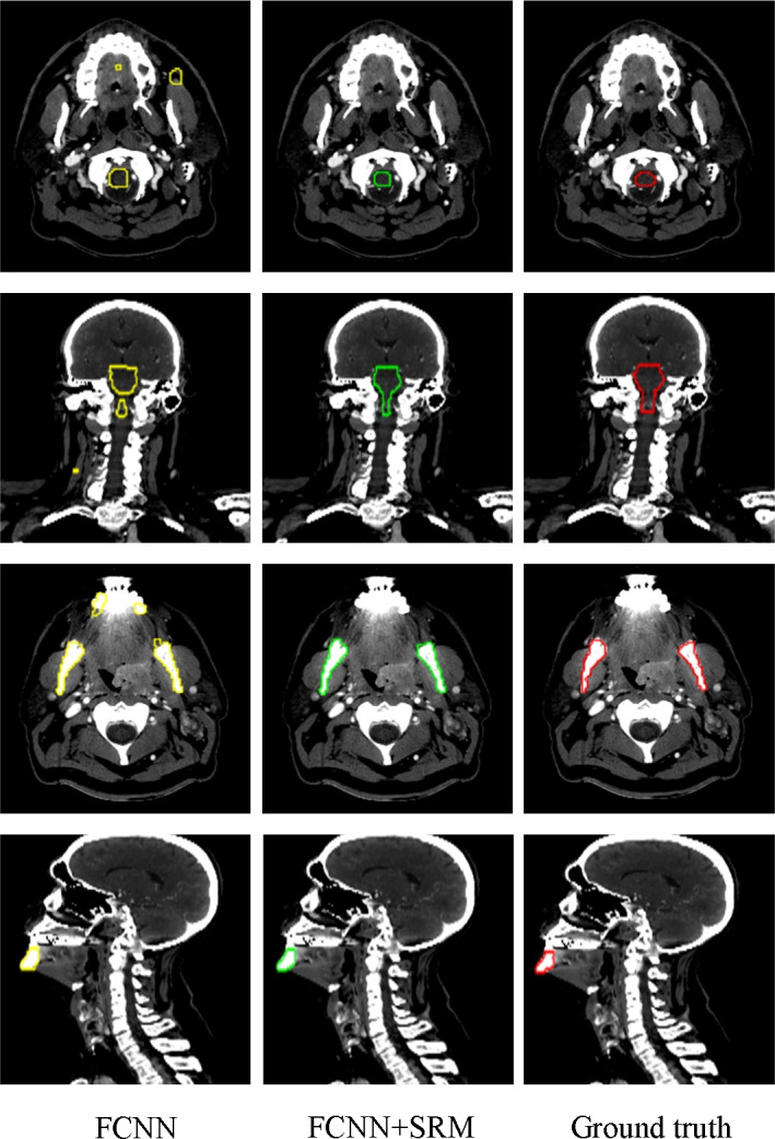
Visual comparison of segmentation results of the brainstem (the first and second rows) and mandible (the third and fourth rows) using our method with and without SRM. The three columns show the segmentation results and ground truth overlaid on the CT. Yellow and green denote the FCNN segmentations with and without SRM respectively. The red contours denote the ground truth. [Color figure can be viewed at wileyonlinelibrary.com]

Figure 5.

Visual comparison of segmentation results of the parotid glands (the first and second rows) and submandibular glands (the third and fourth rows) using our method with and without SRM. The three columns show the segmentation results and ground truth overlaid on the CT. Yellow and green denote the FCNN segmentations with and without SRM respectively. The red contours denote the ground truth. [Color figure can be viewed at wileyonlinelibrary.com]

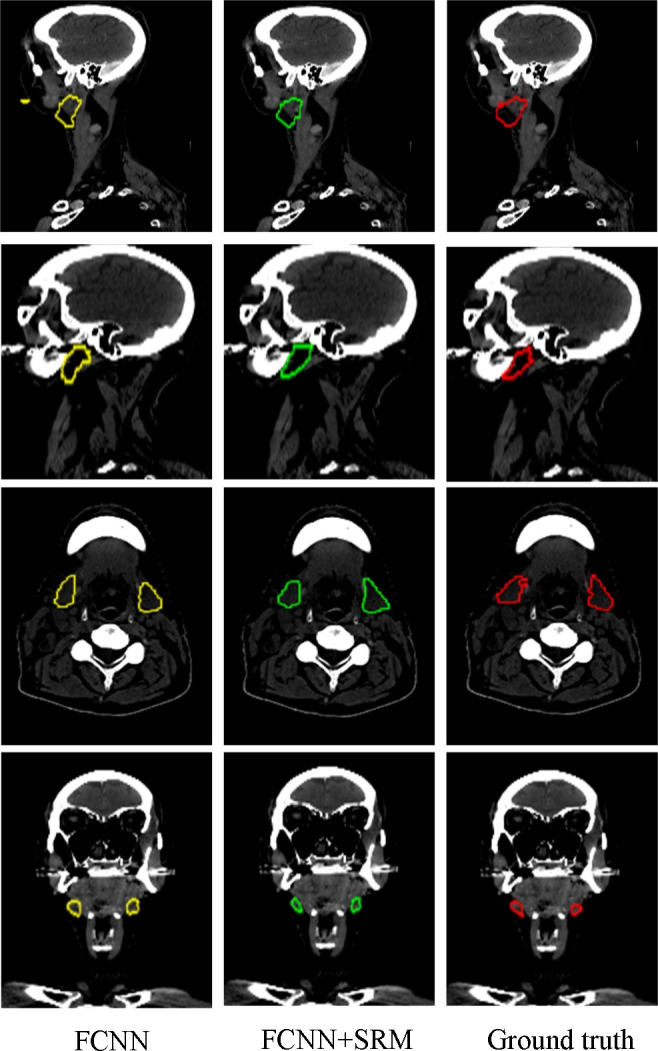
Figure 6.

Visual comparison of segmentation results of the optic chiasm (the first and second rows) and optic nerves (the third row) using our method with and without SRM. The three columns show the segmentation results and ground truth overlaid on the CT. Yellow and green denote the FCNN segmentations with and without SRM respectively. The red contours denote the ground truth. [Color figure can be viewed at wileyonlinelibrary.com]

Figure 7.

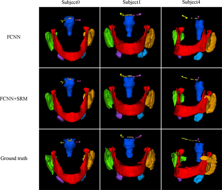
3D visual representation of H&N OARs segmented by the proposed method. The first and second rows present the segmentations using our method with and without SRM; the third row shows the ground truth. Brainstem (Dark blue), Optic Chiasm (Brown), Mandible (Red), Left Optic Nerve (pink), Right Optic Nerve (Yellow), Left parotid gland (Orange), Right Parotid gland (green), Left Submandibular (Light blue), Right Submandibular (Purple). [Color figure can be viewed at wileyonlinelibrary.com]

3.B. Quantitative evaluation

Table 1 shows the average Dice Similarity Coefficient, Positive Predictive Value (PPV), Sensitivity (SEN), Average Surface Distance (ASD), 95% Maximum Surface Distance (95%SD), and the standard deviation of all the OARs by FCNN with and without SRM. Figure 8 shows the bar plots of DSC (%) for all organs compared to FCNN alone and CNN.²⁴ It can be observed that our method leads to a significant improvement in segmentation accuracy for all considered organs by incorporating the shape constraint provided by SRM. The paired Student's t‐test further demonstrates that the segmentation performance of FCNN with SRM is significantly higher than that of FCNN alone (P = 0.0018). Meanwhile, as illustrated in Fig. 8, the standard deviations of our method are smaller than those of the other method, demonstrating superior robustness to inter‐patient variability.

Table 1.

Quantitative comparison of segmentation results between our method with and without SRM

Organ	Method	DSC (%)	PPV (%)	SEN (%)	ASD (mm)	95%SD (mm)
Brainstem	FCNN	82.86 ± 2.68	81.72 ± 4.75	84.06 ± 4.54	1.58 ± 0.33	4.05 ± 1.09
	FCNN+SRM	86.97 ± 2.95	85.39 ± 2.15	87.99 ± 2.57	1.17 ± 0.56	4.01 ± 0.93
Optic chiasm	FCNN	46.19 ± 8.35	40.91 ± 12.62	51.63 ± 6.68	1.35 ± 0.98	3.76 ± 3.05
	FCNN+SRM	58.35 ± 10.28	55.92 ± 10.03	60.95 ± 9.85	0.65 ± 0.21	2.17 ± 1.04
Mandible	FCNN	92.07 ± 1.15	94.65 ± 1.34	91.09 ± 1.77	0.51 ± 0.12	2.01 ± 0.83
	FCNN+SRM	93.60 ± 1.21	94.86 ± 4.52	92.09 ± 2.26	0.37 ± 0.11	1.50 ± 0.32
Left optic nerve	FCNN	60.66 ± 9.01	59.67 ± 7.50	61.62 ± 4.09	1.94 ± 0.38	2.65 ± 1.08
	FCNN+SRM	65.31 ± 5.75	63.74 ± 5.77	67.11 ± 4.20	1.14 ± 0.75	2.52 ± 1.04
Right optic nerve	FCNN	61.94 ± 4.63	54.00 ± 7.5	68.97 ± 9.38	1.33 ± 0.59	3.29 ± 1.23
	FCNN+SRM	68.89 ± 4.71	60.73 ± 5.77	74.00 ± 5.54	1.15 ± 0.65	2.90 ± 1.88
Left parotid	FCNN	81.69 ± 3.23	84.93 ± 1.35	77.26 ± 4.85	2.28 ± 1.78	5.35 ± 3.30
	FCNN+SRM	83.87 ± 2.87	86.48 ± 1.52	80.07 ± 5.30	0.96 ± 0.34	3.97 ± 2.15
Right parotid	FCNN	81.31 ± 5.88	81.91 ± 1.35	81.06 ± 7.73	1.68 ± 0.67	4.83 ± 2.95
	FCNN+SRM	83.46 ± 2.34	84.11 ± 1.52	82.42 ± 4.55	1.12 ± 0.56	4.20 ± 1.27
Left submandibular	FCNN	71.55 ± 5.51	76.02 ± 4.94	67.57 ± 6.12	2.21 ± 1.28	5.98 ± 2.14
	FCNN+SRM	76.7 ± 7.31	80.20 ± 8.10	72.28 ± 6.35	0.90 ± 0.46	5.59 ± 3.93
Right submandibular	FCNN	75.48 ± 6.49	76.49 ± 6.01	73.83 ± 7.43	1.66 ± 0.42	5.47 ± 2.42
	FCNN+SRM	81.31 ± 6.45	77.45 ± 6.43	85.35 ± 6.09	1.33 ± 0.57	4.84 ± 1.67

Figure 8.

Bar chart results of CNN, and FCNN with and without SRM. Colored bars represent the average DSC(%) value of segmentation results of each structure by CNN,²³ and using our proposed method with and without SRM. Note that the brainstem was not segmented in Ref. [23]. [Color figure can be viewed at wileyonlinelibrary.com]

3.C. Comparison with state‐of‐the‐art methods

The FCNN+SRM segmentation method is compared with several state‐of‐the‐art methods based on DSC (%) in Table 2. Table 3 compares the segmentation time to segment a new patient using our method versus the state‐of‐the‐art methods. It is worth noting that the active appearance model‐based method³⁶ was the winner of the MICCAI Grand Challenge using the same dataset, providing a frame of reference for direct comparison. FCNN+SRM shows competitive performance in direct comparison with the active appearance model method, and in indirect comparison with the atlas and CNN methods using different patient data. Furthermore, the segmentation time is shorter than that previously reported.

Table 2.

Comparison of segmentation accuracy between the state‐of‐the‐art methods and our method (Dice %), bold fonts indicate the best performer for that structure

Organ/method	Atlas‐based5	Model‐based37	CNN24	FCNN(our)	FCNN+SRM(our)
Brainstem	82	87 ± 4	Unavailable	82.86 ± 2.68	86.97 ± 2.95
Chiasm	Unavailable	35 ± 16	37.4 ± 13.4	46.19 ± 8.35	58.35 ± 10.28
Mandible	89	91 ± 2	89.5 ± 3.6	92.07 ± 1.15	93.67 ± 1.21
Left optic nerve	Unavailable	63 ± 5	63.9 ± 6.9	60.66 ± 9.01	65.31 ± 5.75
Right optic nerve	Unavailable	63 ± 5	64.5 ± 7.5	61.94 ± 4.63	68.89 ± 4.74
Left parotid	82	82 ± 10	76.6 ± 6.1	81.69 ± 3.23	83.49 ± 2.29
Right parotid	82	82 ± 10	77.9 ± 5.4	81.31 ± 5.88	83.18 ± 1.45
Left Submandibular	69	78 ± 8	69.7 ± 13.3	71.55 ± 5.51	75.48 ± 6.49
Right submandibular	69	78 ± 8	73.0 ± 9.2	76.7 ± 7.31	81.31 ± 6.45

Table 3.

Comparison of segmentation time between the state‐of‐the‐art methods and our method

Method	Segmentation time	Experimental equipment
Atlas‐based5 (multi‐atlas)	Over an hour per patient for 9 H&N organs	CPU
Model‐based37	30 min per image for 9 H&N organs	CPU
CNN24	4 min per patient for 13 H&N organs	GPU
Our	9.50 s per patient for 9 H&N organs	GPU

4. Discussion

In this work, we present a robust and efficient segmentation method for H&N CT images that combines the strengths of existing methods. The proposed method uses a novel shape representation model (ie, SRM), to learn the highly representative shape characteristics of H&N OARs, model the relationships among them, constrain the training of the segmentation network (ie, FCNN), and improve its segmentation performance. During the training of FCNN, SRM serves as a regularizer to reduce false‐positivity and help the final segmentation of FCNN to better follow the shape distributions of the H&N OARs.

A direct comparison between FCNN with and without SRM demonstrates that SRM significantly improves segmentation accuracy for nine organs with varying sizes, morphological complexities, and CT contrasts.

Although the performance of compared methods can be influenced by underlying H&N datasets, the SRM+FCNN method is shown to be competitive when compared with existing conventional segmentation methods and a deep‐learning based method by demonstrating consistently higher DSC (%) and lower standard deviations. Another advantage of our method is that post‐processing was not needed to produce the completive results, thus further improving its generalizability.

Besides SRM regularization, we made several additional improvements to the existing deep learning segmentation studies. In the current implementations, owing to the difficulties of optimizing 3D networks and inadequate training samples, many existing deep learning segmentation studies formulated the problem as a patch‐wise classification task, which is inefficient due to computational redundancy and restricted to learning local features that are only visible in individual patches.²⁵ In this paper, we employ a fully convolutional architecture where all layers are either convolutional or pooling. As a result, the network can use arbitrarily sized volumetric images as input, and then perform probability predictions. This novel architecture simultaneously eliminates computational redundancy and enables learning global features of the images. To further improve the convergence rate, a deep supervision mechanism²⁵ is integrated into our FCNN by providing additional guidance to the training of the lower layers in the network.

Besides segmentation performance, the improvements in algorithm resulted in a major advantage in computational speed. The incorporation of SRM slightly increases the computational cost in the training stage of FCNN. After training, multiple OARs in a new patient CT can be segmented in under 10 s using FCNN. The fast segmentation time is particularly valuable to applications such as adaptive radiotherapy.

The performance of the novel segmentation network can be limited by latent anatomy shape characteristics captured by the SRM. In the case where the testing patient has substantially different anatomies, such as the post‐surgical patients, an incorrect SRM may reduce segmentation network performance. In such case, the SRM regularization may require a more specific training dataset. Furthermore, as a regularization term, the severity of the problem is expected to be less than that of the atlas and statistical shape methods which rely on the shape representation model alone. There are two more limitations of this study. First, among the three existing methods used for comparison, only one was performed on the same dataset. This difference prevents us from more clearly affirming the accuracy of our method. Second, the training and testing datasets were limited in size. Although good performance was observed, its robustness and potential improvement need to be tested on a larger patient dataset and preferably in a multi‐institutional study.

5. Conclusion

A fully automatic and efficient multi organ segmentation method for H&N CT images is demonstrated and tested. When combined with SRM, FCNN is constrained to follow the latent shape characteristics of OARs in the training set, which not only improves the segmentation accuracy of FCNN, but also eliminates the need for post‐processing. The SRM‐constrained FCNN shows competitive performance compared to conventional atlas and statistical shape‐based methods as well as a deep learning method, in both accuracy and computational efficiency.

References

- 1. Chaturvedi AK, Anderson WF, Lortet‐tieulent J, et al. Worldwide trends in incidence rates for oral cavity and oropharyngeal cancers. J Clin Oncol. 2013;31:4550–4559. [DOI] [PMC free article] [PubMed] [Google Scholar]
- 2. Wang XS, Eisbruch A. IMRT for head and neck cancer: reducing xerostomia and dysphagia. J Radiat Res. 2016;57:i69–i75. [DOI] [PMC free article] [PubMed] [Google Scholar]
- 3. Breunig J, Hernandez S, Lin J, et al. A system for continual quality improvement of normal tissue delineation for radiation therapy treatment planning. Int J Radiat Oncol Biol Phys. 2012;83:e703–e708. [DOI] [PubMed] [Google Scholar]
- 4. Raudaschl PF, Zaffino P, Sharp GC, et al. Evaluation of segmentation methods on head and neck CT: auto‐segmentation challenge 2015. Med Phys. 2017;44:2020–2036. [DOI] [PubMed] [Google Scholar]
- 5. Han X, Hoogeman MS, Levendag PC, et al. Atlas‐based auto‐segmentation of head and neck CT images. In: MICCAI Proceedings; 2008:434–441. [DOI] [PubMed]
- 6. Urban S, Tanacs A. Atlas‐based global and local RF segmentation of head and neck organs on multimodal MRI images. In: ISPA Proceedings; 2017:99–103.
- 7. Zhao T, Ruan D. Learning image based surrogate relevance criterion for atlas selection in segmentation. Phys Med Biol. 2016;61:4223–4234. [DOI] [PubMed] [Google Scholar]
- 8. Cootes TF, Edwards GJ, Taylor CJ. Active appearance models. IEEE Trans Pattern Anal Mach Intell. 2001;23:681–685. [Google Scholar]
- 9. Cootes TF, Taylor CJ, Cooper DH, Graham J. Active shape models‐their training and application. Comput Vis Image Underst. 1995;61:38–59. [Google Scholar]
- 10. Fritscher KD, Peroni M, Zaffino P, Spadea MF, Schubert R, Sharp G. Automatic segmentation of head and neck CT images for radiotherapy treatment planning using multiple atlases, statistical appearance models, and geodesic contours. Med Phys. 2014;41:1–11. [DOI] [PMC free article] [PubMed] [Google Scholar]
- 11. Fortunati V, Verhaart RF, Van Der Lijn F, et al. Hyperthermia critical tissues automatic segmentation of head and neck CT images using atlas registration and graph cuts. In: ISBI Proceedings; 2012:1683–1686.
- 12. Arindra A, Setio A, Ciompi F, et al. Pulmonary nodule detection in CT images: false positive reduction using multi‐view convolutional networks. IEEE Trans Med Imaging. 2016;35:1160–1169. [DOI] [PubMed] [Google Scholar]
- 13. Kawahara J, BenTaieb A, Hamarneh G. Deep features to classify skin lesions. In: ISBI Proceedings; 2016:1397–1400.
- 14. de Vos BD, Wolterink JM, deJong PA , Viergever MA, Išgum I. 2D image classification for 3D anatomy localization: employing deep convolutional neural networks. In: SPIE Proceedings. 2016:97841Y.
- 15. Hwang S, Kim HE. Self‐Transfer Learning for Fully Weakly Supervised Object Localization. arXiv preprint arXiv:1602.01625; 2016.
- 16. Andernatt S, Pezold S, Cattin P. Multi‐dimensional gated recurrent units for the segmentation of biomedical 3D‐data. In: DLMIA Proceedings. 2016:142‐151.
- 17. Brosch T, Tang LYW, Yoo Y, Li DKB, Traboulsee A, Tam R. Deep 3D convolutional encoder networks with shortcuts for multiscale feature integration applied to multiple sclerosis lesion segmentation. IEEE Trans Med Imaging. 2016;35:1229–1239. [DOI] [PubMed] [Google Scholar]
- 18. Simonovsky M, Gutiérrez‐Becker B, Mateus D, et al. A deep metric for multimodal registration. In: MICCAI Proceedings; 2016:10‐18.
- 19. Shah A, Conjeti S, Navab N, Katouzian A. Deeply learnt hashing forests for content based image retrieval in prostate MR images. In: SPIE Proceedings; 2016:978414.
- 20. Oktay O, Bai W, Lee W, et al. Multi‐input cardiac image super‐resolution using convolutional neural networks. In: MICCAI Proceedings; 2015:1275‐1283.
- 21. Kamnitsas K, Ledig C, Newcombe VFJ, et al. Efficient multi‐scale 3D CNN with fully connected CRF for accurate brain lesion segmentation. Med Image Anal. 2017;36:61–78. [DOI] [PubMed] [Google Scholar]
- 22. Moeskops P, Viergever MA, Mendrik AM, De Vries LS, Benders MJNL, Isgum I. Automatic segmentation of MR brain images with a convolutional neural network. IEEE Trans Med Imaging. 2016;35:1252–1261. [DOI] [PubMed] [Google Scholar]
- 23. Havaei M, Davy A, Warde‐Farley D, et al. Brain tumor segmentation with deep neural networks. Med Image Anal. 2017;35:18–31. [DOI] [PubMed] [Google Scholar]
- 24. Ibragimov B, Xing L. Segmentation of organs‐at‐risks in head and neck CT images using convolutional neural networks. Med Phys. 2017;44:547–557. [DOI] [PMC free article] [PubMed] [Google Scholar]
- 25. Kayalibay B, Jensen G, van der Smagt P. CNN‐based Segmentation of Medical Imaging Data. arXiv preprint arXiv:1701.03056 2017.
- 26. Wang Z, Wei L, Wang L, Gao Y, Chen W, Shen D. Hierarchical vertex regression‐based segmentation of head and neck ct images for radiotherapy planning. IEEE Trans Image Process. 2018;27:923–937. [DOI] [PMC free article] [PubMed] [Google Scholar]
- 27. Ravishankar H, Venkataramani RB, Thiruvenkadam S, Sudhakar P. Learning and Incorporating Shape Models for Semantic Segmentation. In: MICCAI Proceedings; 2017:203–211.
- 28. Lu D, Popuri K, Ding GW, Balachandar R, Beg MF. Multiscale deep neural network based analysis of FDG‐PET images for the early diagnosis of Alzheimer's disease. Med Image Anal. 2018;46:26–34. [DOI] [PubMed] [Google Scholar]
- 29. Dou Q, Yu L, Chen H, et al. 3D deeply supervised network for automated segmentation of volumetric medical images. Med Image Anal. 2017;41:40–54. [DOI] [PubMed] [Google Scholar]
- 30. Ronneberger O, Fischer P, Brox T. U‐net: Convolutional nerworks for biomedical image segmentation. In: MICCAI Proceedings; 2015:234–241.
- 31. Glorot X, Bengio Y. Understanding the difficulty of training deep feedforward neural networks. In: AISTATS Proceedings; 2010:249‐256.
- 32. Ang KK, Zhang Q, Rosenthal DI, et al. Randomized phase III trial of concurrent accelerated radiation plus cisplatin with or without cetuximab for stage III to IV head and neck carcinoma: RTOG 0522. J Clin Oncol. 2014;32:2940–2950. [DOI] [PMC free article] [PubMed] [Google Scholar]
- 33. Dice LR. Measures of the amount of ecologic association between species. Ecology. 2009;26:297–302. http://www.jstor.org/stable/1932409. [Google Scholar]
- 34. Kitware . Contour mean distance image filter. Available: http://www.itk.org/Doxygen/html/classitk_1_1ContourMeanDistanceImageFilter.html; 2015.
- 35. Chollet F. Keras. https://github.com/fchollet/Keras; 2015.
- 36. Kingma DP, Ba J. Adam: A Method for Stochastic Optimization. In: ICLR Proceedings; 2015:1–41.
- 37. Mannion‐Haworth R, Bowes M, Ashman A, Guillard G, Brett A, Vincent G. Fully Automatic Segmentation of Head and Neck Organs Using Active Appearance Models. In: Presented in Head and Neck Auto‐Segmentation Challenge 2015. Available: http://www.midasjournal.org/browse/publication/965; 2016.