APPLE picker: Automatic particle picking, a low-effort cryo-EM framework

Abstract

Particle picking is a crucial first step in the computational pipeline of single-particle cryo-electron microscopy (cryo-EM). Selecting particles from the micrographs is difficult especially for small particles with low contrast. As high-resolution reconstruction typically requires hundreds of thousands of particles, manually picking that many particles is often too time-consuming. While template-based particle picking is currently a popular approach, it may suffer from introducing manual bias into the selection process. In addition, this approach is still somewhat time-consuming. This paper presents the APPLE (Automatic Particle Picking with Low user Effort) picker, a simple and novel approach for fast, accurate, and template-free particle picking. This approach is evaluated on publicly available datasets containing micrographs of β-galactosidase, T20S proteasome, 70S ribosome and keyhole limpet hemocyanin projections.

1. Introduction

Single-particle cryo-electron microscopy (cryo-EM) aims to determine the structure of 3D specimens (macromolecules) from multiple 2D projections. In order to acquire these 2D projections, a solution containing the macromolecules is frozen in vitreous ice on either carbon or gold film, thus creating a sample grid. An electron beam then passes through the ice and the macromolecules frozen within, creating 2D projections.

Unfortunately, due to radiation damage only a small number of imaging electrons can be used in the creation of the micrograph. As a result, micrographs have a low signal-to-noise ratio (SNR). An elaboration on the noise model can be found in (Sigworth, 2004).

Since micrographs typically have low SNR, each micrograph consists of regions of noise and regions of noisy 2D projections of the macromolecule. In addition to these, micrographs also contain regions of non-significant information stemming from contaminants such as carbon film.

Different types of regions have different typical intensity values. The intensity values of the micrograph are determined by the number of electrons that have passed through the sample grid, and are influenced by the microscope’s contrast transfer function. Due to these factors, regions of the micrograph that contain only noise will typically have higher intensity values than other regions. In addition, regions containing a particle typically have higher variance than regions containing noise alone (Nicholson and Glaeser, 2001; van Heel, 1982). Thus, two cues that can be used for projection image identification are the mean and variance of the image.

In order to determine the 3D structure at high resolution, many projection images are needed, often in the hundreds of thousands. Thus, the first step towards 3D reconstruction of macromolecules consists of determining regions of the micrograph that contain a particle as opposed to regions that contain noise or contaminants. This is the particle picking step.

A fully manual selection of hundreds of thousands of 2D projections is tedious and time-consuming. For this reason, semi-automatic and automatic particle picking is a much researched problem for which numerous frameworks have been suggested. Solutions to the particle picking problem include edge detection (Harauz and Fong-Lochovsky, 1989), deep learning (Ogura and Sato, 2004; Wang et al., 2016; Zhu et al., 2016), support vector machine classifiers (Aebeláez et al., 2011), and template matching (Frank and Wagenknecht, 1983).

Template matching is a popular approach to particle picking. The input to template matching schemes consists of a micrograph and images containing 2D templates to match. These templates can be, for example, generated from manually selected particle projections. The aim is to output the regions in the micrograph that contain the sought-after templates.

The basic idea behind this approach (Chen and Grigorieff, 2007; Frank and Wagenknecht, 1983; Langlois et al., 2014; Ludtke et al., 1999; Scheres, 2015) is that the cross-correlation¹ between a template image and a micrograph is larger in the presence of the template. An issue with this method is the high rate of false detection. This issue stems from the fact that given enough random data, meaningless noise can be perceived as a pattern. This problem was exemplified in (Henderson, 2013; Shatsky et al., 2009), where an image of Einstein was used as the template and matched to random noise. Even though the image was not present in the noise images, a reconstruction from the best-matched images yielded the original Einstein image.

One example of a template-based framework is provided in RELION (Scheres, 2015; Scheres, 2012; Scheres, 2012). In this framework, the user manually selects approximately one thousand particles from a small number of micrographs. These particle images are then 2D classified to generate a smaller number of template images that are used to automatically select particles from all micrographs. These particle images are then classified in order to identify non-particles. Additional examples of template-based frameworks include SIGNATURE (Chen and Grigorieff, 2007) which employs a post-processing step that ensures the locations of any two picked particles cannot overlap, and gEMpicker (Hoang et al., 2013) which employs several strategies to speed up template matching.

Template matching can also be performed without the input of template images. One example of this is the DoG picker (Voss et al., 2009), which is based on difference of Gaussians and is suitable for identifying blobs of a certain size in the micrograph. Another templatefree particle picking framework is gautomatch (Zhang, 2017). In addition, RELION allows the use of a Gaussian blob as a template.

In this paper we propose a particle picking framework that is data-adaptive in the sense that no manual selection is used and no templates are involved. Instead, the APPLE picker uses a set of automatically selected reference windows to detect the existence of a particle projection. This set includes both particle and noise windows. We show that it is possible to determine the presence of a particle in any query image (i.e., region of the micrograph) through cross-correlation with each window of the reference set. Specifically, in the case where the query image contains noise alone, since there is no template to match, the cross-correlation coefficients should not indicate the presence of a template regardless of the actual content of each reference window. On the other hand, in the case where the query image contains a particle, the coefficients will depend on the content of each reference window.

Our cross-correlation based procedure can provide a determination of content for each window in the micrograph. However, in the interest of reducing runtime, we select a subset of windows as our query images. Once their content is determined, the query images most likely to contain a particle and those most likely to contain noise can be used to train a classifier. The output of this classifier is used for particle picking.

We note that our formulation can ignore the contrast transfer function (CTF). This is because the CTF is roughly the same throughout the micrograph and our particle selection procedure performs on the individual micrograph level. Thus, while CTF-correction is not strictly necessary, we discuss the advantage of applying our framework to CTF-corrected micrographs in Section 2.6.

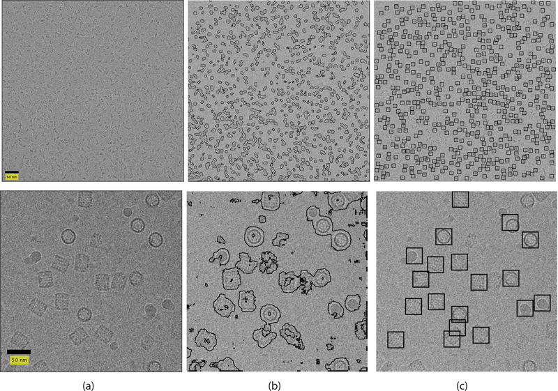
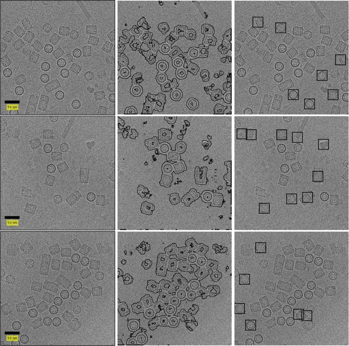
We test our framework on publicly available datasets of β-galactosidase (Chen et al., 2013; Scheres, 2015; Scheres and Chen, 2012), T20S proteasome (Danev and Baumeister, 2016), 70S ribosome (Fischer et al., 2016) and keyhole limpet hemocyanin (Zhu et al., 2003; Zhu et al., 2004). Some sample results are presented in Fig. 1. Code for our framework is publicly available.²

Fig. 1.

Result of our suggested framework. The left column contains micrographs. The middle column contains the output of the classifier. The right column contains the picked particles. Top row contains a β-galactosidase micrograph. Bottom row contains a KLH micrograph.

2. Material and methods

In Section 2.1 we detail our method for determining the content of a single query image g ∈ ℝ^n×n, where the query image is a window extracted from the micrograph and n is chosen such that the window size is slightly smaller than the particle size (which we assume is known).³This method necessitates the use of a reference set ${\left\{f_m\in {\mathbf{ℝ}}^{n\times n}\right\}}_{m=1}^B$ selected from the micrograph in the automatic manner detailed in Section 2.2. We generalize our method to particle picking from the full micrograph in Section 2.3. Section 2.4 improves localization through the use of a fast classification step. The complete method, known as the APPLE picker, is described in Section 2.5. We discuss the advantage of CTF correction in Section 2.6.

2.1. Determining the content of a query image

The idea behind traditional template matching methods is that the cross-correlation score of two similar images is high. Specifically, a template image known to contain a particle can be used in order to identify similar patterns in the micrograph using cross-correlation. In this section we show that the same idea can be used to determine the content of regions of the micrograph even when no templates are available. To this end we use the cross-correlation between a query image g and a set of reference images ${\left\{f_m\right\}}_{m=1}^B$. The cross-correlation function is (Nicholson and Glaeser, 2001)

$$c_{f_m,g}(x,y)={\displaystyle \sum _{x^{\prime }}{\displaystyle \sum _{y^{\prime }}{f}_m}}\left(x^{\prime },y^{\prime }\right)g\left(x+x^{\prime },y+y^{\prime }\right).$$ (1)

This function can be thought of as a score associated with f_m, g and an offset (x y, ).

The cross-correlation score at a certain offset does not in itself have much meaning without the context of the score in nearby offsets. For this reason we define the following normalization on the cross-correlation function

$${\widehat{c}}_{f_m,g}(x,y)=c_{f_m,g}(x,y)-\frac{1}{n^2}{\displaystyle \sum _{x^{\prime }}{\displaystyle \sum _{y^{\prime }}{c}_{f_m,g}}}\left(x^{\prime },y^{\prime }\right),$$ (2)

where the second term is the mean of $c_{f_m,g}\in {\mathbf{ℝ}}^{n\times n}$. We call (2) a normalization since it shifts all cross-correlations to a common baseline.

Consider the case where query image g contains a particle. The score $c_{f_m,g}(x,y)$ is expected to be maximized when f_m contains a particle with a similar view. In this case there will be some offset (x, y) such that the images f_m and g match best, and $c_{f_m,g}(x,y)>c_{f_m,g}\left(x^{\prime },y^{\prime }\right)$ for all other offsets (x′, y′). Thus,

$$c_{f_m,g}(x,y)>\frac{1}{n^2}{\displaystyle \sum _{x^{\prime }}{\displaystyle \sum _{y^{\prime }}{c}_{f_m,g}}}\left(x^{\prime },y^{\prime }\right).$$ (3)

In other words, ${\widehat{c}}_{f_m,g}(x,y)$ is expected to be large and positive. In this case, we say g has a strong response to f_m.

Next, consider the case where query image g contains no particle. In this case there should not exist any offset (x, y) that greatly increases the match for any f_m. Thus typically ${\widehat{c}}_{f_m,g}(x,y)$ is comparatively small in magnitude. In other words, g has a weak response to f_m.

We define a response signal s_g such that

$${\mathbf{s}}_g(m)=\underset{x,y}{\max }{\widehat{c}}_{f_m,g}(x,y),m=1,\dots ,B.$$ (4)

This signal is associated with a single query image g. Each entry s_g(m) contains the maximal normalized cross-correlation with a single reference image f_m. Thus, the response signal captures the strength of the response of the query image to each of the reference images.

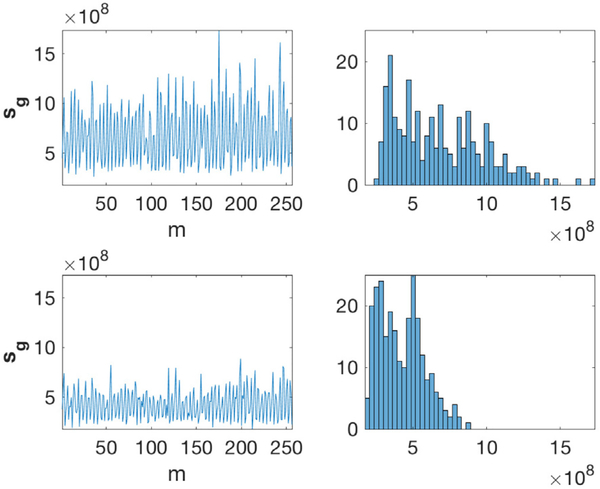
We suggest that s_g can be used to determine the content of g. If the query image contains a particle, s_g will show a high response to reference images containing a particle with similar view and a comparatively low response to other images. As a consequence, s_g will have several high peaks. On the other hand, if the query image contains noise alone, s_g will have relatively uniform content. This idea is shown in Fig. 2.

Fig. 2.

Response signal (s_g) vs index of reference window (m) of a particle image (top) and a noise image (bottom). The left column contains the response signals (see (4)). The right column contains histograms of the response signals.

The above is true despite the high rate of false positives in cross-correlation-based methods. This is due to the comparison of each query image to multiple reference windows. The redundancy causes robustness to false positives.

2.2. Reference set selection

The set of reference images ${\left\{f_m\right\}}_{m=1}^B$ could contain all possible windows in the micrograph. However, this would lead to unnecessarily long runtimes. Thus, we suggest to choose a subset of B windows from the micrograph, where each of these windows is either likely to contain a particle or likely to contain noise alone.

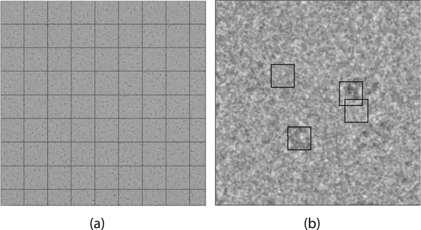
In order to automatically select this subset, we first divide the micrograph into B/4 non-overlapping containers. A container is some rectangular portion of the micrograph. Each container holds many n × n windows. Fig. 3a is an example of the division of a micrograph into containers.

Fig. 3.

(a) Containers of a micrograph of the β-galactosidase dataset. (b) Single container with four windows of interest.

As mentioned in Section 1 (fourth paragraph), regions containing noisy projections of particles typically have lower intensity values and higher variance than regions containing noise alone. Thus we find that the window with the lowest mean intensity in each container likely contains a particle and the window with the highest mean intensity likely does not. We extract these windows from each container and include them in the reference set. We do this also for the windows that have the highest and lowest variance in each container. This procedure provides a set of B reference windows. Fig. 3b presents the reference windows extracted from a single container. We suggest setting B to approximately 300.

The set of reference windows must contain both windows with noise and windows with particles. It may seem counter-intuitive to include noise windows in a reference set. However, for roughly symmetric particles (i.e., particles with similar projections from each angle), any query image will have a similar response to every reference image which contains a particle. Thus, if noise images were not included in the reference set, the response signal s_g would be uniform regardless of the content of g.

2.3. Generalization to micrographs

We extract a set of M query images from the micrograph. These images should have some overlap. In addition, their union should cover the entire micrograph. For example, we can choose windows on a grid with step size n/2. In order to determine the content of each query image g, we examine the number of entries that are over a certain threshold, i.e.,

$$k\left({\mathbf{s}}_g\right)=\left|\left\{i\text{such}\text{that}{\mathbf{s}}_g(i)>t\right\}\right|,$$ (5)

where the threshold t is determined according to the set of response signals and is experimentally set to

$$t=\frac{\underset{g,i}{\max }{\mathbf{s}}_g(i)-\underset{g,j}{\min }{\mathbf{s}}_g(j)}{20}+\underset{g,i}{\min }{\mathbf{s}}_g(j).$$ (6)

Any query image g that possesses high k (s_g) is known to have had a relatively strong response to a large amount of reference windows and is thus expected to contain a particle. On the other hand, a query image g that possesses low k (s_g)is expected to contain noise. In this manner we may consider k (s_g) as a score for g. The higher this score, the more confident we can be that g contains a particle.

The strength of the response, and thus the score of a query image, is determined by the threshold t. Instead of checking the uniformity of the response signal for a single query image as was done in Section 2.1, we use the response signals of the entire set to determine a threshold above which we consider a response to be strong.

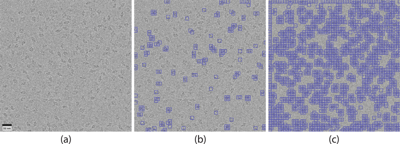
For visualization of our suggested framework, we turn to a micrograph of β-galactosidase (Scheres, 2015; Chen et al., 2013; Scheres and Chen, 2012). We select B = 324 reference images in the manner detailed in Section 2.2, and aim to classify 21904 query images. The query images are selected from locations throughout the micrograph in a way that ensures some overlap between images. For each query image we compute the corresponding response signal according to (4). The threshold t is then computed from all the response signals according to (6). Once this is done, the value k (s_g) is computed for each query image. We present in Fig. 4 a visualization of the results. Since we expect query images that contain particles to be associated with high-valued k (s_g), we present the 1000 query images with highest k (s_g). Fig. 4b shows that, as expected, these regions do contain particles. In addition, we present the 9000 query images with highest k (s_g). The regions not contained in any of these query images are associated with low-valued k (s_g) and can be seen in Fig. 4c to contain no particle.

Fig. 4.

Result of our cross-correlation scheme. (a) Micrograph of β-galactosidase. (b) The 1000 regions contained in boxes have high k(s_g) and are thus regions with a high probability of containing a particle. (c) There are 9000 regions contained in boxes. These regions have high or intermediate k(s_g). Consequently, the regions not contained in boxes have low k(s_g) and thus are likely to be pure noise.

We note that for the sake of reducing the computational complexity of our suggested framework, the cross-correlation score is computed using fast Fourier transforms. This is a well-established method of reducing complexity (Nicholson and Glaeser, 2001).

2.4. APPLE classification

A particle picking framework should produce a single window containing each picked particle. It is possible to use the output of the cross-correlation scheme introduced in Sections 2.1, 2.2, 2.3 as the basis of a particle picker. This is done by defining the query set to be the set of all possible n × n windows contained in the micrograph. The content of each query window is determined according to its score. Specifically, if the score is above a threshold we determine that it contains a particle. This determination can be applied to the location of the central pixel in that window to provide a classification of each pixel in the micrograph (except for boundary pixels that are not in the center of any possible n × n window). Unfortunately, the cost of such an endeavor, both in runtime and in memory consumption, is prohibitive.

In order to improve performance, the APPLE picker does not define the set of query images as all possible n × n windows in the micrograph. Instead, the set of query images ${\left\{h_m\right\}}_{m=1}^C$ is defined as the set of all n × n windows extracted from the micrograph at n/2 intervals. However, applying a determination to the center pixel of each query window will no longer allow for successful particle picking. Indeed, where two overlapping query windows are determined to contain a particle, it is unknown whether they both contain the same particle or whether each contains a distinct particle. It is possible that the interval of n/2 between the query windows caused us to skip over windows that would have been classified as noise. In other words, in order to get a good localization of the particle, the content of each possible window of the micrograph should be determined.

To achieve this, the APPLE picker determines the content of all possible windows in the micrograph via a support vector machine (SVM) classifier. This classifier is based on the mean and variance of windows, which are simple and easily calculated features known to differ between particle regions and noise regions. In this manner we achieve fast and localized particle picking. The classifier is trained on the images whose classification (as particle or as noise) is given with high confidence by our cross-correlation scheme.

To train the classifier, we need a training set. This is composed of a set of examples for the particle images, S₁, and a set of examples for the noise images, S₂. The complete training set is S₁ ∪ S₂. The choice of S₁ and S₂ depends on two parameters, τ₁ and τ₂. These parameters correspond to the percentage of training images that we believe do contain a particle (τ₁) and the percentage of training images that we believe may contain a particle (τ₂).

The selection of τ₁ and τ₂ can be made according to the concentration of the particle projections in the micrograph. This information can be estimated visually at the time of data collection from a set of initial acquired micrographs.

To demonstrate the selection of τ₁ and τ₂, we consider a micrograph with M = 20, 000 query images. If it is known that there is a mid to high concentration of projected particles, we can safely assume that, e.g., 1000 images with highest k (${\mathbf{s}}_{h_m}$) contain a particle. Thus we set τ₁ = 5%. In addition, it is possible that out of 20000 query images 15,000 may contain some portion of a particle. We can therefore safely assume that the regions of the micrograph that are not contained in any of the τ₂ = 75% images with highest k (${\mathbf{s}}_{h_m}$) will be regions of noise.

When the concentration of particle projections is unavailable, the selection of τ₁ and τ₂ can be done heuristically. For instance, τ₁ = 5% and τ₂ = 75% is often a good selection for τ₁ and τ₂. We note that when the concentration of macromolecules is not high, the value of τ₂ is less important than that of τ₁.

Once τ₁ is selected, the set S₁ is determined. Due to the overlapping nature of query images, there is no need to use all τ₁ percent of images with highest k (${\mathbf{s}}_{h_m}$) for training. Instead, we note that these images form several connected regions in the micrograph (see Fig. 4). The set S₁ is made of all non-overlapping windows extracted from these regions.

The τ₂ percent of query images with highest k (${\mathbf{s}}_{h_m}$) form the regions in the micrograph that may contain particles. An example of these regions can be seen in Fig. 4c. The set S₂ is made of non-overlapping windows extracted from the complement of these regions. The reason for the difference between the determination of S₁ and S₂ is that the query images overlap, and we do not want to train the noise model from any section of the τ₂ percent of query images with moderate to high k (s_g).

The training set for the classifier consists of vectors ${\mathbf{x}}_1,\dots ,{\mathbf{x}}_{\left|S_1\cup S_2\right|}\in {\mathbf{ℝ}}_{+}^2$ and labels $y_1,\dots ,y_{\left|S_1\cup S_2\right|}\in \{0,1\}$. Each vector x_i in the training set contains the mean and standard deviation of a window h_i ∈ S₁ ∪ S₂, and is associated with a label y_i, where

$$y_i=\{\begin{array}{ll}1,& \text{if}{h}_i\in S_1.\\ 0,& \text{if}{h}_i\in S_2.\end{array}$$

We note that while training the classifier on mean and variance works sufficiently well, they are not necessarily optimal and other features can be added. This is the subject of future work.

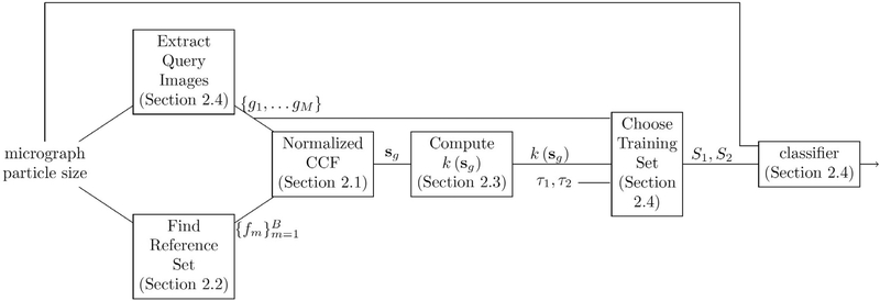
The training set is used in order to train a support vector machine classifier (Schölkopf and Smola, 2001; Cortes and Vapnik, 1995). We propose using a Gaussian radial basis function SVM. Once the classifier is trained, a prediction can be obtained for each window in the micrograph. This classification is attributed to the central pixel of the window, thus classifying each pixel in the micrograph as either a particle or a noise pixel. This provides us with a segmentation of the micrograph. Fig. 1b presents such a segmentation for the micrograph depicted in 1a. For convenience, we summarize our framework in Fig. 5.

Fig. 5.

Overview of APPLE picker

2.5. APPLE picking

The output of the classifier is a binary image where each pixel is labeled as either particle or as noise. Each connected region (cluster) of particle pixels may contain a particle. On the other hand it may contain some artifact. Thus, we disregard clusters that are too small or too big. This is done through examining the total number of pixels in each cluster, and discarding any that are above or below a reasonable number of pixels. This number is selected based on the true particle size.

Alternatively, this can be done through use of morphological operations. An erosion (Efford, 2000) is a morphological operation preformed on a binary image wherein pixels from each cluster are removed. The pixels to be removed are determined by proximity to the cluster boundary. In this way, the erosion operation shrinks the clusters of a binary image. This shrinkage can be used to determine the clusters that contain artifacts. Large artifacts will remain when shrinking by a factor larger than the particle size. Small artifacts will disappear when shrinking by a factor smaller than the particle size. We use this method of artifact removal in the results presented in Section 3. We note that a similar method for contaminant removal was used in AutoPicker (Langlois et al., 2014).

Beyond these artifacts, it is possible that two particles are frozen very close together. This will distort the true particle projection and should be disregarded. For this reason it is good practice to disregard pairs of clusters of pixels that were classified as particle if they are too close. We do this by disregarding clusters whose centers are closer than some distance, for example the particle diameter. We then output a box around the center of each remaining cluster of pixels that were classified as particle. The size of the box is determined according to the known particle size. The pixel content of each box is a particle picked by our framework. See Fig. 1c.

After all particles are picked, it is possible to create templates out of them and use a template matching scheme to pick additional particles, as in (Frank and Wagenknecht, 1983; Ludtke et al., 1999; Scheres, 2015).

2.6. CTF correction

In the process of acquiring the micrograph each particle projection is convolved with a point spread function. This function is the inverse Fourier transform of a function called the contrast transfer function (CTF), which is defined as follows (Mindell and Grigorieff, 2003)

$$\begin{gathered} CTF(g)=-\sqrt{1-A^2}\sin (\chi )-A\cos (\chi ) \\ \chi =\pi \lambda g^2\mathrm{\Delta }f-\frac{\pi }{2}{C}_s{\lambda }^3{g}^4, \end{gathered}$$ (7)

where Δf is the defocus, λ is the wavelength, g is the radial frequency, C_s is the spherical aberration and A is the amplitude contrast.

A well-known effect of the CTF is increasing the support size of the projection image. This effect may cause nearby particle projections to become difficult to distinguish. Another issue is that the CTF decreases the contrast of the projection images, which makes them harder to find. Due to the above, while there is no strict necessity to apply the APPLE picker to CTF-corrected micrographs, it is good practice to do so. The problems of CTF estimation (Rohou and Grigorieff, 2015) and CTFcorrection (Downing and Glaeser, 2008; Turoňová et al., 2017) are well-researched problems. We use CTFFIND4 (Rohou and Grigorieff, 2015) for CTF estimation.

One method of CTF-correction is phase-flipping, which preserves the statistics of the noise, while effectively preventing the CTF from changing sign. While this method does not correct for the amplitude of the CTF, the phase correction already brings the support size close to its true value. It also slightly increases the particle contrast.

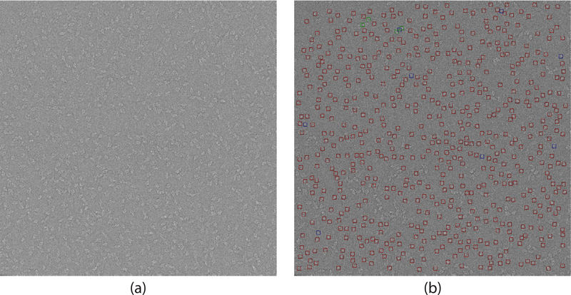
Fig. 6 contains a comparison between our particle picking framework when applied to the micrographs with and without phase-flipping. We mark all particles picked from the micrograph both before and after CTF correction by red squares. We mark the selections made only from the CTF corrected micrograph by green squares. We mark the selections made only from the non CTF corrected micrograph by blue squares. We note that, while most of the picked particles appear in both micrographs, there are slight differences around some of the near-by particles. In particular, Fig. 6 contains a blue square flanked on both sides by green squares. The blue square contains portions of two adjacent particles since the APPLE picker did not successfully separate between both particles. However, after CTF correction each of these particles is selected separately since the APPLE picker was able to distinguish between them. Thus, we recommend this method when applying CTF correction to micrographs before particle picking.

Fig. 6.

Illustration of picking with and without CTF correction. (a) A CTF-corrected β-galactosidase micrograph. CTF estimation was done using CTFFIND4 (Rohou and Grigorieff, 2015) followed by phase-flipping. (b) Results. Particles picked in both micrographs are surrounded by a red box. Selections unique to the phaseflipped micrograph are surrounded by a green box. Selections unique to the original micrograph are surrounded by a blue box. Defocus value for the micrograph is 4191.1 nm.

3. Experimental results

We present experimental results for the framework presented in this paper. We apply our framework to datasets of β-galactosidase, T20S proteasome, 70S ribosome and keyhole limpet hemocyanin (KLH) particles.

The β-galactosidase dataset we use is publicly available from EMPIAR (the Electron Microscopy Public Image Archive) (Iudin et al., 2016) as EMPIAR-10017.⁴ It consists of 84 micrographs of β-galactosidase. The T20S proteasome dataset is publicly available as EMPIAR-10057⁵ (Danev and Baumeister, 2016). It contains 158 micrographs. The 70S ribosome dataset is available as EMPIAR-10077 (Fischer et al., 2016) and contains thousands of micrographs. The KLH dataset we use (Zhu et al., 2004; Zhu et al., 2003) contains 82 micrographs.

The experiments are run on a 2.6 GHz Intel Core i7 CPU with four cores and 16 GB of memory. Our method has also been implemented on a GPU. It is evaluated using an Nvidia Tesla P100 GPU.

3.1. β-galactosidase

We ran the suggested framework on a β-galactosidase dataset (Scheres, 2015). We compare the performance of the APPLE picker to the semi-automated particle picker included in RELION. For this comparison, we input the locations of our picked particles into RELION and obtain a 3D reconstruction. We then compare this to the reconstruction obtained by the full RELION pipeline in (Scheres, 2015).

The β-galactosidase micrographs are obtained using a FALCON II detector. Thus, each micrograph is of size 4096 × 4096 pixels. The outermost pixels in these micrographs do not contain important information. In light of this, when running the APPLE picker on these micrographs, we discard the 100 outermost pixels. In addition, for runtime reduction, each dimension of the micrograph is reduced to half its original size, bringing the micrograph in total to a quarter of its original size. This is done by averaging adjacent pixels, also known as binning.

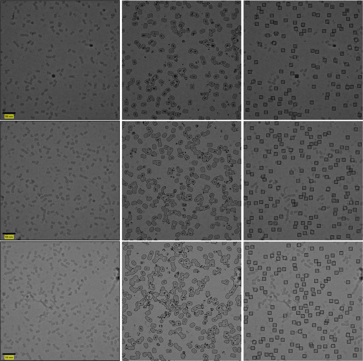
Each query and reference image extracted from the reduced micrograph is of size 26 × 26 and each container is of size 225 × 225. For classifier training we suggest to use τ₁ = 3% and τ₂ = 55% to determine the training set. We set the bandwidth of the kernel function for the SVM classifier and its slack parameter both to 1. Examples of results for the APPLE picker are presented in Fig. 7.

Fig. 7.

Picked particles of sample β-galactosidase micrographs (without CTF correction). The micrographs are presented in the left column. Classification results are presented in the center. The picked particles are on the right. Defocus values are 4191.1, 4859.1 and 4224.8 nm for the top, middle and bottom micrographs, respectively. All defocus values were calculated with ctffind4 from the RELION wrapper.

For the purpose of evaluating our framework, we perform a 3D reconstruction of the particle and compare to the reconstruction of (Scheres, 2015) where the particle picking was done based on 2555 manually selected particles. From these particles, 25 class averages were computed and 10 were manually chosen. The RELION particle picker then picked 52495 particles. Of these, 4185 particles were discarded according to Z-scores. After the class averaging step 42,755 particles were selected. The reported resolution in (Scheres, 2015) is 4.2 Å.

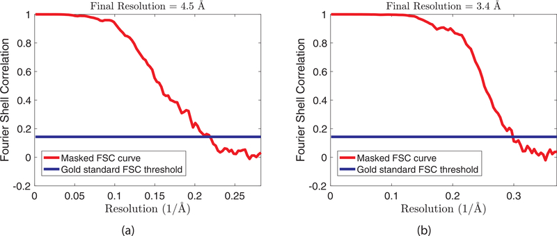
In contrast, we use 32997 particles selected by the APPLE picker. We enter them into the RELION pipeline and begin the reconstruction from our particles. After the 2D class averaging step 15198 particles were selected. The 3D reconstruction using RELION (including CTF correction using the wrapper for CTFFIND4 (Rohou and Grigorieff, 2015)) reached a gold-standard FSC resolution of 4.5 Å.⁶

We present a comparison of surface views from the model reconstructed from particles selected by the APPLE-Picker (in red) and the reconstructed model by (Scheres, 2015) in Fig. 8. These renderings were done in UCSF Chimera⁷(Pettersen et al., 2004). In addition, we present the FSC curve produced by RELION’s post-processing task in Fig. 11.

Fig. 8.

Comparison between the APPLE picker and the RELION semi-automatic particle picker. On the top are surface views of the 3D reconstruction of the β-galactosidase macromolecule created in RELION from the APPLE picks (when picking from CTF corrected micrographs) and obtained in UCSF Chimera. On the bottom are surface views of the 3D views detailed in (Scheres, 2015). We use the reference volume published on EMDB (EMD-2824) and obtain the views in UCSF Chimera.

Fig. 11.

FSC curves as produced by RELION after B-factor sharpening and masking. (a) Curve for the β-galactosidase dataset. (b) curve for the T20S proteasome dataset.

Runtime for a single micrograph is approximately two minutes when running on the CPU. Thus, the entire dataset can be processed in under 3 h. The GPU implementation, on the other hand, takes approximately 8 s. In other words, the APPLE picker processes all 84 micrograph in under 15 min. This is significantly faster than manual picking.

3.2. T20S proteasome

The T20S proteasome (Danev and Baumeister, 2016) dataset is publicly available as EMPIAR-10057. Its micrographs were acquired using a K2 direct detector. Thus, they are sized 3838 × 3710 pixels. Unlike the dataset presented in Section 3.1, this dataset contain elongated particles. In addition, this set was collected using a Volta phase plate at focus. The boost in phase contrast makes particles in these datasets more readily identifiable.

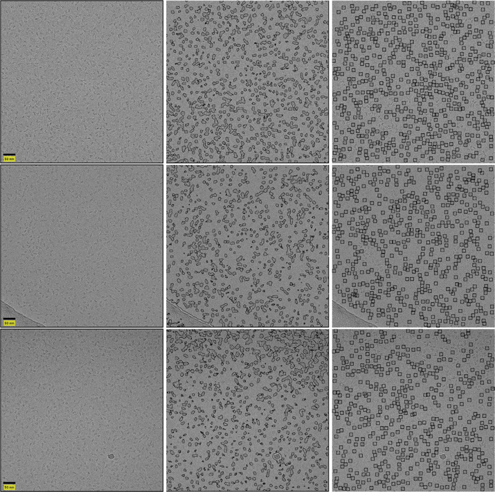
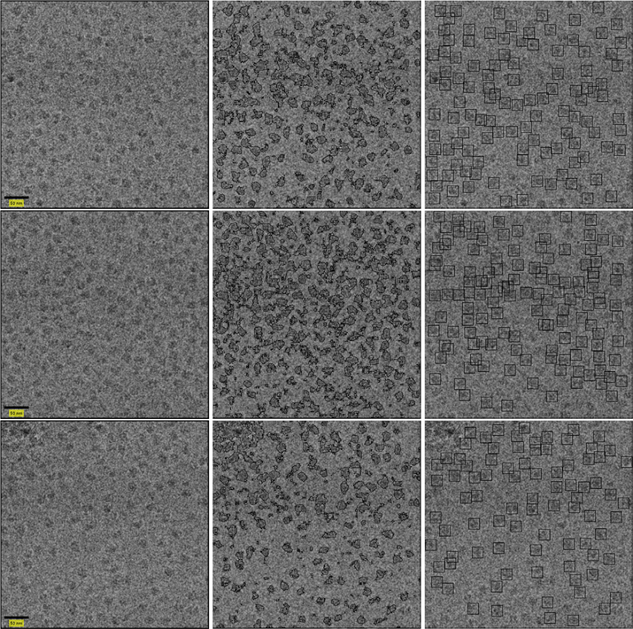
Once again, we use binning to reduce the size of the micrographs. Each query and reference image extracted from the reduced micrograph is of size 24 × 24. We use the same container size, τ_1, τ₂ and SVM classifier parameters as reported in Section 3.1. Examples of results for the APPLE picker are presented in Figure 9.

Fig. 9.

Picked particles of sample T20S proteasome micrographs without CTF correction. The micrographs are presented in the left column. Classification results are presented in the center. The picked particles are on the right.

We first corrected for motion using unblur (Grant and Grigorieff, 2015). We applied the APPLE picker to the motion-corrected micrographs and extracted 21791 particles. These particles were entered into the RELION pipeline. After the class averaging step 15252 particles were selected. The 3D reconstruction of RELION reached a gold-standard FSC resolution of 3.4 Å.

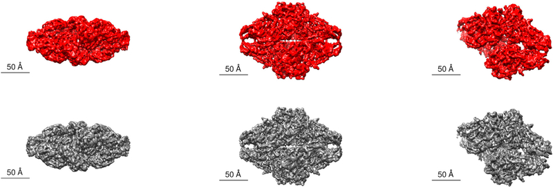
We present a comparison of surface views from the model reconstructed from particles selected by the APPLE picker (in red) and the reconstructed model by (Danev and Baumeister, 2016) in Fig. 10. These renderings were done in UCSF Chimera (Pettersen et al., 2004). In addition, we present the FSC curve produced by RELION’s post-processing task in Fig. 11.

Fig. 10.

Comparison between the APPLE picker and the particles picked in (Danev and Baumeister, 2016). On the top are views of the 3D reconstruction of the T20S proteasome macromolecule created in RELION from the APPLE picks and obtained in UCSF Chimera (when picking from micrographs without CTF correction). On the bottom are views of the 3D reconstruction detailed in (Danev and Baumeister, 2016). We use the reference volume published on EMDB (EMD-3347) and obtain the views in UCSF Chimera.

runtime is approximately 90 s per micrograph when running on a CPU, or 7s per micrograph when running on the GPU.

3.3. 70S ribosome

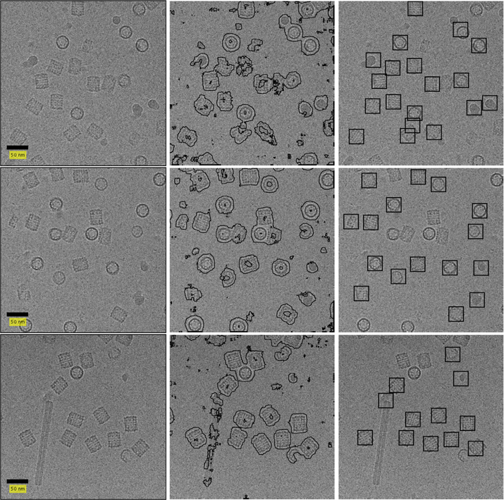
We examine the EMPIAR-10077 (Fischer et al., 2016) dataset. The micrograph are of size 4096 × 4096 and contain large particles. Each query and reference box is of size 40 × 40 pixels in the reduced micrograph. For this reason the container size we use is 500 × 500. This reduces the number of containers and thus causes the number of reference windows to be smaller.

For classifier training we suggest to use τ₁ = 7% and τ₂ = 7% to determine the training set (see Section 4.2 for a discussion about the choice of parameters.) We set the bandwidth of the kernel function for the SVM classifier and its slack parameter both to 1. Examples of results for the APPLE picker are presented in Figure 12. runtime is approximately 2 min per micrograph on the CPU, or approximately 14 s per micrograph on the GPU.

Fig. 12.

Picked particles of sample 70S ribosome micrographs without CTF correction. The micrographs are presented in the left column. Classification results are presented in the center. The picked particles are on the right. Defocus values are 1671.8, 1643.2 and 1595.6 nm for the top, middle and bottom micrographs, respectively.

3.4. KLH

The micrographs in the KLH dataset (Zhu et al., 2004; Zhu et al., 2003) are of size 2048 × 2048. To lower runtime we once again perform binning. Following this reduction in size, we use query and reference images of size 30 × 30 and containers of size 115 × 115. The training set for the SVM classifier is determined using the thresholds τ₁ = 16% and τ₂ = 70%. We use the same configuration of the classifier (bandwidth and slack parameter) as in the previous experiments.

We present in Figs. 13 and 14 some results for the APPLE picker on the KLH dataset. We note these figures show two types of isoforms of KLH. These isoforms are identified in (Roseman, 2004) as KLH1 (short particles) and KLH2 (long particles). We aim to find the KLH1 particles.

Fig. 13.

Result on KLH dataset. The left column contains micrographs without CTF correction. The middle column contains the windows classified as particle by our classifier. The right column contains the picked particles. Defocus values are 4103.6, 1970.2 and 1862.6 nm for the top, middle and bottom micrographs, respectively.

Fig. 14.

Result on KLH dataset. The left column contains micrographs without CTF correction. The middle column contains the windows classified as particle by our classifier. The right column contains the picked particles. Defocus value of the top micrograph is1785.9 nm, middle micrograph1699.3 nm is and bottom micrograph is 1634.3 nm.

As detailed in Section 2.4, we use only mean and variance for classifier training. An issue with this practice is exemplified by the hollow KLH particles. A window containing some regions of the particle and some regions of noise that are internal to the hollow particle is indistinguishable from a window containing some regions of the particle and some regions of noise that are external to the particle. This leads the classifier to identify a ring of pixels around the particle as belonging to the particle. Depending on the concentration of particles in the micrograph, particles may merge together in the output of the classifier.

We use morphological erosion to address this problem. This process, detailed in Section 2.5, will discard all connected components with maximum diameter smaller than 132 pixels and larger than 184 pixels (where the diameter of the KLH particles are approximately 160 pixels). In addition, it will separate adjacent particles connected by a narrow band of pixels. This practice is useful in cases where particle projections are close enough that the rings of pixels around each particle will merge, but distant enough that the merging is restricted to a narrow region between the particles.

Fig. 13 contains micrographs where the particles are either completely isolated or distant enough that the morphological erosion can separate the pixels that were identified as belonging to each of the particles. This is the case in which the APPLE picker is successful despite the hollow particles. Fig. 14 contains micrographs where the particles are clustered closely together, causing the APPLE picker to treat many particles as a single region and thus discard them. It is clear that the APPLE picker is not suited to pick hollow particles that appear with a high concentration. We leave it to future work to solve this issue through addition of more discriminative features to the SVM classifier.

Another issue with the KLH dataset is that different micrographs have vastly different concentrations of particles. This makes it difficult to select a single value of τ₁ that works well on all the micrographs. An example of this is shown in the last row of Fig. 14. When using τ₁ = 5% the APPLE picker performs well on this micrograph.

Our suggested framework processes all 82 micrographs in under 30 min on the CPU and in 4 min on the GPU.

4. Discussion

4.1. A comparison between the APPLE picker and existing particle pickers

Traditionally, cross-correlation based particle pickers can be divided into two groups (Voss et al., 2009). The first of these groups consists of methods that assume templates of the particle are known a priori. This knowledge may exist due to user provided information, projections from some predetermined initial model, etc. The second group imposes mathematical assumptions on the particle.

Obtaining user-provided templates is high in user effort. RELION (Scheres, 2015), for example, necessitates a user to choose 1000–2000 particle projections from several micrographs. This process is costly in both effort and time. Furthermore, user-provided picking introduces a manual bias into the process of particle picking. This bias may cause the templates to be corrupted by bad particle selections. In addition, inexperienced pickers may miss rare views as it is natural for a user to select similar-looking projections. This will exclude certain orientations from the picked particles and adversely affect the achievable resolution.

Beyond the possible issue of manual bias, using templates (userprovided or otherwise) introduces a template bias into the picking process. This was exemplified in (Henderson, 2013), where an image of Einstein was used as the template and matched to random noise. Even though the image was not present in the noise, a reconstruction from the best-matches yielded the original Einstein image. Thus, the template itself may bias the process of particle picking.

The use of mathematical functions as templates can produce good results so long as these functions are a good description of the particle. It should be noted that these mathematical functions are vulnerable to template bias.

In contrast, the APPLE picker does not make assumptions on the structure of the particle. As the APPLE picker uses no templates, requires no manual selection and imposes no assumptions on the particle it is not vulnerable to manual or template bias. We note that, while no assumptions are made on the particle structure, we do assume that the size of the particle is known. In addition, we use the well-established fact that projection images and noise regions differ in their mean intensity and variance. We allow, but do not require, tuning of the parameters τ₁ and τ₂ which are necessary to achieve particle picking in seconds per micrograph. We also allow tuning of maximum and minimum allowed particle size, container size and minimal distance between two projection images.

Another advantage of the APPLE picker is that its reference set contains redundancy (see Section 2.1). This adds a robustness to false positives that is missing from traditional cross-correlation methods.

Thus, the APPLE picker is a simple, robust and fast particle picker which requires low user effort and assumes no prior knowledge of the particle other than its size. The APPLE picker does impose an assumption on the artifacts that may be violated, namely the assumption that the artifact has a different size than the particle projections. If this size assumption is violated, regions containing artifacts can be mistaken for particle projections. However, this can easily be corrected in the 2D classification step.

In recent years there has been increasing interest in the use of deep neural networks for particle picking (Bepler et al., 2018; Tegunov and Cramer, 2018). These networks are in essence classifiers, trained through optimization of a loss (cost) function over a set of positive and negative examples. Typically, the optimization fails to find the global optimum and reaches a local optimum. Despite this, neural networks have proven to be a powerful tool.

Training a deep neural network is a computationally intensive process. Indeed, the training set chosen by the APPLE picker (Section 2.4) could be used for training a deep network. However, our choice of an SVM classifier reduces the complexity of the APPLE picker.

Some deep-learning based particle pickers necessitate manually provided examples for the training. Since the training then proceeds to optimize over these examples, this method is vulnerable to manual bias. In addition this method necessitates high user effort. Other such particle pickers train the neural network on some prior data and then apply it to new datasets. These methods are vulnerable to dataset bias (Torralba and Efros, 2011).

Another advantage of the APPLE picker is that the mathematical theory behind it is simple and clear. On the other hand, the mathematical foundation for deep networks is an active area of study with many open problems.

4.2. Selection of τ₁ and τ₂

In Section 3 we present several datasets with different values of τ₁ and τ₂. For the β-galactosidase and T20S proteasome datasets we use the same values. In this section we explain the difference in values from the 70S ribosome and KLH dataset.

The value of τ₁ determines the percentage of query images that we believe contain a particle. While this value is different between the datasets, the actual number of query images determined by τ₁ is similar for all datasets, and around 500–800. The difference is that the 70S ribosome dataset uses larger query images which causes each micrograph to contain less of them. The KLH micrographs are much smaller than the micrographs of the other datasets and thus, once again, each micrograph contains less query images.

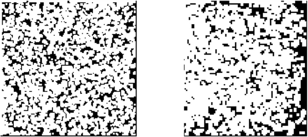
The value of τ₂ is a different matter. Where the query images are large, they tend to cover more of the micrograph.⁸ This may not leave many areas large enough to extract training windows of noise. Thus, we must use smaller values of τ₂. An example of this is presented in Fig. 15 which shows (in white) the locations of the 50% of windows that possess the higher values of k(·) for the β-galactosidase and for the 70S ribosome datasets.

Fig. 15.

Selection of τ₂ for a β-galactosidase sample micrograph (left) and a 70S ribosome sample micrograph (right). The white regions contain the 50% of query images with the highest k(s_g). The black regions are the regions from which the training windows of noise are extracted. We note that while the β-galactosidase sample will have plenty of training windows for noise, the 70S ribosome sample will not.

In conclusion, for micrographs of size 4k × 4k where particles are small and their concentration is similar to that of the micrographs we presented in Section 3, we suggest using τ₂ = 50%−55%. For larger particles we suggest using τ₁ ≈ τ₂. In the future, the APPLE picker’s code will automatically lower τ₂ until a minimal amount of noise training windows are extracted, in which case this issue will no longer be a consideration for the user.

5. Conclusion

In this paper we have presented the APPLE picker, a simple and fast particle picker inspired by template matching. The APPLE picker necessitates no manual particle selection and imposes no assumptions on the particle other than its size. Thus, this framework is unhindered by manual or template bias.

The APPLE picker has two main classification steps. The first step determines the content of query images according to their response to a set of automatically chosen references. While this process is sufficient for particle picking, we achieve a speed-up of our suggested framework when using these results to train a simple classifier.

We presented experimental results on four datasets, and showed the type of particles for which this framework is well suited and the reason our classifier may encounter difficulty. We leave it to future work to solve these issues. We believe that the APPLE picker brings us one step closer towards a fully automated computational pipeline for high throughput single particle analysis using cryo-EM (Baldwin et al., 2018).

References

- Aebeláez P, Han B-G, Typke D, Lim J, Glaeser RM, Malik J, 2011. Experimental evaluation of support vector machine-based and correlation-based approaches to automatic particle selection. J. Struct. Biol 175, 319–328. [DOI] [PubMed] [Google Scholar]
- Baldwin PR, Tan YZ, Eng ET, Rice WJ, Noble AJ, Negro CJ, Cianfrocco MA, Potter CS, Carragher B, 2018. Big data in cryoEM: automated collection, processing and accessibility of EM data. Curr. Opin. Microbiol. 43, 1–8. [DOI] [PMC free article] [PubMed] [Google Scholar]
- Bartesaghi A, Merk A, Banerjee S, Matthies D, Wu X, Milne JLS, Subramanian S, 2015. 2.2 Åresolution cryo-EM structure of β-galactosidase in complex with a cellpermeant inhinitor. Science 348, 1147–1151. [DOI] [PMC free article] [PubMed] [Google Scholar]
- Bepler T, Morin A, Noble AJ, Brasch J, Shapiro L, Berger B, 2018. Positive-unlabeled convolutional neural networks for particle picking in cryo-electron micrographs. In: Research in computational molecular biology, Annual International Conference, RECOMB proceedings RECOMB, pp. 245–247. [PMC free article] [PubMed] [Google Scholar]
- Chen JZ, Grigorieff N, 2007. SIGNATURE: a single-particle selection system for molecular electron microscopy. J. Struct. Biol 157, 168–173. [DOI] [PubMed] [Google Scholar]
- Chen S, McMullan G, Faruqi AR, Murshudov GN, Short JM, Scheres SH, Henderson R, 2013. High-resolution noise substitution to measure overfitting and validate resolution in 3D structure determination by single particle electron cryomicroscopy. Ultramicroscopy 135, 24–35. [DOI] [PMC free article] [PubMed] [Google Scholar]
- Cortes C, Vapnik V, 1995. Support-vector networks. Mach. Learn 20, 273–297. [Google Scholar]
- Danev R, Baumeister W, 2016. Cryo-EM single particle analysis with the Volta phase plate. eLife 5, e13046. [DOI] [PMC free article] [PubMed] [Google Scholar]
- Downing KH, Glaeser RM, 2008. Restoration of weak phase-contrast images recorded with a high degree of defocus: the twin image problem associated with CTF correction. Ultramicroscopy 108, 921–928. [DOI] [PMC free article] [PubMed] [Google Scholar]
- Efford N, 2000. Digital Image Processing: A Practical Introduction Using Java, first ed. Addison-Wesley Longman Publishing Co., Inc., Boston, MA, USA. [Google Scholar]
- Fischer N, Neumann P, Bock LV, Maracci C, Wang Z, Paleskava A, Konevega AL, Schröder GF, Grubmüller H, Ficner R, Rodnina M, Stark H, 2016. The pathway to GTPase activation of elongation factor SelB on the ribosome. Nature 540, 80–85. [DOI] [PubMed] [Google Scholar]
- Frank J, Wagenknecht T, 1983. Automatic selection of molecular images from electron micrographs. Ultramicroscopy 12, 169–175. [DOI] [PubMed] [Google Scholar]
- Grant T, Grigorieff N, 2015. Measuring the optimal exposure for single particle cryo-EM using a 2.6 Å reconstruction of rotavirus VP6. eLife 4, e06980. [DOI] [PMC free article] [PubMed] [Google Scholar]
- Harauz G, Fong-Lochovsky A, 1989. Automatic selection of macromolecules from electron micrographs by component labelling and symbolic processing. Ultramicroscopy 31, 333–344. [DOI] [PubMed] [Google Scholar]
- Henderson R, 2013. Avoiding the pitfalls of single particle cryo-electron microscopy: Einstein from noise. Proc. Nat. Acad. Sci. United States Am 110, 18037–18041. [DOI] [PMC free article] [PubMed] [Google Scholar]
- Hoang TV, Cavin X, Schultz P, Ritchie DW, 2013. gEMpicker: a highly parallel GPUaccelerated particle picking tool for cryo-electron microscopy. BMC Struct. Biol 13, 25. [DOI] [PMC free article] [PubMed] [Google Scholar]
- Iudin A, Korir P, Salavert-Torres J, Kleywegt G, Patwardhan A, 2016. EMPIAR: a public archive for raw electron microscopy image data. Nat. Methods 13. [DOI] [PubMed] [Google Scholar]
- Langlois R, Pallesen J, Ash JT, Ho DN, Rubinstein JL, Frank J, 2014. Automated particle picking for low-contrast macromolecules in cryo-electron microscopy. J. Struct. Biol 186, 1–7. [DOI] [PMC free article] [PubMed] [Google Scholar]
- Ludtke SJ, Baldwin PR, Chiu W, 1999. EMAN: semiautomated software for highresolution single-particle reconstructions. J. Struct. Biol 128, 82–97. [DOI] [PubMed] [Google Scholar]
- McMullan G, Faruqi AR, Clare D, Henderson R, 2014. Comparison of optimal performance at 300 keV of three direct electron detectors for use in low dose electron microscopy. Ultramicroscopy 147. [DOI] [PMC free article] [PubMed] [Google Scholar]
- Mindell JA, Grigorieff N, 2003. Accurate determination of local defocus and specimen tilt in electron microscopy. J. Struct. Biol 142, 334–347. [DOI] [PubMed] [Google Scholar]
- Nicholson WV, Glaeser RM, 2001. Review: automatic particle detection in electron microscopy. J. Struct. Biol 133, 90–101. [DOI] [PubMed] [Google Scholar]
- Ogura T, Sato C, 2004. Automatic particle pickup method using a neural network has high accuracy by applying an initial weight derived from eigenimages: a new reference free method for single-particle analysis. J. Struct. Biol 145, 63–75. [DOI] [PubMed] [Google Scholar]
- Pettersen E, Goddard T, Huang C, Couch G, Greenblatt D, Meng E, Ferrin T, 2004. UCSF Chimera – a visualization system for exploratory research and analysis. J. Comput. Chem 25, 1605–1612. [DOI] [PubMed] [Google Scholar]
- Rohou A, Grigorieff N, 2015. CTFFIND4: fast and accurate defocus estimation from electron micrographs. J. Struct. Biol 192, 216–221. [DOI] [PMC free article] [PubMed] [Google Scholar]
- Roseman A, 2004. FindEM – a fast, efficient program for automatic selection of particles from electron micrographs. J. Struct. Biol 145, 91–99. [DOI] [PubMed] [Google Scholar]
- Scheres SH, 2012. A bayesian view on cryo-EM structure determination. J. Mol. Biol 415, 406–418. [DOI] [PMC free article] [PubMed] [Google Scholar]
- Scheres SH, 2012. RELION: implementation of a Bayesian approach to cryo-EM structure determination. J. Struct. Biol 180, 519–530. [DOI] [PMC free article] [PubMed] [Google Scholar]
- Scheres SH, 2015. Semi-automated selection of cryo-EM particles in RELION-1.3. J. Struct. Biol 189, 114–122. [DOI] [PMC free article] [PubMed] [Google Scholar]
- Scheres SH, Chen S, 2012. Prevention of overfitting in cryo-EM structure determination. Nat. Methods 9, 853–854. [DOI] [PMC free article] [PubMed] [Google Scholar]
- Schölkopf B, Smola AJ, 2001. Learning with Kernels: Support Vector Machines, Regularization, Optimization, and Beyond. MIT Press, Cambridge, MA, USA. [Google Scholar]
- Shatsky M, Hall RJ, Brenner SE, Glaeser RM, 2009. A method for the alignment of heterogeneous macromolecules from electron microscopy. J. Struct. Biol 166, 67–78. [DOI] [PMC free article] [PubMed] [Google Scholar]
- Sigworth FJ, 2004. Classical detection theory and the cryo-EM particle selection problem. J. Struct. Biol 145, 111–122. [DOI] [PubMed] [Google Scholar]
- Tegunov D, Cramer P, 2018. Real-time cryo-EM data pre-processing with Warp. [DOI] [PMC free article] [PubMed]
- Torralba A, Efros AA, 2011. Unbiased look at dataset bias. In: Proceedings of the 2011 IEEE Conference on Computer Vision and Pattern Recognition CVPR ‘ 11, pp. 1521–1528. [Google Scholar]
- Turoňová B, Schur FK, Wan W, Briggs JA, 2017. Efficient 3D-CTF correction for cryo-electron tomography using NovaCTF improves subtomogram averaging resolution to 3.4 Å. J. Struct. Biol 199, 187–195 [DOI] [PMC free article] [PubMed] [Google Scholar]
- van Heel M, 1982. Detection of objects in quantum-noise-limited images. Ultramicroscopy 7, 331–341. [Google Scholar]
- Voss NR, Yoshioka C, Radermacher M, Potter CS, Carragher B, 2009. DoG picker and TiltPicker: software tools to facilitate particle selection in single particle electron microscopy. J. Struct. Biol 166, 205–213. [DOI] [PMC free article] [PubMed] [Google Scholar]
- Wang F, Gong H, Liu G, Li M, Yan C, Xia T, Li X, Zeng J, 2016. DeepPicker: a deep learning approach for fully automated particle picking in cryo-EM. J. Struct. Biol. 195, 325–336. [DOI] [PubMed] [Google Scholar]
- Zhang K, 2017http://www.mrc-lmb.cam.ac.uk/kzhang/.
- Zhu Y, Carragher B, Glaeser RM, Fellmann D, Bajaj C, Bern M, Mouche F, de Haas F, Hall RJ, Kriegman DJ, Ludtke SJ, Mallick SP, Penczek PA, Roseman AM, Sigworth FJ, Volkmann N, Potter CS, 2004. Automatic particle selection: results of a comparative study. J. Struct. Biol. 145, 3–14. [DOI] [PubMed] [Google Scholar]
- Zhu Y, Carragher B, Mouche F, Potter CS, 2003. Automatic particle detection through efficient Hough transforms. IEEE Trans. Med. Imaging 22, 1053–1062. [DOI] [PubMed] [Google Scholar]
- Zhu Y, Ouyang Q, Mao Y, 2016. A deep learning approach to single-particle recognition in cryo-electron microscopy. CoRR, abs/1605.05543. [DOI] [PMC free article] [PubMed] [Google Scholar]