Abstract
Demographic tables are widely used to report baseline characteristics in medical research. However, the traditional copy-paste production method is time-consuming and frequently generates typing errors. Current available statistical tools are still far away from ideal, because they are difficult to understand and they lack flexibility. A user-friendly, dynamic, and flexible tool is needed for researchers to automate the creation of demographic tables. In this paper, we introduce a SAS macro, %ggBaseline, that automatically analyzing and reporting baseline characteristics with the final production of publication-quality demographic tables. The macro provides optional parameters that allow for the full customization of desired demographic tables. Since %ggBaseline allows for the quick creation of reproducible and fully customizable tables, it can be beneficial to academics, clinical trials and medical research studies by making the presentation and formatting of results faster and more efficient.
Keywords: Demographic tables, analyzing and reporting, SAS macro, medical research
Introduction
Demographic information, usually presented in a table and widely used in medical research and population studies, provides a summary of participant characteristics (1,2). A demographic table, usually the first table in a peer-reviewed article on medical research and population studies, is commonly used to describe the population under study and gives the reader a sense of differences in demographic characteristics in the population according to treatment, exposure or outcome (3). A demographic table typically contains summary statistics and P values. Summary statistics often include the counts, means, standard deviations (SD), medians, 25th and 75th percentiles [also called interquartile range (IQR)], and ranges (minimum and maximum values) for continuous variables, and frequencies and percentages of subjects for categorical variables (4). A P value is determined from a statistical test, such as t-test, F-test, or Chi-square test. Table 1 below shows an example demographic table in clinical trials.
Table 1. Example demographic table.
| Variables | Treatment (N=628) | Control (N=372) | P value |
|---|---|---|---|
| Age | <0.0001 | ||
| N (Nmiss) | 628 (0) | 372 (0) | |
| Mean ± SD | 41.6±7.6 | 48.8±7.4 | |
| Min–Max | 29.0–59.0 | 29.0–61.0 | |
| Median (IQR) | 40.5 (35.5–48.0) | 50.0 (44.5–55.0) | |
| Gender (%) | <0.0001 | ||
| Female | 414 (65.9) | 173 (46.5) | |
| Male | 214 (34.1) | 199 (53.5) | |
| Weight | <0.0001 | ||
| N (Nmiss) | 628 (0) | 370 (2) | |
| Mean ± SD | 148.8±26.4 | 157.3±28.3 | |
| Min–Max | 87.0–243.0 | 71.0–250.0 | |
| Median (IQR) | 146.0 (129.5–165.0) | 155.0 (137.0–175.0) |
N, number of non-missing values; Nmiss, number of missing values; SD, standard deviation; IQR, interquartile range.
In order to create a demographic table, one can use statistical software, such as SPSS, SAS, Stata or R to calculate summary statistics and P values, and then copy and paste outputs from statistical software into pre-designed tables in Microsoft Word or Excel or LATEX. However, there are some drawbacks to this process of producing demographic tables. First, it is tedious and time-consuming. Regardless of which software one uses, one must spend a significant amount of time and energy in formatting the results to meet the publication requirement. Second, it is difficult to control the quality and the correctness of results. During this manual copy-paste process, one has to spend a lot of time on double-checking for typographical errors. In addition, this traditional copy-paste method does not comply with the concept of reproducible research (5-7) and literate programming (8) in academia. Although we have a long way to go before fully reaching the standard of reproducible research (9), we can minimize the usage of manual operations by automatically producing demographic tables. Many software engineers, biostatisticians, and medical researchers have attempted to develop command-line interface-based tools that can generate publishable statistical tables directly from research data (10-14). However, these tools are still far from optimal because they are either hard to understand or lack flexibility and thus cannot be applied to a wide variety of situations to create demographic tables for academic journals (12).
SAS, one of the most popular statistical software, has many procedures for obtaining summary statistics and implementing statistical tests. However, none of them can directly generate demographic tables that meet the publication requirement, such as that of the American Psychological Association (APA) style table (2). With some upfront coding work, we can combine SAS features to make a compelling tabulating tool for automatically producing demographic tables. In this paper, we will introduce a powerful SAS macro, %ggBaseline, which can directly produce APA style demographic tables.
Methods
Statistical methods underline demographical tables
Typically, a complete demographic table contains two parts: statistical description and statistical inference. In the statistical description part, depending on the distribution of a continuous variable, mean ± SD and/or median (IQR) will be used to show the central tendency and dispersion. For a categorical variable, it is sufficient to report the frequency and relative percentage of each category. The statistical inference part contains P values from the appropriate statistical tests. The details on the choice of appropriate statistical tests have been discussed in many books (2,4). The primary purpose of demographic tables is to assess group differences in demographic characteristics of the population. Therefore, most of the time, t-test, Wilcoxon rank-sum test, F-test, Kruskal-Wallis test, and Chi-square test would be enough for this purpose. See Table 2 below for more details.
Table 2. Commonly used statistical description and tests for demographic tables.
| Variable | Distribution | Single group | Two groups | Three or more groups |
|---|---|---|---|---|
| Continuous variable | ||||
| Describe | Normal | Mean ± SD | Mean ± SD | Mean ± SD |
| Non-normal | Median (IQR) | Median (IQR) | Median (IQR) | |
| Inference | Normal | NA | t-test/standard difference/Hodges-Lehmann estimator | F-test |
| Non-normal | NA | Wilcoxon rank sum test | Kruskal-Wallis test | |
| Categorical variable | ||||
| Describe | NA | N (%) | N (%) | N (%) |
| Inference | NA | NA | Chi-square test/standard difference | Chi-square test |
SD, standard deviation; IQR, interquartile range; NA, not applicable; N, number of non-missing value; %, percentage.
In medical research and population studies, with a sufficiently large sample, a statistical test will almost always demonstrate a significant difference, unless there is no effect whatsoever. In this situation, the standardized difference would be a useful and straightforward alternative to P values when there are only two groups. Standardized difference scores are intuitive indexes that measure the effect size between two groups. Compared to the t-test or Wilcoxon rank-sum test, they are independent of sample size. An absolute standardized difference greater than 10 percent is approximately equivalent to a P value less than 0.05, which indicates a significant imbalance of a baseline covariate (15-17). This method has been widely used in the literature (18,19). However, the absolute standardized difference can only be calculated for means or percentages. For median, Hodges-Lehmann estimator would be a proper measurement (20).
SAS programming tools for demographical tables
SAS has many functions and procedures for data manipulation, statistical description and inference, and data presentation. The SAS procedures PROC TABULATE and PROC REPORT can generate descriptive statistical tables. However, no procedure is available to accomplish an APA style demographic table in one step. The most appropriate strategy is to assemble procedures that produce descriptive statistics and P values, as well as other entries in the demographic table by packing them into a user-friendly SAS macro. A SAS macro is a set of SAS data step statements and procedures that can perform some specific task efficiently. It is often used to reduce the amount of regular SAS code and provides an efficient way to automate a process.
To develop a user-friendly SAS macro that can automatically produce publishable demographic tables, we need to perform at least four steps. First, we use statistical procedures to get descriptive and inferential statistics. PROC MEANS and PROC FREQ are the ideal SAS procedures for obtaining descriptive statistics (N, Nmiss, Mean, SD, Median, IQR, Min, Max, frequency, and percentage). Inferential statistics (P value of t/F/Chi-square/Wilcox/Kruskal Wallis test) can be obtained through SAS procedures PROC TTEST/ANOVA/FREQ or PROC NPAR1WAY. Next, we apply data manipulation statements/functions and procedures to merge descriptive and inferential statistics into one dataset that is applied to PROC REPORT procedure. Data step functions such as CATS, output delivery system (ODS) statement such as ODS OUTPUT, data manipulation procedures such as PROC TRANSPOSE, and even rich text format (RTF) code will be required to complete this task. Then, we run PROC REPORT and ODS statements to generate the desired table in an RTF or PDF file. Lastly, we adapt the SAS code snippets into sub-macros, and then put the sub-macros together into a powerful macro that can be reused in the near future. We can also check the correctness of the data, including the existence of the dataset and variables. If the names of a dataset or variables are incorrectly entered, the macro should return error messages. With the utilization of ODS style templates, PROC REPORT, specific RTF codes, and the macro language, we can build a powerful, easy-to-use, dynamic, and flexible SAS macro.
The SAS macro: %ggBaseline
The SAS macro %ggBaseline is a dynamic and flexible SAS reporting tool. It can quickly produce demographic tables for both journal articles and statistical reports for clinical trials. This macro has the following features: (I) it is automatic: it can generate a publishable table from raw data with one click; (II) it is complete: it can automatically produce both descriptive statistics for all variables and P values from parametric tests and non-parametric tests; (III) it is dynamic: with the parameters specified by users, it is easy and efficient to set the variables labels, table title, footnote, statistical test, total column (yes or no), percentage type (row or column percentage), page orientation (portrait or landscape) and document format (RTF or PDF) that allow for the full customization of desired demographic tables; (IV) it is robust: when we run the macro, it performs error processing. It will return error messages when the name of a dataset or variable is incorrectly entered.
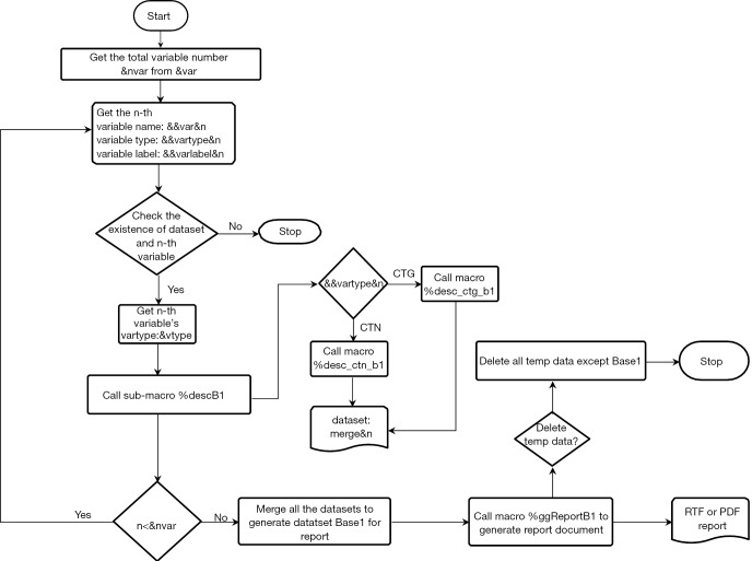
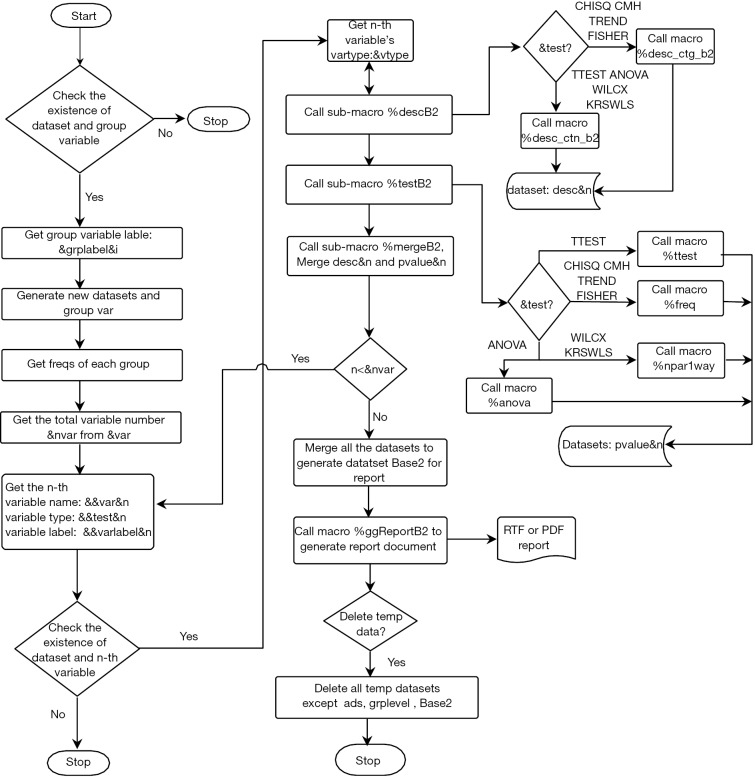
The SAS macro %ggBaseline consists of two sub-macros, %ggBaseline1 and %ggBaseline2, which can generate demographic tables with a single group and multiple groups, respectively. The detailed flow charts of %ggBaseline1 and %ggBaseline2 are shown in Figures 1 and 2.
Figure 1.
Flowchart of the SAS sub-macro %ggBaseline1.
Figure 2.
Flowchart of the SAS sub-macro %ggBaseline2.
Table 3 lists all the parameters and descriptions for the SAS macro %ggBaseline. There are four required parameters (data, var, file, and title) for the demographic tables with one group and six required parameters (data, var, grp, grplabel, file, and title) for the demographic tables with multiple groups. The other nine optional parameters can be specified by users or left blank.
Table 3. The full list of parameters in the SAS macro %ggBaseline.
| Parameter | Instruction |
|---|---|
| Required parameter | |
| data= | Dataset we used |
| var= | Variables we want to list in the table. For a variable, the form should be “variable_name|test_name|variable_label\,” “|” is used as a separator of the variable name, statistical test, and variable label, and “\” is used as a separator between variables. For the last variable, please drop the slash (\) sign. The test name can be TTEST or WILCX when only two groups, and ANOVA or KRSWLS when more than two groups for continuous variables; CHISQ, CMH, TREND or FISHER for categorical variables |
| grp= | Group variable |
| grplabel= | Label for each group level. If we have two groups, treatment and control, then we can set the grplabel parameter as “Treatment|Control”; “|” is used as a separator between labels |
| file= | Specify the file location |
| title= | Specify the table title |
| Optional | |
| stdiff= | Use Y or N to indicate whether we need standard difference to assess variables balance between groups. This parameter is only effected when we have two groups. The default value is N |
| totcol= | Use Y or N to indicate whether we need a total column ahead of group columns. The default value is N |
| pctype= | Use COL or ROW to indicate whether we need a column percentage or row percentage for each categorical value. The default value is COL |
| filetype= | Use RTF or PDF to indicate whether to generate tables in RTF file or PDF file. The default value is RTF |
| footnote= | Specify the footnote under the table |
| fnspace= | Specify the space ahead of footnote |
| page= | Use PORTRAIT or LANDSCAPE to set the page orientation. The default value is PORTRAIT |
| exmissing= | Use Y or N to indicate whether to exclude observations with missing value when calculate percentage. The default model will count the frequency of missing values, but percentage calculation and the statistical test will be based on completed data |
| deids= | Use Y or N to indicate whether to delete intermediate dataset. The default value is Y |
For the demographic tables with a single group, four required parameters (data, var, file, and title) must be specified by users while for the demographic tables with multiple groups six required parameters (data, var, grp, grplabel, file and title) must be specified by users. Nine optional parameters can be specified by users or left blank.
To use %ggBaseline, we first need to pass our macro statements to the macro processor and then call this macro in SAS. The detailed demonstration will be given through working examples in the next section. Here we illustrate the general principle on how to use it. Suppose the macro ggBaseline.sas and two sub-macros ggBaseline1.sas and ggBaseline2.sas are located in the folder of “D:\mymacro”. We can run the following SAS statement to define the %ggBaseline macro. All the source code of SAS macros can be obtained on request at guhongqiu@yeah.net.

After the macro has been defined, we can invoke the macro as follows to generate the desired tables.

Working examples
We will use the “Heart” dataset to illustrate how to use the SAS macro %ggBaseline to automatically generate demographic tables. The “Heart” dataset is available in the SAShelp library of SAS. It contains 5,209 observations and 17 variables from Framingham Heart Study (21). For the purpose of demonstration, we only use five variables in this study, including age (AgeAtStart), sex (sex), weight (Weight), blood pressure status (BP_status), and smoking status (Smoking_Status).
Generating a demographic table with P values
Suppose we want to generate a demographic table with the group variable sex and use P values to evaluate the group differences of three variables, age, weight, and smoking status. We can do it quickly with the following SAS code and obtain a APA-style demographic table in an RTF file named “output1.RTF” in the folder of “D:\mymacro\”.
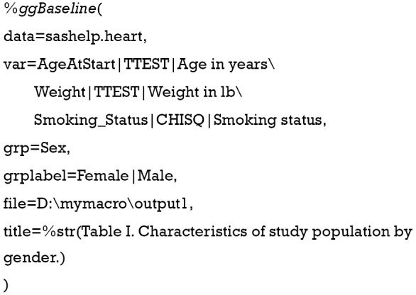
Compared to traditional SAS code, the above macro code is clean and concise. Each variable is followed by the associated statistical test and variable label. Figure 3 shows the resulting table. Each entry in this table is editable and can be easily adapted to meet journal requirements.
Figure 3.
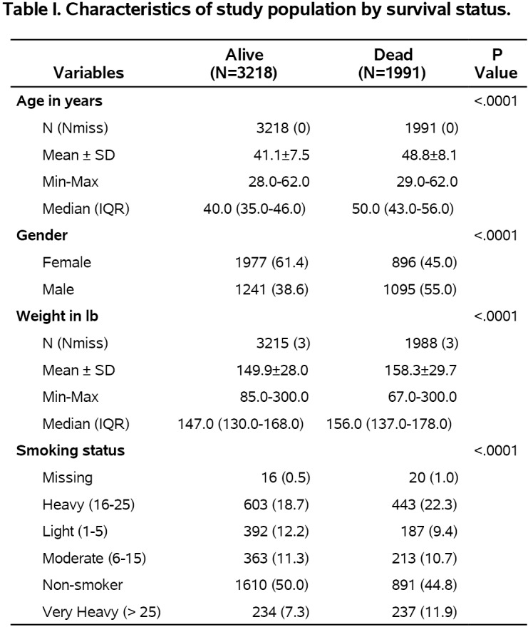
The demographic table with P values generated by the first code in section “Generating a demographic table with P values”.
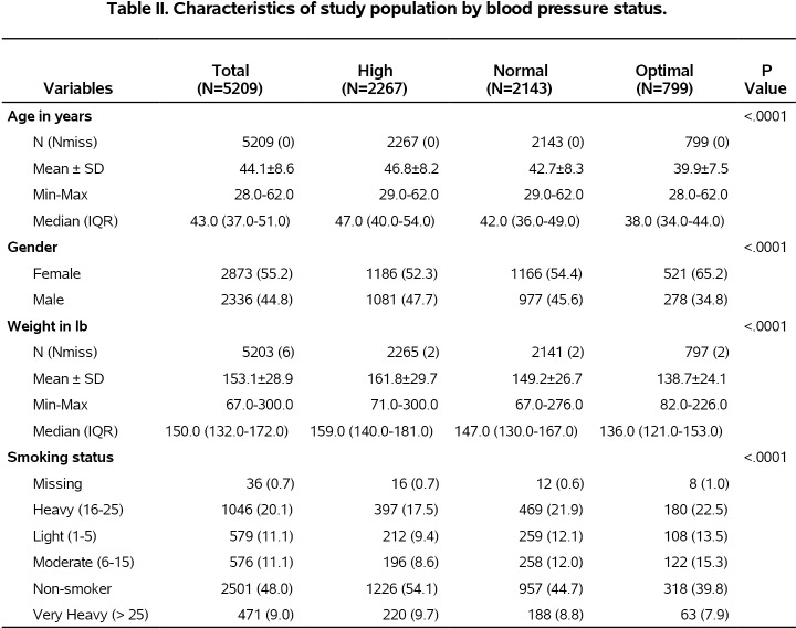
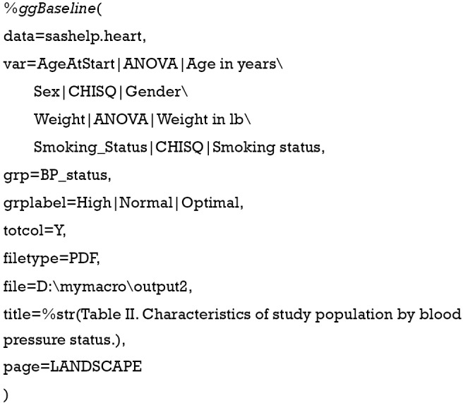
We can use optional parameters listed in Table 3 to make further customization. For example, we can change the group variable from survival status (status) to blood pressure status (BP_status), add a total column, set the page orientation to landscape, and save the resulting table in a PDF file “output2.PDF” in the folder of “E:\mymacro\”. See Figure 4 for the corresponding output.
Figure 4.
The demographic table with P values generated by the second code in section “Generating a demographic table with P values”.
Generating a demographic table with standard differences
As stated in section “Methods”, the standardized difference is desired in some applications. With the optional parameter stdiff=Y, the %ggBaseline macro can also add the standardized difference in the demographic table. Hodges-Lehmann estimator will be given in line with median (IOR) as well. The output is shown in Figure 5.
Figure 5.
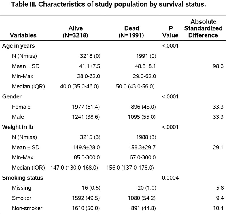
The demographic table with standardized difference generated by the code insection “Generating a demographic table with standard differences”.
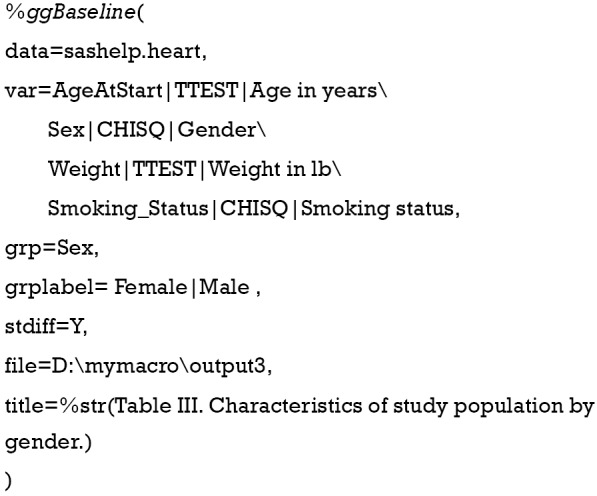
Generating a demographic table without the group variable
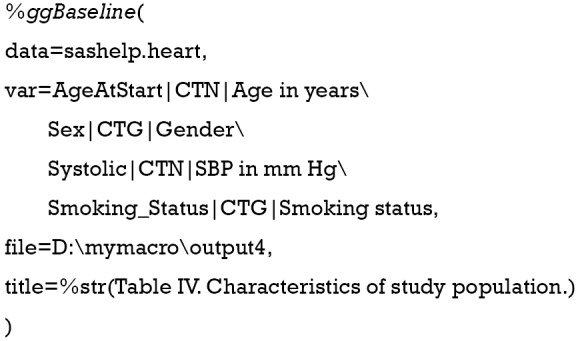
Sometimes, we may need to report the population information without group variables, which means that we treat all the subjects as a single group. In this case, the parameters grp and grplabel are not required in the SAS macro %ggBaseline. In addition, the statistical test should be replaced by variable type (CTN: continuous, CTG: categorical). The following code shows one example of this application. The output is shown in Figure 6.
Figure 6.
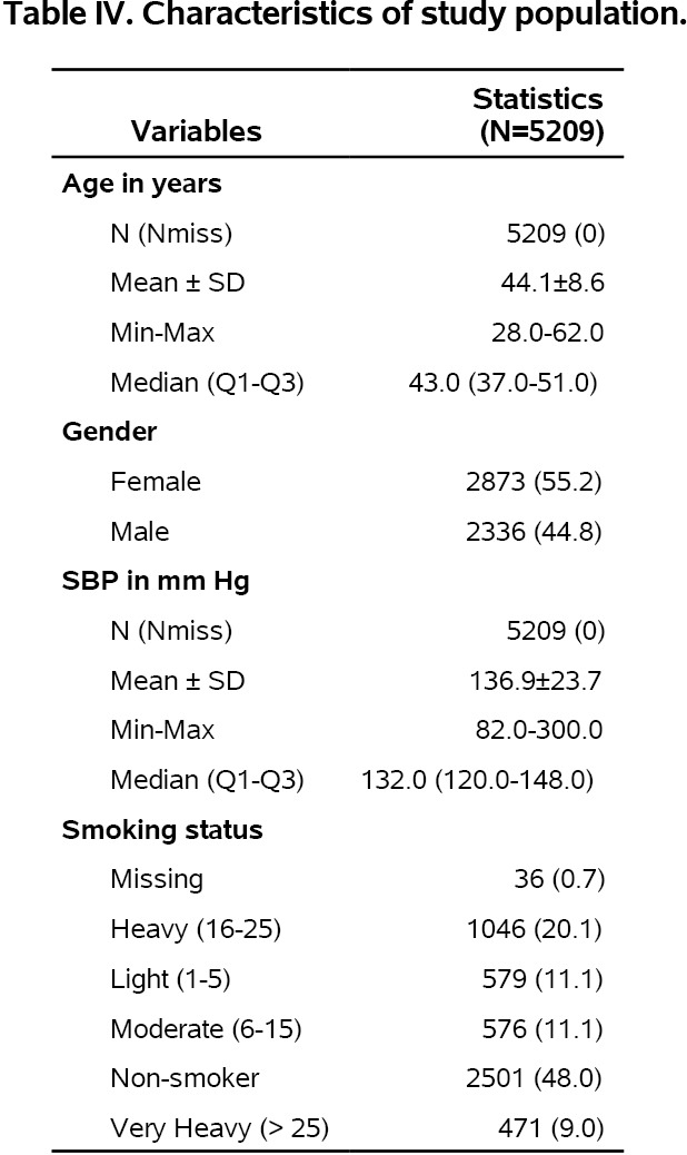
The demographic table without group variables generated by the code in section “Generating a demographic table without the group variable”.
Generate a demographic table using user-defined formats
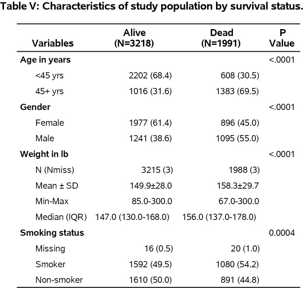
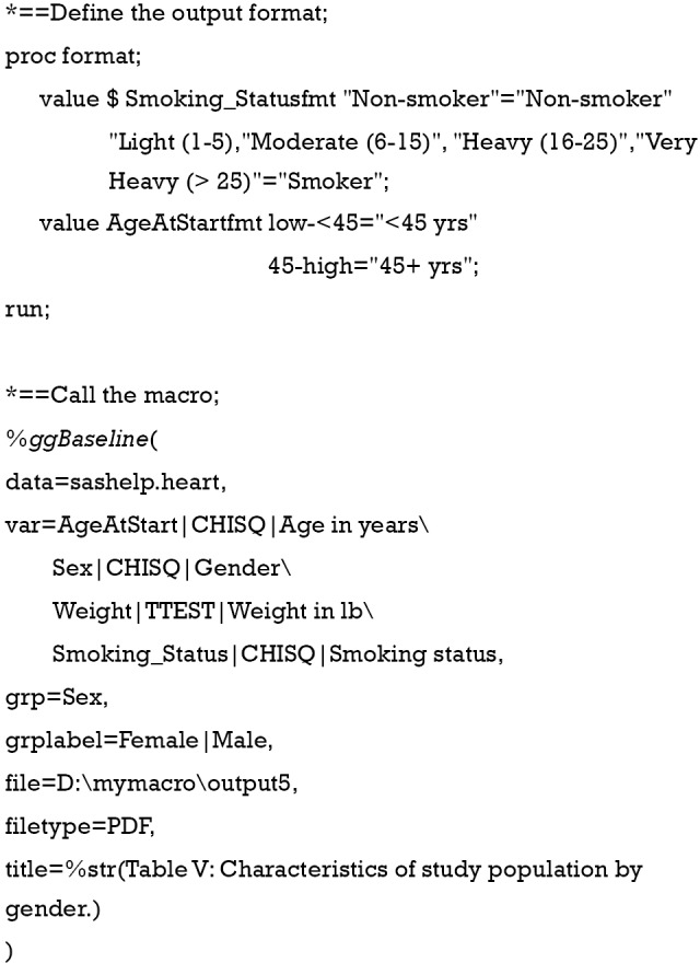
If there are many levels for one categorical variable (for example, zip codes), one may want to reduce the number of levels of this variable by merging some levels together when producing a demographic table. One can use DATA step statements in SAS to create a new categorical variable and then produce a demographic table based on the new categorical variable. However, our SAS macro %ggBaseline can generate the same demographic table without creating a new categorical variable. What we need to do is to change the output format by adding the suffix “fmt” to the end of the variable name. For example, there are five levels, “non-smoker”, “light [1–5]”, “moderate [6–15]”, “heavy [16–25]”, “very heavy [>25]”, for the smoking status (Smoking_Status) in the “Heart” dataset. If we want to produce a demographic table that includes only two levels “smoker” and “non-smoker” for the smoking status, we can use the following SAS code to change the output format without creating a new categorical variable. This feature also works for cutting continuous variables into different categories, what we need to do is change the statistical test parameter to CHISQ after defining the format. See Figure 7 for the corresponding output.
Figure 7.
Output generated by the code in section “Generate a demographic table using user-defined formats”.
Discussion
In this article, we have introduced the SAS macro %ggBaseline. The SAS macro %ggBaseline is a powerful tool for biostatisticians and medical researchers to automatically generate publication-quality demographic tables for academic journals and clinical trial statistical reports. The macro allows for the quick creation of reproducible and fully customizable tables. In addition, it allows users to save tables in two different formats, and thus makes all table layouts easily reproducible and transferable.
In conclusion, SAS macro %ggBaseline can offer significant benefits to academics, medical researchers and policy-makers. It can significantly enhance the speed and efficiency of report creation and presentation, and thus save valuable time that can be allocated to other productive tasks.
Acknowledgements
Funding: HQ Gu was supported by Youth Science Funding of Beijing Tiantan Hospital (Grant ID: 2016-YQN-07). DJ Li was partially supported by University of Central Florida In-House Research Grant.
Footnotes
Conflicts of Interest: The authors have no conflicts of interest to declare.
References
- 1.Nicol AAM, Pexman PM. Displaying your findings: a practical guide for creating figures, posters, and presentations. American Psychological Association, 2010. [Google Scholar]
- 2.Nicol AAM, Pexman PM. Presenting your findings: a practical guide for creating tables. American Psychological Association, 2010. [Google Scholar]
- 3.Farland LV, Correia KF, Wise LA, et al. P-values and reproductive health: what can clinical researchers learn from the American Statistical Association? Hum Reprod 2016;31:2406-10. 10.1093/humrep/dew192 [DOI] [PMC free article] [PubMed] [Google Scholar]
- 4.Rosner B. Fundamentals of biostatistics. Cengage Learning, 2015. [Google Scholar]
- 5.Atmanspacher H, Maasen S. Reproducibility: principles, problems, practices, and prospects. Wiley, 2016. [Google Scholar]
- 6.Stodden V, Leisch F, Peng RD. Implementing reproducible research. Taylor & Francis, 2014. [Google Scholar]
- 7.Peng RD. Reproducible research and biostatistics. Biostatistics 2009;10:405-8. 10.1093/biostatistics/kxp014 [DOI] [PubMed] [Google Scholar]
- 8.Knuth DE. Literate programming. The Computer Journal 1984;27:97-111. 10.1093/comjnl/27.2.97 [DOI] [Google Scholar]
- 9.Munafò MR, Nosek BA, Bishop DVM, et al. A manifesto for reproducible science. Nature Human Behaviour 2017;1:0021. [DOI] [PMC free article] [PubMed]
- 10.Gandrud C. Reproducible research with R and R studio, Second Edition. CRC Press, 2016. [Google Scholar]
- 11.Xie Y. Dynamic documents with R and knitr, Second Edition. CRC Press, 2015. [Google Scholar]
- 12.Gravely A, Clothier B, Nugent S. Creating an easy to use, dynamic, flexible summary table macro with P-values in SAS for research studies. Chicago: MWSUG, 2014. [Google Scholar]
- 13.Dan R, Feaster D. Using the SAS ODS report writing interface to create clinical study report. SAS Global Forum 2012, Florida 2012. [Google Scholar]
- 14.Kadziola Z. An easy-to-use SAS table formatting macro: stand-alone, flexible, and quick SUGI30. Philadelphia, 2005. [Google Scholar]
- 15.Austin PC. Using the standardized difference to compare the prevalence of a binary variable between two groups in observational research. Commun Stat Simul Comput 2009;38:1228-34. 10.1080/03610910902859574 [DOI] [Google Scholar]
- 16.Fogarty CB, Mikkelsen ME, Gaieski DF, et al. Discrete optimization for interpretable study populations and randomization inference in an observational study of severe sepsis mortality. J Am Stat Assoc 2016;111:447-58. 10.1080/01621459.2015.1112802 [DOI] [Google Scholar]
- 17.Morgan KL, Rubin DB. Rerandomization to balance tiers of covariates. J Am Stat Assoc 2015;110:1412-21. 10.1080/01621459.2015.1079528 [DOI] [PMC free article] [PubMed] [Google Scholar]
- 18.Li F, Morgan KL, Zaslavsky AM. Balancing covariates via propensity score weighting. J Am Stat Assoc 2016;1-11. [Google Scholar]
- 19.Xian Y, Holloway RG, Chan PS, et al. Association between stroke center hospitalization for acute ischemic stroke and mortality. JAMA 2011;305:373-80. 10.1001/jama.2011.22 [DOI] [PMC free article] [PubMed] [Google Scholar]
- 20.Hollander M, Wolfe D A. Nonparametric statistical methods. Wiley, 1999. [Google Scholar]
- 21.Dawber TR, Meadors GF, Moore FE. Epidemiological approaches to heart disease: the Framingham study. Am J Public Health Nations Health 1951;41:279-81. 10.2105/AJPH.41.3.279 [DOI] [PMC free article] [PubMed] [Google Scholar]


