The Importance of the Baby Boom Cohort and the Great Recession in Understanding Age, Period, and Cohort Patterns in Happiness

Abstract

Twenge, Sherman, and Lyubomirsky (TSL) claim that long-term cultural changes have increased young adults’ happiness while reducing mature adults’ happiness. To establish their conclusion, TSL use trend analyses, as well as more sophisticated mixed-effects models, but their analyses are problematic. In particular, TSL’s trend analyses ignore a crucial cohort effect: well-known lower happiness among baby boomers. Furthermore, their data aggregation obscures the ephemerality of a recent period effect: the Great Recession. Finally, TSL overlook a key finding of their mixed-effects models that both pre- and post-Boomer cohorts became happier as they aged from young to mature adults. Our reanalyses of the data establish that the Baby Boomer cohort, the short-lived Great Recession, and unfortunate data aggregation account for TSL’s results. The well-established, long-term relationship between age and happiness remains as it has been for decades despite any cultural shifts that may have occurred disfavoring mature adults.

A recent paper by Twenge, Sherman, and Lyubomirsky (TSL, 2016) presents a startling conclusion. The authors conclude that there is a long-term declining trend in mature adults’ happiness vis-à-vis young adults, and, correspondingly, that the correlation between age and happiness has disappeared in recent years. The authors suggest that this finding reflects that cultural changes between the 1970s and the 2010s have not been favorable to mature adults, but have been to young adults, and that this pattern may be expected to continue.

This conclusion is striking from both substantive and methodological perspectives. From a substantive perspective, there is arguably little in recent history to suggest that conditions have improved for young adults so as to warrant a growth in their happiness vis-à-vis mature adults. For example, an increasing proportion of the U.S. budget is spent on Social Security and Medicare, which has led politicians to issue dire warnings about the future of these programs and the costs to young workers of supporting the aging population (Blendon & Benson, 2011). At the same time, job prospects for young adults have been poor since the recession of 2007. Home ownership rates for young adults are low, and their starting salaries are low. Additionally, fertility levels remain low in the United States, possibly reflecting a decline in children’s value to adults relative to their cost (see Nauck, 2014).

From a methodological perspective, the authors’ conclusion is striking because they rely on analytic techniques that are insufficiently complex (e.g., mean happiness trends and bivariate correlations between age and happiness) for establishing their major conclusion, while presenting mixed-effects regression analyses that, in fact, yield a different conclusion from the one they emphasize based on the simpler methods.

TSL conduct two sets of analyses, including (1a) trend analyses of mean happiness by age-group (young vs. mature adults) and (1b) of the bivariate correlation between age and happiness and (2a) mixed-effects regression analyses (hierarchical age– period–cohort analysis [HAPC]) with main effects for age, period, and cohort for the entire adult age range (i.e., 18 years and older) and (2b) separate models for young and mature adults. In subsequent sections, we replicate these analyses and extend them to show why they are problematic. We argue that the conclusions reached by TSL are a reflection of two unique features of American demography and economics—the Baby Boom cohort and the recent Great Recession—coupled with their method for aggregating the data, and not a general trend toward decreasing happiness of mature adults relative to young adults. In short, while the Boomers and Recession, coupled with TSL’s particular data structure and analytic approach, account for their results, their general conclusion that we are seeing a long-term change is wrong.

Replication and Additional Analyses

Trend analyses of mean happiness for young and mature adults

TSL argue that the trend in the relationship between age and happiness is negative, declining from being a positive relationship previously, and they conclude that the association has disappeared in recent years. The authors first claim that happiness among mature adults has consistently declined, while happiness among young adults has possibly increased. To support this claim, they plot age-group trends in mean happiness across a 43-year period (from 1972 to 2014 using General Social Survey [GSS] data), with periods arbitrarily aggregated into approximate 5-year groupings. We replicated this figure¹ and reanalyzed age-group mean happiness trends and find three shortcomings of TSL’s analyses of these data.

First, the authors’ trend analysis ignores well-known cohort effects. In particular, baby boomers have been recognized, for nearly 40 years (see Easterlin, 1980), to be less happy than other birth cohorts (see Fukuda, 2013; Yang, 2008). Born during the post-WWII period (i.e., 1946–1964), which was characterized by significantly higher total fertility rates than observed in adjacent cohorts, the Boomer cohort is understood to be less happy than other cohorts because of its relatively large size and resulting increased competition for social and economic resources (see Easterlin, 1980). For example, a large cohort creates more competition for entry into schools and the labor market, which leads to negative consequences for expected socioeconomic achievement and family life (Yang, 2008). These unique experiences in early life and young adulthood can have a lasting impact on psychological well-being (see Ryder, 1965; Schaie, 1965). Moreover, boomers’ relatively lower happiness levels, compared to cohorts that came either before or after them, have been consistently evidenced across numerous studies employing various age–period–cohort (APC) modeling techniques (see Fukuda, 2013).

This ubiquitous finding provides sufficient reason to question whether any change in the age–happiness pattern across time truly reflects long-term period change or whether it simply reflects a temporary phenomenon attributable to the baby boomers aging through the life course. In fact, TSL recognize this dilemma in stating that

If, for example, baby boomers (born 1946–1964) are (and were) less happy than other generations, happiness might increase among adolescents as boomers left those age groups and decline among older adults as boomers entered those age groups. (p. 132)

Yet, their trend analyses focus on age and period but ignore cohort. Therefore, we separate boomers from non-boomers in Figure 1b and find that this cohort is driving the declining trend in mature adults’ happiness. In fact, non-boomer mature adults’ happiness appears to increase until about 2000, which significantly challenges the authors’ conclusion that “cultural changes between the 1970s and the 2010s appear to have had … a negative impact on the SWB [happiness] of adults over age 30” (p. 139).

Figure 1.

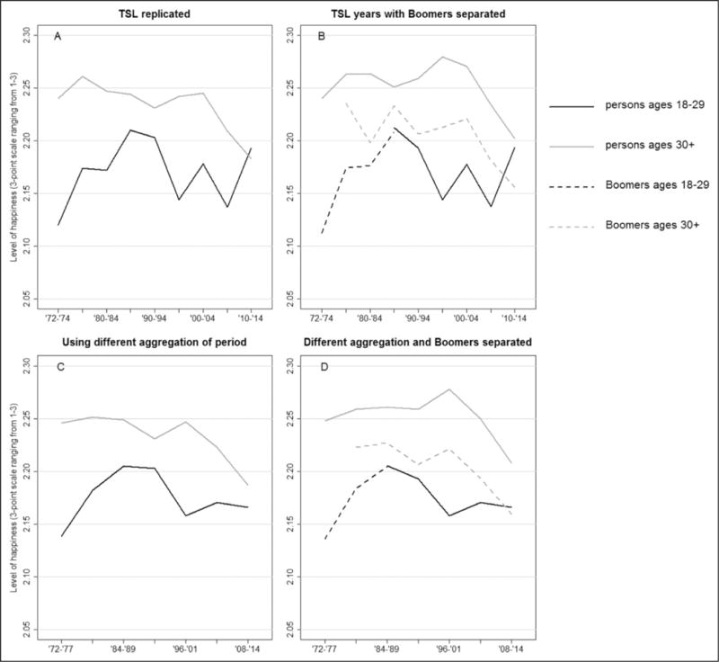
Average levels of happiness among 18- to 29-year-old adults and adults aged 30 and over by time period. The 1982 and 1987 Black oversamples were removed, and the WTSSALL weight variable was used; Boomers include those born between 1945 and 1964, which includes an additional year (i.e., 1945) of birth than normally recognized by demographers, but this year range was selected to match TSL’s 5-year birth cohorts used in mixed regression analyses; see Table 1 for 95% confidence bounds.

Second, TSL’s aggregation of the most recent GSS waves includes two groupings of years that overlap with the Great Recession and its immediate aftermath (i.e., 2005–2009 and 2010–2014)—a particularly important time period to consider in investigating happiness trends (see D. N. Bell & Blanch-flower, 2011). Although TSL justify aggregating the data by saying: “We felt that separating the data into 5-year intervals provided the best compromise between specificity and breadth” (p. 133), and grouping data or using other smoothing methods is often reasonable for illustrating trends, in this case, such aggregation significantly distorts the true underlying pattern in the original data.

We reaggregated survey waves so that the Great Recession years were grouped into a single period (i.e., 2008–2014), an arguably more meaningful division of GSS waves but which also fits with TSL’s approximate 5-year grouping strategy (see Figure 1c and d). Figure 1c shows that, when the Great Recession is isolated, both mature and young adults’ happiness declines during the period, albeit mature adults’ happiness declines more consistently and at a slightly steeper rate than that for young adults. This finding contradicts at least one of TSL’s conclusions—increased happiness for young adults. Moreover, when boomers are separated, as shown in Figure 1d, there is a substantial difference between mature non-boomer adults’ and young adults’ happiness across most time periods (see also Table 1). This result further suggests that boomers, rather than long-term cultural shifts, are driving the declining trend in mature adults’ happiness. Our reanalyses also show that aggregating these data is problematic, especially in the years following the Great Recession (i.e., 2008–2014).

Table 1.

Means and 95% Confidence Bounds for Trend Analyses of Age-Group Happiness—General Social Survey 1972–2014.

Figure 1a	‘72–’74	‘75–’79	‘80–’84	‘85–’89	‘90–’94	‘95–’99	‘00–’04	‘05–’09	‘10–’14
18–29 years	2.12	2.17	2.17	2.21	2.20	2.14	2.18	2.14	2.19
Lower bound	2.08	2.14	2.14	2.18	2.17	2.11	2.14	2.10	2.16
Upper bound	2.16	2.20	2.20	2.24	2.23	2.18	2.21	2.18	2.23
30 and over years	2.24	2.26	2.25	2.24	2.23	2.24	2.25	2.21	2.18
Lower bound	2.22	2.24	2.23	2.23	2.22	2.22	2.23	2.19	2.16
Upper bound	2.26	2.28	2.27	2.26	2.25	2.26	2.26	2.23	2.20
Figure 1b	‘72–’74	‘75–’79	‘80–’84	‘85–’89	‘90–’94	‘95–’99	‘00–’04	‘05–’09	‘10–’14
18–29 years B	2.11	2.17	2.18	2.21	NA	NA	NA	NA	NA
Lower bound	2.07	2.14	2.14	2.17	NA	NA	NA	NA	NA
Upper bound	2.15	2.21	2.21	2.24	NA	NA	NA	NA	NA
18–29 years NB	NA	NA	NA	2.21	2.19	2.14	2.18	2.14	2.19
Lower bound	NA	NA	NA	2.16	2.16	2.11	2.14	2.10	2.16
Upper bound	NA	NA	NA	2.27	2.23	2.18	2.21	2.18	2.23
30 and over years B	NA	2.24	2.20	2.23	2.21	2.21	2.22	2.18	2.16
Lower bound	NA	2.17	2.16	2.21	2.19	2.19	2.20	2.15	2.13
Upper bound	NA	2.30	2.23	2.26	2.23	2.24	2.25	2.21	2.18
30 and over years NB	2.24	2.26	2.26	2.25	2.26	2.28	2.27	2.23	2.20
Lower bound	2.22	2.24	2.24	2.23	2.24	2.25	2.25	2.21	2.18
Upper bound	2.26	2.28	2.29	2.27	2.28	2.31	2.30	2.26	2.22
Figure 1c	‘72–’77	‘78–’83	‘84–’89	‘90–’95	‘96–’01	‘02–’07	‘08–’14
18–29 years	2.14	2.18	2.20	2.20	2.16	2.17	2.17
Lower bound	2.11	2.15	2.17	2.17	2.13	2.13	2.14
Upper bound	2.17	2.21	2.23	2.23	2.19	2.21	2.20
30 and over years	2.25	2.25	2.25	2.23	2.25	2.22	2.19
Lower bound	2.23	2.23	2.23	2.21	2.23	2.20	2.17
Upper bound	2.27	2.27	2.27	2.25	2.27	2.24	2.21
Figure 1d	‘72–’77	‘78–’83	‘84–’89	‘90–’95	‘96–’01	‘02–’07	‘08–’14
18–29 years B	2.14	2.18	2.20	NA	NA	NA	NA
Lower bound	2.11	2.15	2.17	NA	NA	NA	NA
Upper bound	2.17	2.21	2.23	NA	NA	NA	NA
18–29 years NB	NA	NA	2.21	2.19	2.16	2.17	2.17
Lower bound	NA	NA	2.16	2.16	2.13	2.13	2.14
Upper bound	NA	NA	2.26	2.22	2.19	2.21	2.20
30 and over years B	NA	2.22	2.23	2.21	2.22	2.19	2.16
Lower bound	NA	2.18	2.21	2.19	2.20	2.16	2.14
Upper bound	NA	2.26	2.25	2.23	2.24	2.22	2.18
30 and over years NB	2.25	2.26	2.26	2.26	2.28	2.25	2.21
Lower bound	2.23	2.24	2.24	2.24	2.26	2.22	2.19
Upper bound	2.27	2.28	2.28	2.28	2.30	2.28	2.23
Figure 2	2006	2008	2010	2012	2014
30 and over B	2.19	2.17	2.10	2.18	2.18
Lower bound	2.15	2.12	2.05	2.13	2.14
Upper bound	2.23	2.22	2.15	2.23	2.22
30 and over NB	2.24	2.23	2.17	2.21	2.22
Lower bound	2.20	2.19	2.13	2.17	2.18
Upper bound	2.28	2.27	2.21	2.25	2.26

Note. NA indicates that there are <300 observations in the cell; this division of years reflects the birth years TSL utilized to construct cohorts in their mixed regression analyses; 1982 and 1987 Black oversamples are removed and the WTSSALL weight variable was utilized. B = Boomer (i.e., those born 1945–1964); NB = non-Boomer.

Third, aggregated analyses of age-group mean happiness trends in general obscure age-group differences in the effects of the Great Recession on happiness. Indeed, TSL state that “the recession of the late 2000s may have affected mature adults more than adolescents who are still in school. However, young adults had a higher unemployment rate during the recession than mature adults, yet their happiness rebounded in the early 2010s, while mature adults’ did not” (p. 138).

Thus, in order to more accurately examine the effects of the Great Recession on mature adults’ happiness, Figure 2 focuses on mature adults, separates boomers and non-boomers, and examines single GSS waves that cover the period right before the Great Recession through the most recent wave of the GSS. As the figure shows, when the data are disaggregated, mature adults’ happiness has rebounded since the Great Recession. In fact, both mature non-boomers’ and boomers’ happiness has steadily increased and returned to their respective prerecession levels.

Figure 2.

Mature adults’ average level of happiness during the Great Recession era using single-year General Social Survey (GSS) waves. The 1982 and 1987 Black oversamples were removed, and the WTSSALL weight variable was used; Boomers include those born between 1945 and 1964, which includes an additional year (i.e., 1945) of birth than normally recognized by demographers, but this year range was selected to match TSL’s 5-year birth cohorts used in mixed regression analyses; see Table 1 for 95% confidence bounds.

It is clear from our reanalyses that aggregation of GSS data used to examine age-group trends in happiness obscures important year-to-year fluctuations—especially in the most recent waves of the GSS study, which capture the aftermath of the Great Recession. Additionally, it is clear that the baby boomers are a unique cohort in terms of happiness, and we show, in the following section, that this cohort is driving TSL’s reported declining trend in the correlation between age and happiness.

Trend analyses of bivariate age–happiness association

TSL’s analysis of the trend in the correlation between age and happiness, while interesting, is unable to provide an accurate picture of long-term happiness patterns for at least two reasons. First, similar to TSL’s trend analysis of mean happiness among young and mature adults, their trend analysis of the correlation between age and happiness does not account for the well-known Baby Boomer cohort effect. Thus, we reanalyzed the data and removed a portion of the Boomer birth cohort that TSL has identified to be the least happy (i.e., those born between 1950 and 1954), in order to partially disentangle the trend from the known Boomer cohort effect.

While removing all boomers (i.e., those born between 1946 and 1964) from this trend analysis would be ideal, doing so would be statistically impossible: There would be almost no respondents under the age of 30 in the GSS before 1990 and there would be very sparse (or no) data among the middle-aged population in subsequent waves (see Table 2).² However, even with only a little over one fourth of the baby boomers removed (i.e., those born between 1950 and 1954), the regression line in Figure 3b can be seen to be flatter relative to that obtained in TSL’s analysis of the full sample (see Figure 3a), which suggests that the boomers are largely responsible for the declining linear correlation between age and happiness.

Table 2.

Mean Happiness by Aggregated Years—TSL Replicated and Without Boomers—General Social Survey 1972–2014.

Age	n	‘72-’74	‘75-’79	‘80-’84	‘85-’89	‘90-’94	‘95-’99	‘00-’04	‘05-’09	‘10-’14
Happiness	54,028	2.21 (0.67)	2.24 (0.64)	2.23 (0.64)	2.24 (0.61)	2.23 (0.61)	2.22 (0.62)	2.23 (0.62)	2.19 (0.64)	2.18 (0.64)
18–29 years	12,768	2.12 (0.67)	2.17 (0.65)	2.17 (0.65)	2.21 (0.63)	2.20 (0.62)	2.14 (0.63)	2.18 (0.66)	2.14 (0.68)	2.19 (0.65)
30 and over years	41,260	2.24 (0.67)	2.26 (0.63)	2.25 (0.64)	2.24 (0.61)	2.23 (0.61)	2.24 (0.62)	2.25 (0.61)	2.21 (0.63)	2.18 (0.64)
18–24 years	6,942	2.05 (0.71)	2.16 (0.68)	2.13 (0.67)	2.21 (0.67)	2.19 (0.64)	2.10 (0.65)	2.14 (0.69)	2.11 (0.73)	2.16 (0.67)
25–29 years	5,826	2.21 (0.61)	2.19 (0.61)	2.22 (0.61)	2.21 (0.59)	2.21 (0.60)	2.20 (0.61)	2.23 (0.62)	2.17 (0.63)	2.23 (0.62)
30–39 years	11,158	2.24 (0.62	2.26 (0.60)	2.20 (0.60)	2.23 (0.57)	2.21 (0.60)	2.24 (0.60)	2.27 (0.60)	2.18 (0.65)	2.20 (0.62)
40–49 years	10,233	2.24 (0.72)	2.25 (0.64)	2.23 (0.66)	2.23 (0.62)	2.21 (0.63)	2.19 (0.63)	2.21 (0.62)	2.21 (0.62)	2.17 (0.65)
50–59 years	8,465	2.24 (0.69)	2.25 (0.67)	2.24 (0.70)	2.20 (0.69)	2.26 (0.64)	2.25 (0.64)	2.24 (0.64)	2.16 (0.65)	2.15 (0.68)
60–69 years	6,128	2.25 (0.67)	2.29 (0.63)	2.30 (0.64)	2.30 (0.61)	2.28 (0.61)	2.33 (0.63)	2.27 (0.62)	2.27 (0.61)	2.17 (0.62)
70 and over years	5,276	2.22 (0.61)	2.28 (0.61)	2.33 (0.58)	2.27 (0.58)	2.24 (0.57)	2.26 (0.58)	2.25 (0.58)	2.28 (0.61)	2.24 (0.60)
Without boomers	32,871	2.24 (0.66)	2.26 (0.63)	2.26 (0.65)	2.24 (0.64)	2.24 (0.61)	2.23 (0.62)	2.24 (0.62)	2.20 (0.64)	2.20 (0.63)
18–29 years	6,910	2.21 (0.58)	NA	NA	2.21 (0.68)	2.19 (0.62)	2.14 (0.63)	2.18 (0.66)	2.14 (0.68)	2.19 (0.65)
30 and over years	25,961	2.24 (0.67)	2.26 (0.63)	2.26 (0.65)	2.25 (0.63)	2.26 (0.61)	2.28 (0.62)	2.27 (0.60)	2.24 (0.62)	2.20 (0.63)
18–24 years	4,110	NA	NA	NA	2.21 (0.68)	2.19 (0.64)	2.10 (0.65)	2.14 (0.69)	2.11 (0.73)	2.16 (0.67)
25–29 years	2,799	2.21 (0.58)	NA	NA	NA	2.19 (0.60)	2.20 (0.61)	2.23 (0.62)	2.17 (0.63)	2.23 (0.62)
30–39 years	5,147	2.24 (0.62)	2.26 (0.61)	2.19 (0.63)	NA	NA	2.31 (0.61)	2.27 (0.61)	2.18 (0.65)	2.20 (0.62)
40–49 years	5,049	2.24 (0.72)	2.25 (0.64)	2.23 (0.66)	2.24 (0.64)	2.27 (0.65)	NA	NA	2.22 (0.58)	2.18 (0.65)
50–59 years	5,308	2.24 (0.69)	2.25 (0.67)	2.24 (0.70)	2.20 (0.69)	2.26 (0.64)	2.23 (0.64)	2.34 (0.59)	NA	NA
60–69 years	5,182	2.25 (0.67)	2.29 (0.63)	2.30 (0.64)	2.30 (0.61)	2.28 (0.61)	2.33 (0.63)	2.27 (0.61)	2.31 (0.60)	2.16 (0.63)
70 and over years	5,276	2.22 (0.61)	2.28 (0.61)	2.33 (0.58)	2.27 (0.58)	2.24 (0.57)	2.26 (0.58)	2.25 (0.58)	2.28 (0.61)	2.24 (0.60)

Note. NA indicates that there are <100 observations in the cell; 1982 and 1987 Black oversamples are removed and the WTSSALL weight variable was utilized; the “without boomer” sample excludes those born between 1945 and 1964, rather than 1946 and 1964, to reflect the birth years TSL utilized to construct cohorts in their mixed regression analyses.

Figure 3.

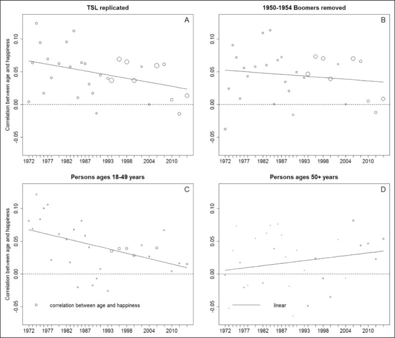
Trends in the correlation between age and happiness across years: scatterplots and linear regression lines. The 1982 and 1987 Black oversamples were removed, and the WTSSALL weight variable was used; circle size reflects relative sample size.

Second, the zero-order correlations used to measure the age–happiness relationship in these analyses are not appropriate, given that (and as TSL have also noted) the relationship between age and happiness is quadratic (this relationship generally has been found to increase from young adulthood to late middle age [ages 55–60] and then decline into older ages), and the correlation measures only linear association.³ In order to at least partially account for the quadratic nature of the age–happiness relationship, we separated the sample into two age groups: persons aged 18–49 years and persons aged 50+ years (50 years of age is the age at which TSL show that happiness begins to level off before it starts to decline around age 65).

Figure 3c and d shows that when the quadratic relationship between age and happiness is considered, the correlation between age and happiness declines among 18- to 49-year-olds across periods but increases for those aged 50 years and older. This finding significantly challenges TSL’s conclusion of a declining trend in mature adults’ happiness. Thus, as we have shown, the declining trend that TSL show in their Figure 3 is an artifact of two methodological shortcomings: (a) the inability to fully account for the well-known Baby Boomer cohort effect with such an approach and (b) the use of zero-order correlations to measure a quadratic relationship. In order to properly examine the age–happiness relationship, we must rely on more sophisticated methods that simultaneously examine the full extent of age, period, and cohort effects (e.g., see Yang & Land, 2006) while preserving the full sample size.

APC analyses of happiness

Disentangling age, period, and cohort effects is a difficult task, because these three dimensions of time are perfectly linearly related (i.e., cohort = period – age when the temporal widths of each of the three are identical; this identity does not necessarily hold for all observations in repeated cross-section sample survey research designs such as the GSS when the age at last birthday of each respondent is recorded and differential widths of the age, period, and cohort dimensions can be utilized; see Yang & Land, 2008) and therefore present an identification problem for statistical analyses that attempt to separate them. This identification problem is the central topic of a rich theoretical, methodological, and empirical literature that dates back to at least the 1960s (see Glenn, 1977/2005; Ryder, 1965; Schaie, 1965).

TSL used a recently developed APC method that breaks the linear dependency of the three dimensions of time via a hierarchical modeling strategy involving fixed and random effects.⁴ As used in TSL’s analyses, the age pattern in happiness is modeled as quadratic in shape, with the parameters for the linear and quadratic terms for age treated as fixed in Level 1 equation. The intercept in Level 1 equation is treated as random, with period and cohort patterns captured at Level 2. Thus,

$$\begin{gathered} \text{Level}1:y_{\mathit{ijk}}=b_{0jk}+b_1{\text{Age}}_{\mathit{ijk}}+b_2{\text{Age}}_{\mathit{ijk}}^2+e_{\mathit{ijk}}, \\ \text{Level}2:b_{0jk}=p_0+t_{0j}+c_{0k}. \end{gathered}$$

In this cross-classified random-effects HAPC model (Yang & Land, 2006), y_ijk is the ith person’s value of happiness in cohort j and period k, b_0jk is the intercept for happiness for cohort j in period k, b₁ is the linear effect of age for the ith person in cohort j and period k, b₂ is the quadratic effect of age for the ith person in cohort j and period k, e_ijk is an individual-cohort-period-specific error term assumed to follow the usual ordinary least squares (OLS) regression assumptions of homoscedasticity and independence, p₀ is a grand mean for happiness across all cohorts and time periods, t_0j is the residual random effect of period j on b_0jk—that is, the random effect of period j averaged over all cohorts, assumed normally distributed with mean 0, and c_0k is the residual random effect of cohort k on b_0jk—that is, the random effect of cohort k averaged over all periods.⁵

Using this method, we replicated TSL’s analyses of aggregated data, and we reanalyzed the data using single GSS waves for both the full adult sample (i.e., persons aged 18 plus) and age-group-specific samples (i.e., young adults and mature adults). Age is mean centered, in both the replicated and disaggregated analyses, at 44 years in the full sample models, at 24 years in the young adult models, and at 52 years in the mature adult models. Results are reported first for the full sample model and then for the age-group-specific models.⁶

Figure 4a and b, respectively, shows our replication of TSL’s cohort and period patterns in happiness. The cohort results show that the baby boomers are less happy than other cohorts, as evidenced by the “dip” in happiness for the four 5-year birth cohorts spanning from 1945 to 1964⁷ below the average level of happiness (net of age and period) represented by the horizontal line in Figure 4a. The replicated period results show that happiness has consistently decreased since about 2000. However, as we have already shown, aggregated period groupings can obscure potentially important period patterns in happiness. Thus, we reestimated TSL’s APC model using single-year GSS waves. Cohort patterns obtained from this model were consistent with TSL’s cohort results, but we found that the grouped 5-year period results missed at least two important features of the trend in happiness.

Figure 4.

(a) Cohort pattern in happiness net of age and period patterns: TSL’s age–period–cohort analysis (APC) model replicated. (b) Period pattern in happiness net of age and cohort patterns: TSL’s APC model replicated. (c) Period pattern in happiness net of age and cohort patterns: APC model with data disaggregated by single year.

First, TSL’s period pattern shows that happiness declines relatively consistently across time, with a sustained drop below the average happiness level after about 2000 (see Figure 4b). Yet, when GSS waves are disaggregated to show the full underlying pattern in the original data, the decline appears only to have begun during the Great Recession era (i.e., 2008–2010). Second, this decline appears to have been only temporary: There is a significant rebound in happiness after the Great Recession in the last two GSS waves. Indeed, by 2014, the confidence band shows that recent happiness levels are not statistically different from the long-term average across the entire observation period (1972–2014). This pattern sheds further light on how TSL’s aggregation of these data obscures important trends in the GSS data.

In order to examine the interaction between age and period, TSL conducted age-group-specific APC analyses. We replicated their period and cohort results and reanalyzed the age-group-specific period patterns using single waves of the GSS rather than TSL’s approximate 5-year groupings. The cohort patterns derived from our disaggregated analyses were consistent with TSL’s cohort patterns, but our other results yield two conclusions that differ substantially from those of TSL.

First, our reanalysis shows that there is no long-term decline in mature adults’ happiness nor a sustained increase in young adults’ happiness. Instead, we find that young and mature adults were affected by the Great Recession differently. On the one hand, young adults had a relatively rapid negative response followed by a relatively quick rebound, given that their happiness was statistically significantly lower than their long-term average only in 2008 (see Figure 5c). On the other hand, mature adults had a lagged negative response followed by a relatively slower rebound so that their happiness was significantly lower than their long-term average in the period from 2008 to 2012, but they returned to their long-term happiness level by 2014 (see Figure 5d).

Figure 5.

Cohort and period patterns in happiness for persons ages 18–29 years and 30 years and over.

Second, it is clear that TSL missed a key finding in their own analyses: Both pre- and post-boomer cohorts in fact became relatively happier as they aged from young to mature adults. Specifically, young adults’ happiness fluctuates around 2.15 units in Figure 5e, whereas non-boomer mature adults’ happiness fluctuates around 2.20 units (see Figure 5f). Therefore, the boomers are the only mature adults who are not aging as happily as mature adult members of other cohorts, and our finding confirms and extends that found in previous research (see Easterlin, 1980; Fukuda, 2013; Yang, 2008). Thus, the relationship between age and happiness has not disappeared in recent years but remains positive—just as TSL find in their APC analysis of the full adult age range but do not emphasize. Specifically, their initial APC analysis shows that, after controlling for cohort and period effects, the pattern in the relationship between age and happiness is quadratic! This finding completely undermines their conclusion.

Discussion

In this article, we have shown that TSL’s trend analyses (e.g., trend plots of mean happiness and trends in the bivariate correlations between age and happiness) are problematic for at least three reasons: (a) The authors, in their analysis of mean happiness trends, do not account for well-established cohort effects (i.e., lower happiness levels among baby boomers; see Fukuda, 2013), and these effects drive their results; (b) TSL, in this same trend analysis, (arbitrarily) aggregate GSS waves in a way that obscures age-group differences in the effects of the Great Recession on happiness, the true effects of which contradict their conclusions of a long-term decline in mature adults’ happiness; (c) The authors’ trend analysis of the bivariate correlation between age and happiness also does not account for the boomers, and it is fundamentally flawed because they use zero-order correlations to measure a quadratic relationship. Thus, as we have shown, this bivariate trend cannot fully account for the confounding nature of age, period, and cohort effects in happiness trends, and we must rely on more appropriate methods (e.g., Yang & Land, 2006).

TSL therefore use a more appropriate method in further analyses that enables removing the confounding influence of the boomers (i.e., HAPC methods; Yang & Land, 2006) to bolster their simpler analyses, but their aggregation of GSS data in these analyses is unwarranted and consequential. The consequence of aggregation is that what TSL show to be a consistent linear decline in mature adults’ happiness is, in fact, an artifact due to the differential effects of the Great Recession across age groups. Moreover, we find that the authors missed a key finding in their own mixed-effects regression analyses: Pre- and post-boomer cohorts are indeed happier as mature adults than boomers have been.

In sum, we found no evidence to support TSL’s conclusion that long-term cultural shifts have been favorable for young adults’ happiness relative to that of mature adults. To be fair, the authors noted that they could only speculate about their findings, and their interpretation appears to be guided by research that shows an increasing trend in individualism and unrealistic expectations for “educational attainment, jobs, material goods, and relationships” (e.g., Twenge & Campbell, 2008; Twenge & Kasser, 2013; p. 138). However, these apparent cultural shifts, in fact, seem to be unrelated to age trends in American adults’ happiness. Instead, the evidence that TSL show to support their conclusion simply reflects the aging of the Baby Boomers and the consequences of the Great Recession, coupled with their method of aggregation, and we are beginning to see a significant rebound to the established, long-term pattern as the Great Recession’s effects recede and the boomers age out of the population.

Biographies

Anthony R. Bardo is a National Institute on Aging postdoctoral scholar at Duke University. His research focuses on the intersections of health, well-being, and aging.

Scott M. Lynch is a professor of sociology and the director of an NIA-funded T32 training program on the Demography of Aging in the Duke University Population Research Institute at Duke University. His interests are in understanding socioeconomic, racial, and regional inequalities in health in the US across the life course and across birth cohorts, and in applied Bayesian statistical methods in demography and sociology.

Kenneth C. Land is the codirector of the Biodemography of Aging Research Unit (BARU) in the Center for Population Health and Aging, a unit of the Duke University Population Research Institute (DuPRI). His research interests and contributions are at the intersection of statistics, demography, criminology, and social indicators/quality-of-life/well-being studies.

References

- Bell DN, Blanchflower DG. Young people and the Great Recession. Oxford Review of Economic Policy. 2011;27:241–267. [Google Scholar]
- Bell A, Jones K. Should age-period-cohort analysts accept innovation without scrutiny? A response to Reither, Masters, Yang, Powers, Zheng, and Land. Social Science & Medicine. 2015;128:331–333. doi: 10.1016/j.socscimed.2015.01.040. [DOI] [PubMed] [Google Scholar]
- Blendon RJ, Benson JM. The public’s views about Medicare and the budget deficit. New England Journal of Medicine. 2011;365:e8. doi: 10.1056/NEJMp1107184. [DOI] [PubMed] [Google Scholar]
- Easterlin RA. Birth and fortune: The impact of numbers on personal welfare. Chicago, IL: University of Chicago; 1980. [Google Scholar]
- Fukuda K. A happiness study using age-period-cohort framework. Journal of Happiness Studies. 2013;14:135–153. [Google Scholar]
- Glenn ND. Cohort analysis. Thousand Oaks: Sage; 1977/2005. 1st & 2nd eds. [Google Scholar]
- Glenn ND. Is the apparent U-shape of well-being over the life course a result of inappropriate use of control variables? A commentary on Blanchflower and Oswald (66: 8, 2008, 1733–1749) Social Science & Medicine. 2009;69:481–485. doi: 10.1016/j.socscimed.2009.05.038. [DOI] [PubMed] [Google Scholar]
- Nauck B. Value of children and fertility: Results from a cross-cultural comparative survey in eighteen areas in Asia, Africa, Europe and America. Advances in Life Course Research. 2014;21:135–148. doi: 10.1016/j.alcr.2014.01.004. [DOI] [PubMed] [Google Scholar]
- Reither EN, Land KC, Jeon SY, Powers DA, Masters RK, Zheng H, Yang C. Clarifying hierarchical age-period-cohort models: A rejoinder to Bell and Jones. Social Science & Medicine. 2015;145:125–128. doi: 10.1016/j.socscimed.2015.07.013. [DOI] [PMC free article] [PubMed] [Google Scholar]
- Ryder NB. The cohort as a concept in the study of social change. American Sociological Review. 1965;30:843–861. [PubMed] [Google Scholar]
- Schaie KW. A general model for the study of developmental problems. Psychological Bulletin. 1965;64:92–107. doi: 10.1037/h0022371. [DOI] [PubMed] [Google Scholar]
- Twenge JM, Campbell WK. Increases in positive self-views among high school students: Birth cohort changes in anticipated performance, self-satisfaction, self-liking, and self-competence. Psychological Science. 2008;19:1082–1086. doi: 10.1111/j.1467-9280.2008.02204.x. [DOI] [PubMed] [Google Scholar]
- Twenge JM, Kasser T. Generational changes in materialism and work centrality, 1976–2007: Associations with temporal changes in societal insecurity and materialistic role-modeling. Personality and Social Psychology Bulletin. 2013;39:883–897. doi: 10.1177/0146167213484586. [DOI] [PubMed] [Google Scholar]
- Twenge JM, Sherman RA, Lyubomirsky S. More happiness for young people and less for mature adults: Time period differences in subjective well-being in the United States, 1972–2014. Social Psychological and Personality Science. 2016;7:131–141. [Google Scholar]
- Van Praag BMS, Ferrer-i-Carbonell A. Happiness quantified: A satisfaction calculus approach. Oxford: Oxford University Press; 2008. [Google Scholar]
- Yang Y. Social inequalities in happiness in the United States, 1972–2004: An age-period-cohort analysis. American Sociological Review. 2008;73:204–226. [Google Scholar]
- Yang Y, Land KC. A mixed models approach to the age-period-cohort analysis of repeated cross-section surveys, with an application to data on trends in verbal test scores. Sociological Methodology. 2006;36:75–97. [Google Scholar]
- Yang Y, Land KC. Age-period-cohort analysis of repeated cross-section surveys: Fixed or random effects? Sociological Methods & Research. 2008;36:297–326. [Google Scholar]